CSE574 - Administriva No class on Fri 01/25 (Ski Day) TexPoint fonts used in EMF. Read the TexPoint...
54
CSE574 - Administriva • No class on Fri 01/25 (Ski Day)
-
date post
20-Dec-2015 -
Category
Documents
-
view
213 -
download
0
Transcript of CSE574 - Administriva No class on Fri 01/25 (Ski Day) TexPoint fonts used in EMF. Read the TexPoint...

CSE574 - Administriva• No class on Fri 01/25 (Ski Day)
Last Wednesday• HMMs
– Most likely individual state at time t: (forward)– Most likely sequence of states (Viterbi)– Learning using EM
• Generative vs. Discriminative Learning– Model p(y,x) vs. p(y|x)– p(y|x) : don’t bother about p(x) if we only want
to do classification
Today• Markov Networks
– Most likely individual state at time t: (forward)
– Most likely sequence of states (Viterbi)– Learning using EM
• CRFs– Model p(y,x) vs. p(y|x)– p(y|x) : don’t bother about p(x) if we only
want to do classification

Finite State Models
Naïve Bayes
Logistic Regression
Linear-chain CRFs
HMMsGenerative
directed models
General CRFs
Sequence
Sequence
Conditional Conditional Conditional
GeneralGraphs
GeneralGraphs
Figure by Sutton & McCallum
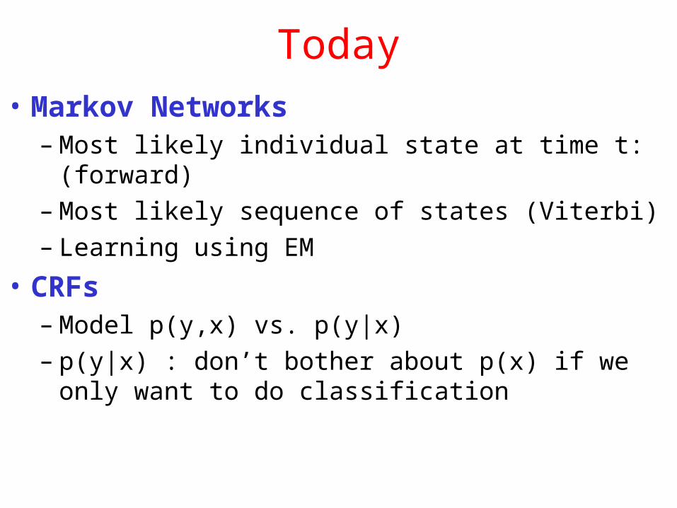
Graphical Models• Family of probability distributions that factorize
in a certain way• Directed (Bayes Nets)
• Undirected (Markov Random Field)
• Factor Graphs
x0
x1x2
x3
x4
p(x) =Q K
i=1 p(xi jP arents(xi))
p(x) = 1Z
QA ª A (xA )
x = x1x2 : : :xK
x0
x1x2
x4
x3x5
ª A factor function
A ½fx1; : : :;xK g
x0
x1x2
x4
x3x5
p(x) = 1Z
QC ª C (xC )
C ½fx1; : : :;xK g clique
ª C potential function
Node is independent of its non-descendants given its
parentsNode is independent all other
nodes given its neighbors

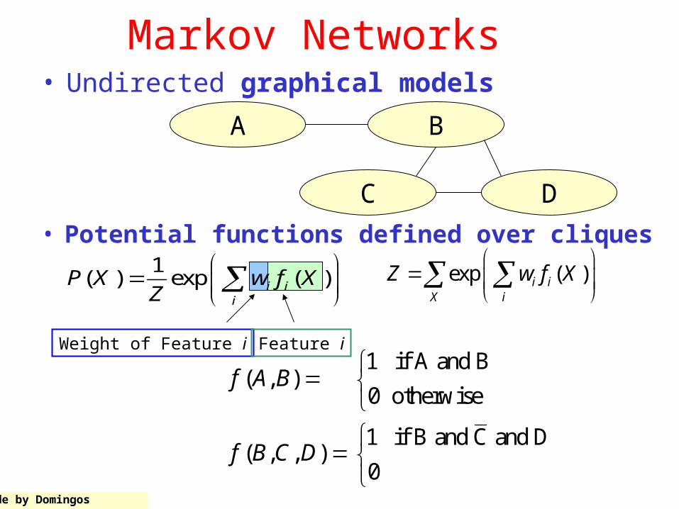
Markov Networks• Undirected graphical models
B
DC
A
1( ) ( )c
c
P X XZ
3.7 if A and B
( , ) 2.1 if A and B
0.7 otherwise
2.3 if B and C and D( , , )
5.1 otherwise
A B
B C D
( )cX c
Z X • Potential functions defined over cliques
Slide by Domingos
Markov Networks• Undirected graphical models
B
DC
A
• Potential functions defined over cliques
Weight of Feature i Feature i
exp ( )i iX i
Z w f X
1( ) exp ( )i i
i
P X w f XZ
1 if A and B ( , )
0 otherwise
1 if B and C and D( , , )
0
f A B
f B C D
Slide by Domingos

Hammersley-Clifford Theorem
If Distribution is strictly positive (P(x) > 0)
And Graph encodes conditional independences
Then Distribution is product of potentials over cliques of graph
Inverse is also true.
Slide by Domingos
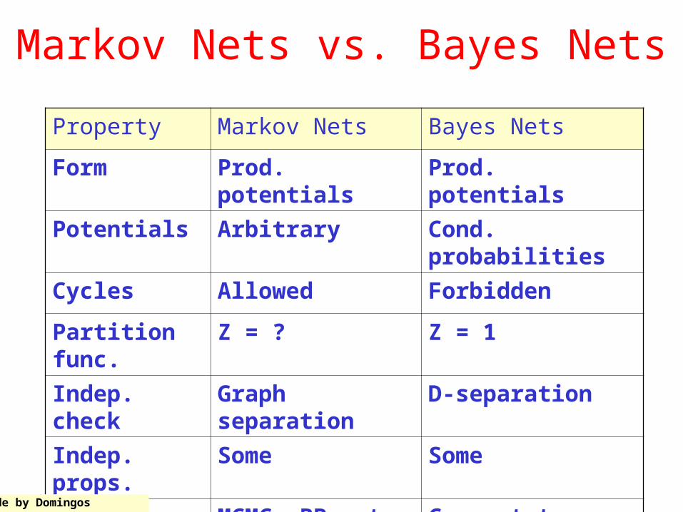
Markov Nets vs. Bayes Nets
Property Markov Nets Bayes Nets
Form Prod. potentials
Prod. potentials
Potentials Arbitrary Cond. probabilities
Cycles Allowed Forbidden
Partition func.
Z = ? Z = 1
Indep. check
Graph separation
D-separation
Indep. props.
Some Some
Inference MCMC, BP, etc. Convert to Markov
Slide by Domingos

Inference in Markov Networks• Goal: compute marginals & conditionals
of
• Exact inference is #P-complete• Conditioning on Markov blanket is easy:
• Gibbs sampling exploits this
exp ( )( | ( ))
exp ( 0) exp ( 1)
i ii
i i i ii i
w f xP x MB x
w f x w f x
1( ) exp ( )i i
i
P X w f XZ
exp ( )i i
X i
Z w f X
Slide by Domingos
E.g.: What is ?What is ?P (xi jx1; : : :;xi ¡ 1;xi+1; : : :;xN )
P (xi )

Markov Chain Monte Carlo• Idea:
– create chain of samples x(1), x(2), …where x(i+1) depends on x(i)
– set of samples x(1), x(2), … used to approximate p(x)
X 1
X 2
X 3
X 4 X 5
x(1) = (X 1 = x(1)1 ;X 2 = x(1)
2 ; : : :;X5 = x(1)5 )
x(2) = (X 1 = x(2)1 ;X 2 = x(2)
2 ; : : :;X5 = x(2)5 )
x(3) = (X 1 = x(3)1 ;X 2 = x(3)
2 ; : : :;X5 = x(3)5 )
Slide by Domingos
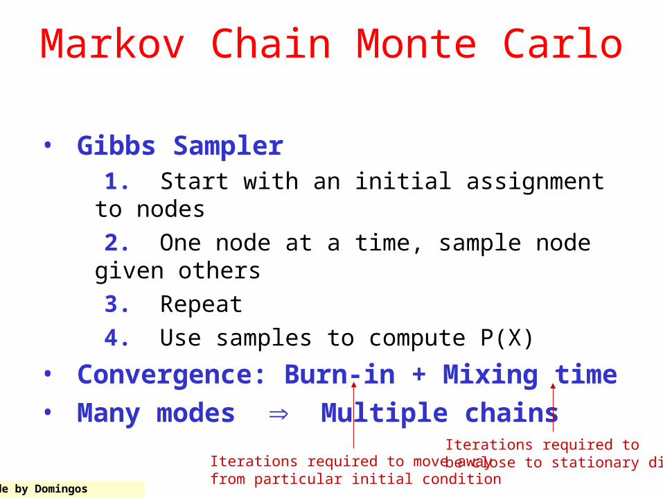
Markov Chain Monte Carlo
• Gibbs Sampler 1. Start with an initial assignment to nodes 2. One node at a time, sample node given
others 3. Repeat 4. Use samples to compute P(X)
• Convergence: Burn-in + Mixing time
• Many modes Multiple chainsIterations required to move away from particular initial condition
Iterations required tobe close to stationary dist.
Slide by Domingos

Other Inference Methods• Belief propagation (sum-product)• Mean field / Variational
approximations
Slide by Domingos
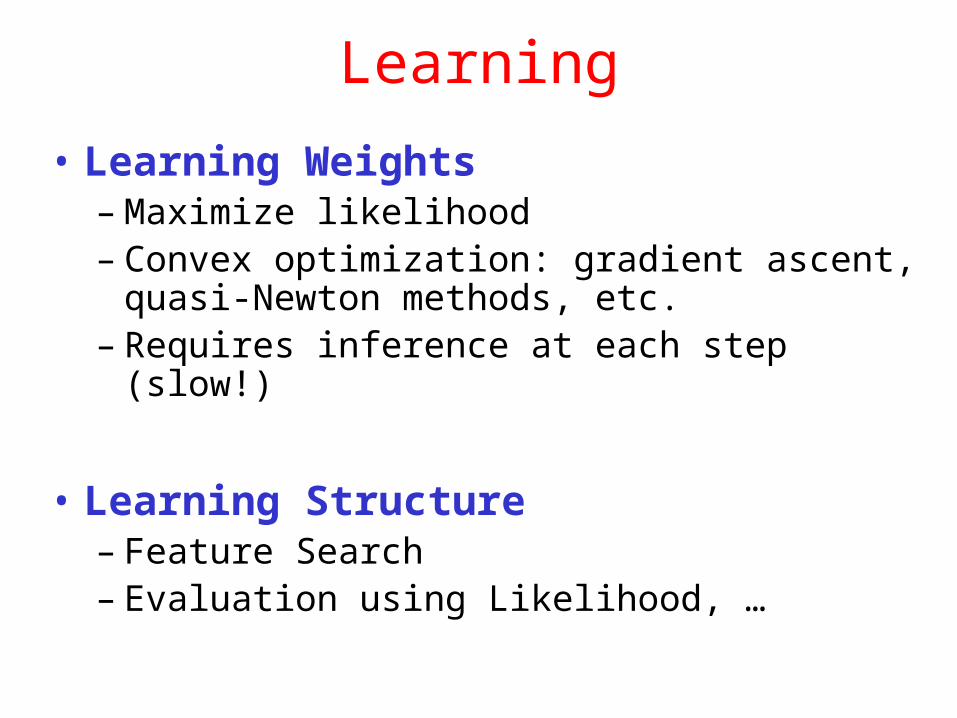
Learning
• Learning Weights– Maximize likelihood– Convex optimization: gradient ascent,
quasi-Newton methods, etc.– Requires inference at each step (slow!)
• Learning Structure– Feature Search– Evaluation using Likelihood, …

Back to CRFs• CRFs are conditionally trained
Markov Networks

Linear-Chain Conditional Random Fields
• From HMMs to CRFs
can also be written as
(set , …)We let new parameters vary freely, so
weneed normalization constant Z.
p(y;x) =TY
t=1
p(yt jyt¡ 1)p(xtjyt)
p(y;x) =1Z
exp
0
@X
t
X
i ;j 2S
¸ i j 1f yt =ig1f yt ¡ 1=j g +X
t
X
i 2S
X
o2O
¹ oi 1f yt =ig1f xt =og
1
A
¸ i j := logp(y0= ijy = j )
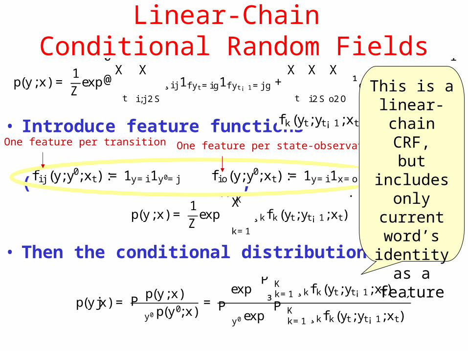
Linear-Chain Conditional Random Fields
• Introduce feature functions
( , )
• Then the conditional distribution is
f k(yt;yt¡ 1;xt)
f i j (y;y0;xt) := 1y=i 1y0=j
p(y;x) =1Z
exp
0
@X
t
X
i ;j 2S
¸ i j 1f yt =ig1f yt ¡ 1=j g +X
t
X
i 2S
X
o2O
¹ oi 1f yt =ig1f xt =og
1
A
p(y;x) =1Z
exp
ÃKX
k=1
¸kf k(yt;yt¡ 1;xt)
!
p(yjx) =p(y;x)
Py0 p(y0;x)
=exp
³ P Kk=1 ¸kf k(yt ;yt¡ 1;xt)
´
Py0 exp
³ P Kk=1 ¸kf k(yt ;yt¡ 1;xt)
´
f i o(y;y0;xt) := 1y=i 1x=o
One feature per transition One feature per state-observation pair
This is a linear-
chain CRF,but
includes only
current word’s
identity as a feature

Linear-Chain Conditional Random Fields
• Conditional p(y|x) that follows from joint p(y,x) of HMM is a linear CRF with certain feature functions!

p(yjx) =1
Z(x)exp
ÃKX
k=1
¸k f k(yt ;yt¡ 1;xt)
!
Linear-Chain Conditional Random Fields
• Definition:A linear-chain CRF is a distribution that takes the form
where Z(x) is a normalization function
Z(x) =X
y
exp
ÃKX
k=1
¸kf k(yt;yt¡ 1;xt)
!
parameters
feature functions
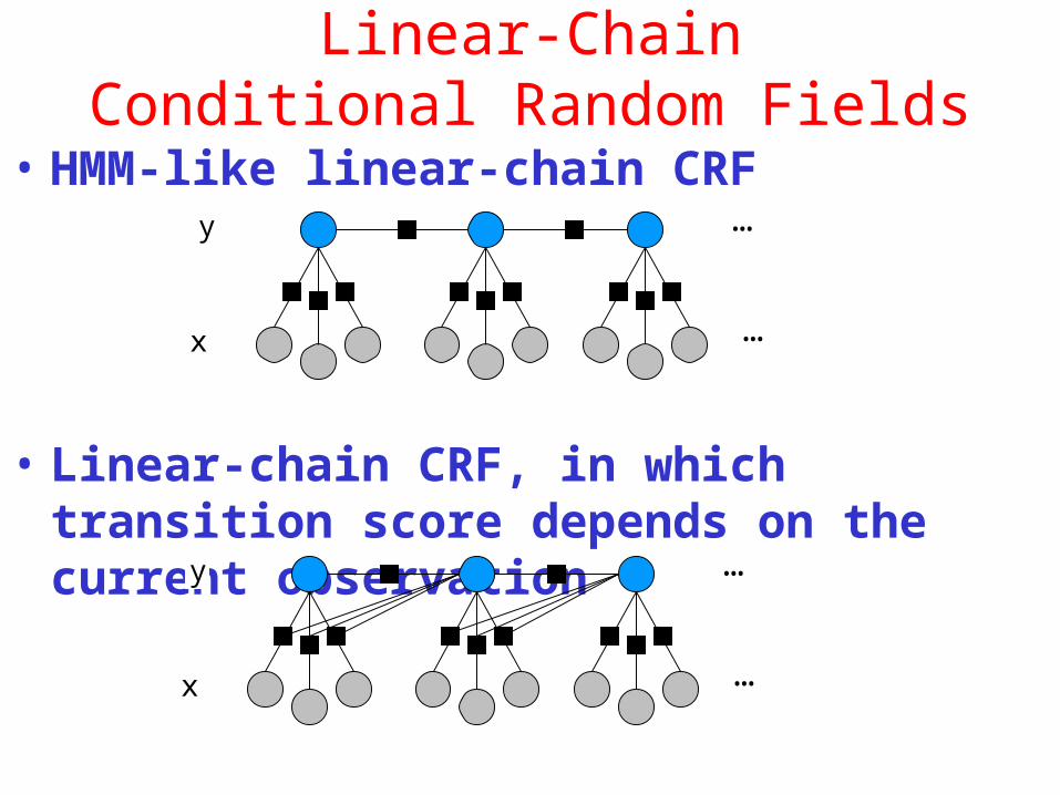
Linear-ChainConditional Random Fields
• HMM-like linear-chain CRF
• Linear-chain CRF, in which transition score depends on the current observation
…
…x
y
…
…x
y
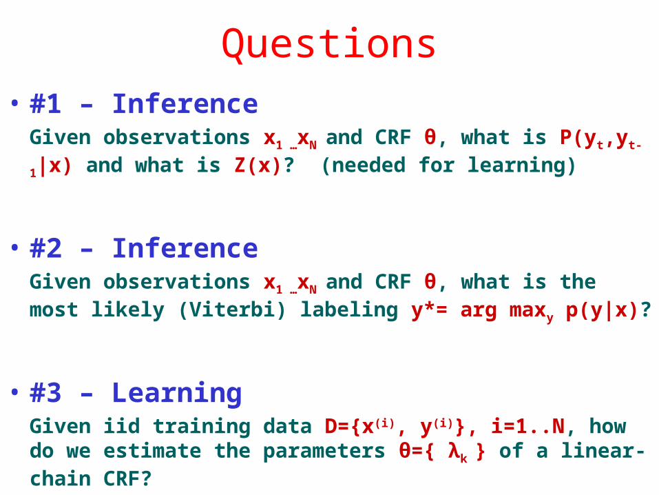
Questions• #1 – Inference
Given observations x1 …xN and CRF θ, what is P(yt,yt-
1|x) and what is Z(x)? (needed for learning)
• #2 – InferenceGiven observations x1 …xN and CRF θ, what is the most likely (Viterbi) labeling y*= arg maxy p(y|x)?
• #3 – LearningGiven iid training data D={x(i), y(i)}, i=1..N, how do we estimate the parameters θ={ λk } of a linear-chain CRF?
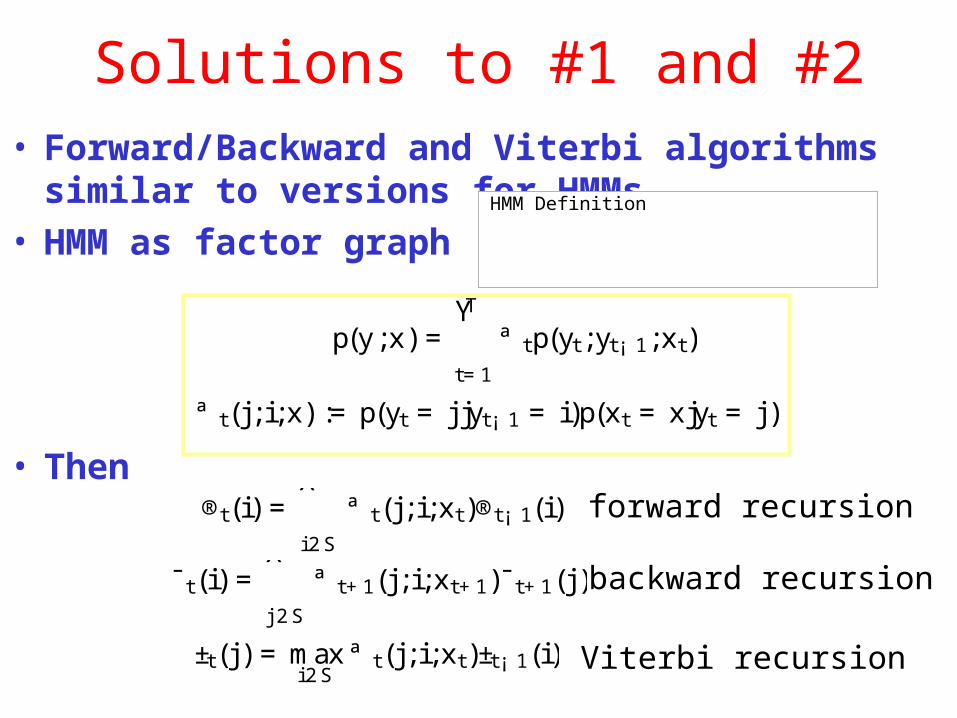
Solutions to #1 and #2• Forward/Backward and Viterbi algorithms
similar to versions for HMMs• HMM as factor graph
• Then
p(y;x) =TY
t=1
p(yt jyt¡ 1)p(xtjyt)
p(y;x) =TY
t=1
ª tp(yt;yt¡ 1;xt)
ª t(j ; i;x) := p(yt = j jyt¡ 1 = i)p(xt = xjyt = j )
¯t(i) =X
j 2S
ª t+1(j ; i;xt+1)¯t+1(j )
®t(i) =X
i 2S
ª t(j ; i;xt)®t¡ 1(i)
±t(j ) = maxi2S
ª t(j ; i;xt)±t¡ 1(i)
forward recursion
backward recursion
Viterbi recursion
HMM Definition
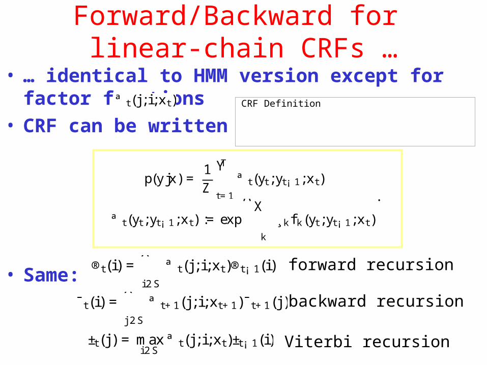
Forward/Backward for linear-chain CRFs …
• … identical to HMM version except for factor functions
• CRF can be written as
• Same:
p(yjx) =1Z
TY
t=1
ª t(yt;yt¡ 1;xt)
ª t(yt;yt¡ 1;xt) := exp
ÃX
k
¸kf k(yt;yt¡ 1;xt)
!
ª t(j ; i;xt)
¯t(i) =X
j 2S
ª t+1(j ; i;xt+1)¯t+1(j )
®t(i) =X
i 2S
ª t(j ; i;xt)®t¡ 1(i)
±t(j ) = maxi2S
ª t(j ; i;xt)±t¡ 1(i)
forward recursion
backward recursion
Viterbi recursion
p(yjx) =1Z
exp
ÃKX
k=1
¸kf k(yt;yt¡ 1;xt)
! CRF Definition
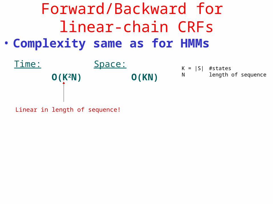
Forward/Backward for linear-chain CRFs
• Complexity same as for HMMs
Time:O(K2N)
Space:O(KN)
K = |S| #statesN length of sequence
Linear in length of sequence!
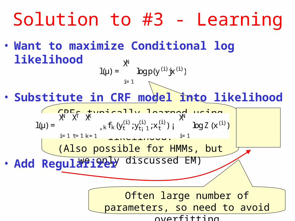
Solution to #3 - Learning• Want to maximize Conditional log
likelihoodl(µ) =
NX
i=1
logp(y(i ) jx(i ))
CRFs typically learned using numerical optimization of
likelihood.(Also possible for HMMs, but we
only discussed EM)
¡KX
k=1
¸2k
2¾2
Often large number of parameters, so need to avoid overfitting
• Add Regularizer
l(µ) =NX
i=1
TX
t=1
KX
k=1
¸kf k(y(i )t ;y(i )
t¡ 1;x(i )t ) ¡
NX
i=1
logZ(x(i ))
• Substitute in CRF model into likelihood

Regularization• Commonly used l2-norm (Euclidean)
– Corresponds to Gaussian prior over parameters
• Alternative is l1-norm– Corresponds to exponential prior over parameters– Encourages sparsity
• Accuracy of final model not sensitive to
¡KX
k=1
¸2k
2¾2
¡KX
k=1
j¸kj¾
¾

Optimizing the Likelihood• There exists no closed-form solution, so must
use numerical optimization.
l(µ) =NX
i=1
TX
t=1
KX
k=1
¸kf k(y(i )t ;y(i )
t¡ 1;x(i )t ) ¡
NX
i=1
logZ(x(i )) ¡KX
k=1
¸2k
2¾2
@l@̧ k
=NX
i=1
TX
t=1
f k(y(i )t ;y(i )
t¡ 1;x(i )t ) ¡
NX
i=1
TX
t=1
X
y;y0
f k(y;y0;x(i )t )p(y;y0jx(i )) ¡
KX
k=1
¸k
¾2
Figure by Cohen & McCallum
• l(θ) is concave and with regularizer strictly concave
only one global optimum

Optimizing the Likelihood• Steepest Ascent
very slow!
• Newton’s methodfewer iterations, but requires Hessian-1
• Quasi-Newton methodsapproximate Hessian by analyzing successive gradients
– BFGSfast, but approximate Hessian requires quadratic
space
– L-BFGS (limited-memory)fast even with limited memory!
– Conjugate Gradient

Computational Cost
l(µ) =NX
i=1
TX
t=1
KX
k=1
¸kf k(y(i )t ;y(i )
t¡ 1;x(i )t ) ¡
NX
i=1
logZ(x(i )) ¡KX
k=1
¸2k
2¾2
@l@̧ k
=NX
i=1
TX
t=1
f k(y(i )t ;y(i )
t¡ 1;x(i )t ) ¡
NX
i=1
TX
t=1
X
y;y0
f k(y;y0;x(i )t )p(y;y0jx(i )) ¡
KX
k=1
¸k
¾2
• For each training instance: O(K2T) (using forward-backward)
• For N training instances, G iterations: O(K2TNG)
Examples:- Named-entity recognition 11 labels; 200,000 words < 2 hours- Part-of-speech tagging 45 labels, 1 million words > 1 week

Person name Extraction[McCallum 2001, unpublished]
Slide by Cohen & McCallum

Person name Extraction
Slide by Cohen & McCallum
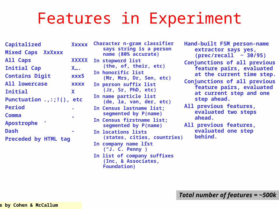
Features in Experiment
Capitalized XxxxxMixed Caps XxXxxxAll Caps
XXXXXInitial Cap X….Contains Digit xxx5All lowercase xxxxInitial XPunctuation .,:;!(), etcPeriod .Comma ,Apostrophe ‘Dash -Preceded by HTML tag
Character n-gram classifier says string is a person name (80% accurate)
In stopword list(the, of, their, etc)
In honorific list(Mr, Mrs, Dr, Sen, etc)
In person suffix list(Jr, Sr, PhD, etc)
In name particle list (de, la, van, der, etc)
In Census lastname list;segmented by P(name)
In Census firstname list;segmented by P(name)
In locations lists(states, cities, countries)
In company name list(“J. C. Penny”)
In list of company suffixes(Inc, & Associates, Foundation)
Hand-built FSM person-name extractor says yes, (prec/recall ~ 30/95)
Conjunctions of all previous feature pairs, evaluated at the current time step.
Conjunctions of all previous feature pairs, evaluated at current step and one step ahead.
All previous features, evaluated two steps ahead.
All previous features, evaluated one step behind.
Total number of features = ~500k
Slide by Cohen & McCallum

Training and Testing• Trained on 65k words from 85 pages, 30
different companies’ web sites.• Training takes 4 hours on a 1 GHz Pentium.• Training precision/recall is 96% / 96%.
• Tested on different set of web pages with similar size characteristics.
• Testing precision is 92 – 95%, recall is 89 – 91%.
Slide by Cohen & McCallum

Part-of-speech Tagging
The asbestos fiber , crocidolite, is unusually resilient once
it enters the lungs , with even brief exposures to it causing
symptoms that show up decades later , researchers said .
DT NN NN , NN , VBZ RB JJ IN
PRP VBZ DT NNS , IN RB JJ NNS TO PRP VBG
NNS WDT VBP RP NNS JJ , NNS VBD .
45 tags, 1M words training data, Penn Treebank
Error oov error error err oov error err
HMM 5.69% 45.99%
CRF 5.55% 48.05% 4.27% -24% 23.76% -50%
Using spelling features*
* use words, plus overlapping features: capitalized, begins with #, contains hyphen, ends in -ing, -ogy, -ed, -s, -ly, -ion, -tion, -ity, -ies.
[Lafferty, McCallum, Pereira 2001] Slide by Cohen & McCallum
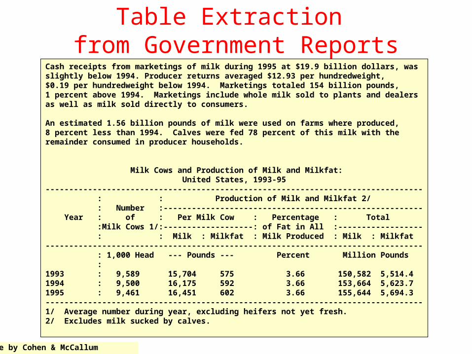
Table Extraction from Government Reports
Cash receipts from marketings of milk during 1995 at $19.9 billion dollars, was slightly below 1994. Producer returns averaged $12.93 per hundredweight, $0.19 per hundredweight below 1994. Marketings totaled 154 billion pounds, 1 percent above 1994. Marketings include whole milk sold to plants and dealers as well as milk sold directly to consumers. An estimated 1.56 billion pounds of milk were used on farms where produced, 8 percent less than 1994. Calves were fed 78 percent of this milk with the remainder consumed in producer households. Milk Cows and Production of Milk and Milkfat: United States, 1993-95 -------------------------------------------------------------------------------- : : Production of Milk and Milkfat 2/ : Number :------------------------------------------------------- Year : of : Per Milk Cow : Percentage : Total :Milk Cows 1/:-------------------: of Fat in All :------------------ : : Milk : Milkfat : Milk Produced : Milk : Milkfat -------------------------------------------------------------------------------- : 1,000 Head --- Pounds --- Percent Million Pounds : 1993 : 9,589 15,704 575 3.66 150,582 5,514.4 1994 : 9,500 16,175 592 3.66 153,664 5,623.7 1995 : 9,461 16,451 602 3.66 155,644 5,694.3 --------------------------------------------------------------------------------1/ Average number during year, excluding heifers not yet fresh. 2/ Excludes milk sucked by calves.
Slide by Cohen & McCallum

Table Extraction from Government Reports
Cash receipts from marketings of milk during 1995 at $19.9 billion dollars, was
slightly below 1994. Producer returns averaged $12.93 per hundredweight,
$0.19 per hundredweight below 1994. Marketings totaled 154 billion pounds,
1 percent above 1994. Marketings include whole milk sold to plants and dealers
as well as milk sold directly to consumers.
An estimated 1.56 billion pounds of milk were used on farms where produced,
8 percent less than 1994. Calves were fed 78 percent of this milk with the
remainder consumed in producer households.
Milk Cows and Production of Milk and Milkfat:
United States, 1993-95
--------------------------------------------------------------------------------
: : Production of Milk and Milkfat 2/
: Number :-------------------------------------------------------
Year : of : Per Milk Cow : Percentage : Total
:Milk Cows 1/:-------------------: of Fat in All :------------------
: : Milk : Milkfat : Milk Produced : Milk : Milkfat
--------------------------------------------------------------------------------
: 1,000 Head --- Pounds --- Percent Million Pounds
:
1993 : 9,589 15,704 575 3.66 150,582 5,514.4
1994 : 9,500 16,175 592 3.66 153,664 5,623.7
1995 : 9,461 16,451 602 3.66 155,644 5,694.3
--------------------------------------------------------------------------------
1/ Average number during year, excluding heifers not yet fresh.
2/ Excludes milk sucked by calves.
CRFLabels:• Non-Table• Table Title• Table Header• Table Data Row• Table Section Data Row• Table Footnote• ... (12 in all)
[Pinto, McCallum, Wei, Croft, 2003]
Features:• Percentage of digit chars• Percentage of alpha chars• Indented• Contains 5+ consecutive spaces• Whitespace in this line aligns with
prev.• ...• Conjunctions of all previous features,
time offset: {0,0}, {-1,0}, {0,1}, {1,2}.
100+ documents from www.fedstats.gov
Slide by Cohen & McCallum
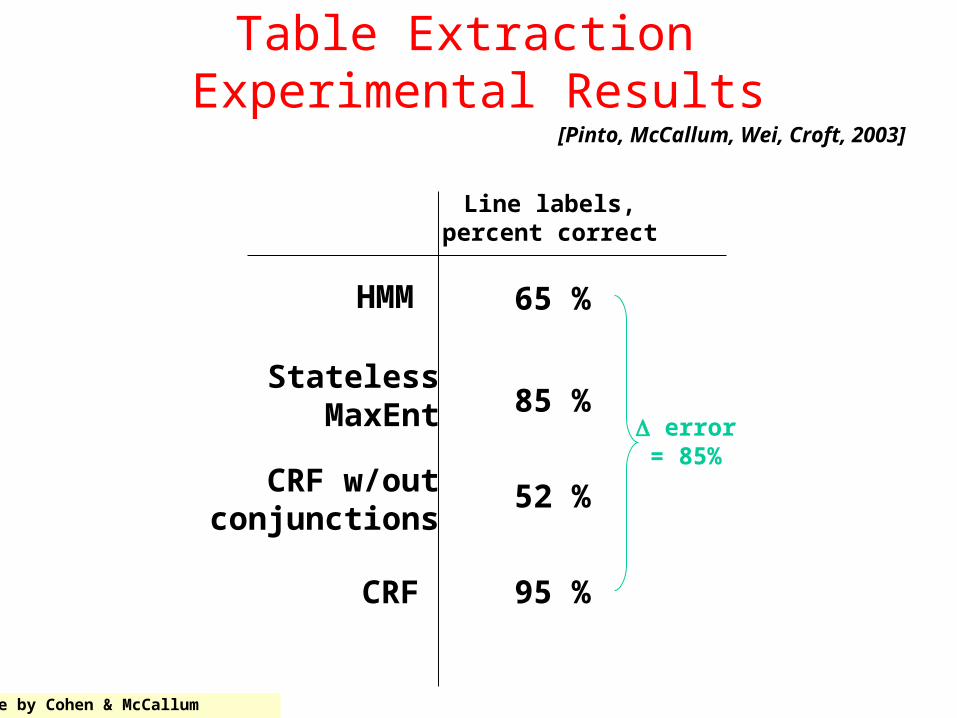
Table Extraction Experimental Results
Line labels,percent correct
95 %
65 %
error = 85%
85 %
HMM
StatelessMaxEnt
CRF w/outconjunctions
CRF
52 %
[Pinto, McCallum, Wei, Croft, 2003]
Slide by Cohen & McCallum

Named Entity Recognition
CRICKET - MILLNS SIGNS FOR BOLAND
CAPE TOWN 1996-08-22
South African provincial side Boland said on Thursday they had signed Leicestershire fast bowler David Millns on a one year contract. Millns, who toured Australia with England A in 1992, replaces former England all-rounder Phillip DeFreitas as Boland's overseas professional.
Labels: Examples:
PER Yayuk BasukiInnocent Butare
ORG 3MKDPLeicestershire
LOC LeicestershireNirmal HridayThe Oval
MISC JavaBasque1,000 Lakes Rally
Reuters stories on international news Train on ~300k words
Slide by Cohen & McCallum

Automatically Induced Features
Index Feature
0 inside-noun-phrase (ot-1)
5 stopword (ot)
20 capitalized (ot+1)
75 word=the (ot)
100 in-person-lexicon (ot-1)
200 word=in (ot+2)
500 word=Republic (ot+1)
711 word=RBI (ot) & header=BASEBALL
1027 header=CRICKET (ot) & in-English-county-lexicon (ot)
1298 company-suffix-word (firstmentiont+2)
4040 location (ot) & POS=NNP (ot) & capitalized (ot) & stopword (ot-1)
4945 moderately-rare-first-name (ot-1) & very-common-last-name (ot)
4474 word=the (ot-2) & word=of (ot)
[McCallum 2003]
Slide by Cohen & McCallum
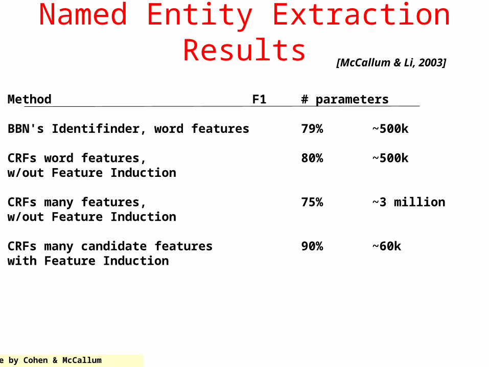
Named Entity Extraction Results
Method F1 # parameters
BBN's Identifinder, word features 79% ~500k
CRFs word features, 80% ~500kw/out Feature Induction
CRFs many features, 75% ~3 millionw/out Feature Induction
CRFs many candidate features 90% ~60kwith Feature Induction
[McCallum & Li, 2003]
Slide by Cohen & McCallum

So far …• … only looked at linear-chain CRFs
p(yjx) =1
Z(x)exp
ÃKX
k=1
¸k f k(yt ;yt¡ 1;xt)
!
parameters
feature functions
…
…x
y
…
…x
y
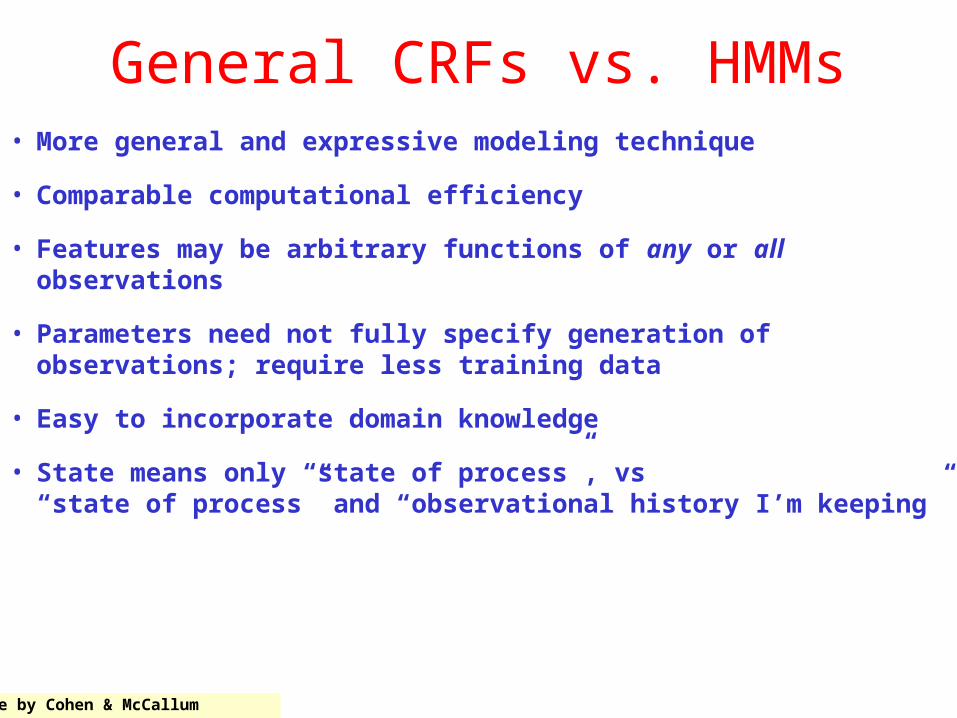
General CRFs vs. HMMs• More general and expressive modeling technique
• Comparable computational efficiency
• Features may be arbitrary functions of any or all observations
• Parameters need not fully specify generation of observations; require less training data
• Easy to incorporate domain knowledge
• State means only “state of process”, vs“state of process” and “observational history I’m keeping”
Slide by Cohen & McCallum
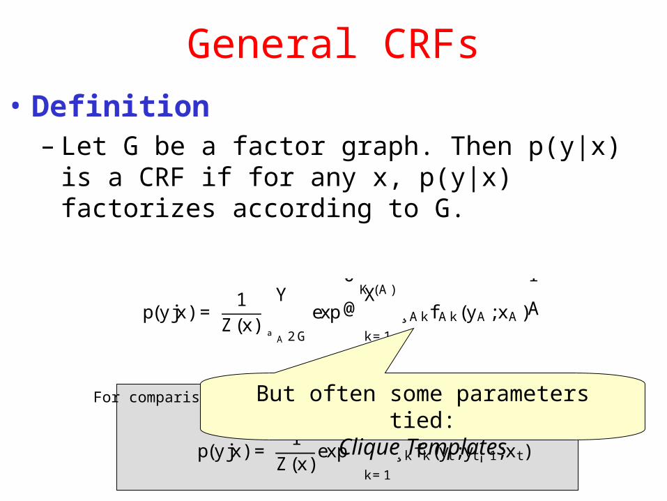
General CRFs• Definition
– Let G be a factor graph. Then p(y|x) is a CRF if for any x, p(y|x) factorizes according to G.
p(yjx) =1
Z(x)
Y
ª A 2G
exp
0
@K (A )X
k=1
¸A kfA k(yA ;xA )
1
A
p(yjx) =1
Z(x)exp
ÃKX
k=1
¸k f k(yt ;yt¡ 1;xt)
!For comparison: linear-chain CRFsBut often some parameters tied:
Clique Templates
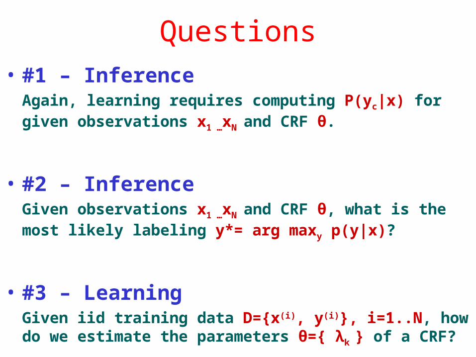
Questions• #1 – Inference
Again, learning requires computing P(yc|x) for given observations x1 …xN and CRF θ.
• #2 – InferenceGiven observations x1 …xN and CRF θ, what is the most likely labeling y*= arg maxy p(y|x)?
• #3 – LearningGiven iid training data D={x(i), y(i)}, i=1..N, how do we estimate the parameters θ={ λk } of a CRF?
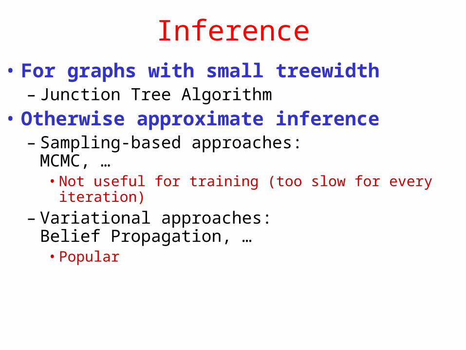
Inference• For graphs with small treewidth
– Junction Tree Algorithm• Otherwise approximate inference
– Sampling-based approaches: MCMC, …• Not useful for training (too slow for every iteration)
– Variational approaches:Belief Propagation, …• Popular

Learning• Similar to linear-chain case• Substitute model into likelihood …
… and compute partial derivatives, …
and run nonlinear optimization (L-BFGS)
l(µ) =X
Cp2C
X
ª c 2Cp
K (p)X
k=1
¸pkfpk(xx;yc) ¡ logZ(x)
@l@̧ pk
=X
ª c 2Cp
fpk(xc;yc) ¡X
ª c 2Cp
X
y0c
fpk(xc;y0c)p(y0
cjx)
inference
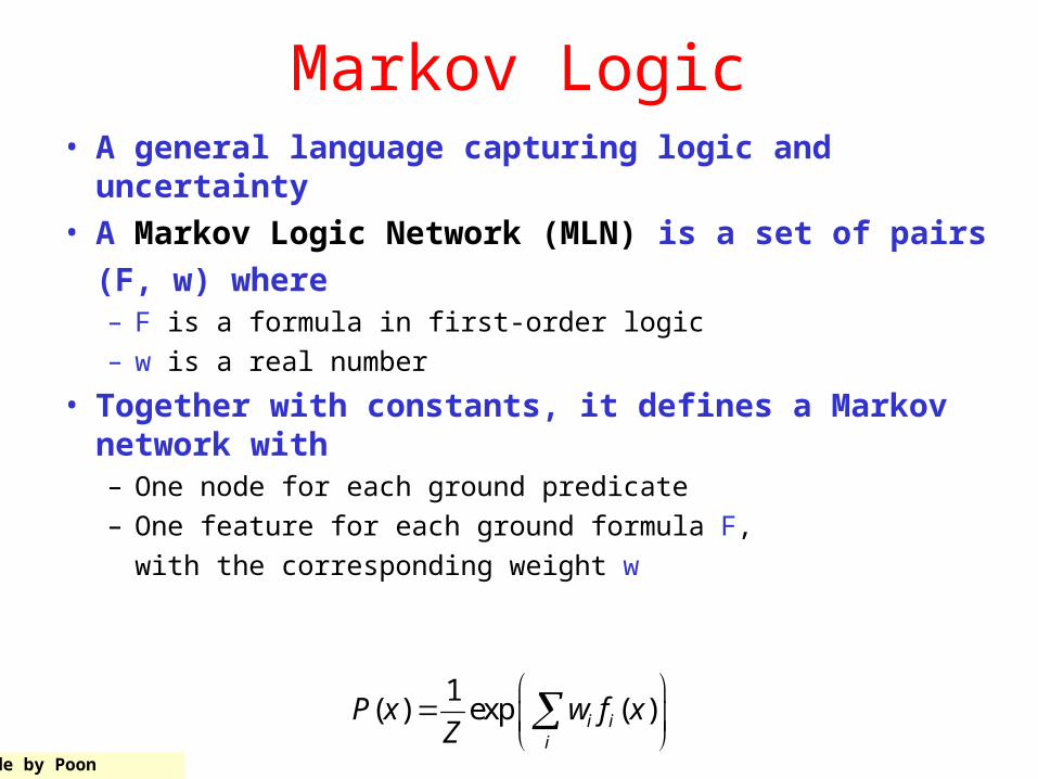
Markov Logic• A general language capturing logic and
uncertainty• A Markov Logic Network (MLN) is a set of pairs
(F, w) where– F is a formula in first-order logic– w is a real number
• Together with constants, it defines a Markov network with– One node for each ground predicate– One feature for each ground formula F,
with the corresponding weight w
1( ) exp ( )i i
i
P x w f xZ
Slide by Poon

Example of an MLN
)()(),(,
)()(
ySmokesxSmokesyxFriendsyx
xCancerxSmokesx
1.1
5.1
Cancer(A)
Smokes(A) Smokes(B)
Cancer(B)
Suppose we have two constants: Anna (A) and Bob (B)
Slide by Domingos

Example of an MLN
)()(),(,
)()(
ySmokesxSmokesyxFriendsyx
xCancerxSmokesx
1.1
5.1
Cancer(A)
Smokes(A)Friends(A,A)
Friends(B,A)
Smokes(B)
Friends(A,B)
Cancer(B)
Friends(B,B)
Suppose we have two constants: Anna (A) and Bob (B)
Slide by Domingos

Example of an MLN
)()(),(,
)()(
ySmokesxSmokesyxFriendsyx
xCancerxSmokesx
1.1
5.1
Cancer(A)
Smokes(A)Friends(A,A)
Friends(B,A)
Smokes(B)
Friends(A,B)
Cancer(B)
Friends(B,B)
Suppose we have two constants: Anna (A) and Bob (B)
Slide by Domingos

Example of an MLN
)()(),(,
)()(
ySmokesxSmokesyxFriendsyx
xCancerxSmokesx
1.1
5.1
Cancer(A)
Smokes(A)Friends(A,A)
Friends(B,A)
Smokes(B)
Friends(A,B)
Cancer(B)
Friends(B,B)
Suppose we have two constants: Anna (A) and Bob (B)
Slide by Domingos

Joint Inference in Information Extraction
Hoifung PoonDept. Computer Science & Eng.
University of Washington
(Joint work with Pedro Domingos)
Slide by Poon

Problems of Pipeline Inference
• AI systems typically use pipeline architecture– Inference is carried out in stages– E.g., information extraction, natural language
processing, speech recognition, vision, robotics
• Easy to assemble & low computational cost, but …– Errors accumulate along the pipeline– No feedback from later stages to earlier ones
• Worse: Often process one object at a time
Slide by Poon

We Need Joint Inference
?
S. Minton Integrating heuristics for constraint satisfaction problems: A case study. In AAAI Proceedings, 1993.
Minton, S(1993 b). Integrating heuristics for constraint satisfaction problems: A case study. In: Proceedings AAAI.
Author Title
Slide by Poon