CRISTHIANE ASSENHAIMER - USP€¦ · 5.8.2. Neural Network Fitting for Evaluating Status...
131
CRISTHIANE ASSENHAIMER Evaluation of Emulsion Destabilization by Light Scattering Applied to Metalworking Fluids Tese apresentada à Escola Politécnica da Universidade de São Paulo para obtenção do título de Doutor em Engenharia São Paulo 2015
Transcript of CRISTHIANE ASSENHAIMER - USP€¦ · 5.8.2. Neural Network Fitting for Evaluating Status...

CRISTHIANE ASSENHAIMER
Evaluation of Emulsion Destabilization by Light Scattering Applied to Metalworking Fluids
Tese apresentada à Escola Politécnica da Universidade de São Paulo para obtenção do título de Doutor em Engenharia
São Paulo 2015

CRISTHIANE ASSENHAIMER
Evaluation of Emulsion Destabilization by Light Scattering Applied to Metalworking Fluids
Tese apresentada à Escola Politécnica da Universidade de São Paulo para obtenção do título de Doutor em Engenharia Área de concentração: Engenharia Química Orientador: Prof. Dr. Roberto Guardani
São Paulo 2015

Este exemplar foi revisado e corrigido em relação à versão original, sob responsabilidade única do autor e com a anuência de seu orientador.
São Paulo, fil_ de~ de J.Q l s Assinatura do autor:
Assinatura do orientador:
Catalogação-na-publicação
Assenhaimer, Cristhiane Evaluation of Emulsion Destabilization by Light Scattering Applied to
Metalworking Fluids / C. Assenhaimer -- versão corr. -- São Paulo, 2015. 130 p.
Tese (Doutorado) - Escola Politécnica da Universidade de São Paulo. Departamento de Engenharia Química.
1.Emulsões 2.Espectroscopia 3.Redes neurais 4.Distribuição de tamanho de gotas 5.Fluidos de corte !.Universidade de São Paulo. Escola Politécnica. Departamento de Engenharia Química 11.t.

To my parents, my inspiration to pursue my goals,
and to my husband, who made this possible.

ACKNOWLEDGEMENTS
Primeiramente, agradeço a Deus, que me deu a vida e essa curiosidade que
me leva à busca incessante pelo conhecimento.
Agradeço ao professor Dr. Roberto Guardani, pela orientação, pelo constante
estímulo transmitido durante todo o trabalho e por estar sempre pronto a ajudar; ao
professor Dr. Udo Fritsching, pela orientação durante meu período sanduíche na
Universidade de Bremen; aos demais professores da Escola Politécnica da USP
pelo conhecimento transmitido e críticas construtivas durante a elaboração da minha
tese; aos colegas da Universidade de São Paulo e da Universidade de Bremen, por
sua colaboração acadêmica e amizade; e a todos os meus alunos de Iniciação
Científica que me ajudaram durante esse trabalho; a contribuição de cada um foi
muito valiosa.
Agradeço à minha família; aos meus pais, por me incentivarem nos estudos e
me ensinarem a sempre perseguir meus objetivos; ao meu marido, por me apoiar em
todos os momentos e contribuir para que fosse possível esse tempo de dedicação
exclusiva aos estudos; ao meu filho, pelo carinho nas horas de desânimo; à minha
irmã, simplesmente por ser minha irmã e por sua amizade; à minha sogra, que
esteve sempre presente para me ajudar toda vez que eu precisei.
Agradeço também aos amigos que me apoiaram e a todos aqueles que direta
ou indiretamente colaboraram na execução desse trabalho. Não teria como citar o
nome de todos aqui, mas agradeço em especial às gurias, aos amigos do GP, à
família Takahashi e aos amigos da USP pela amizade e por muitas vezes ajudarem
a tornar essa jornada mais leve.
Finalmente, agradeço à FAPESP pela concessão da bolsa de doutorado
direto (processo n° 2010/20376-7). Agradeço também às agências financiadoras do
programa Bragecrim, CNPq, CAPES e DFG, pelo suporte financeiro ao projeto de
pesquisa, onde o esse estudo está inserido.

It seems I was like a little kid playing on the seashore,
and diverting myself now and then
finding a smoother pebble or a prettier shell than ordinary,
whilst the great ocean of truth lay all undiscovered before me.
(Isaac Newton)
CONTENTS
1. BACKGROUND AND MOTIVATION .................................................................. 17
2. OBJECTIVE ....................................................................................................... 22
3. LITERATURE REVIEW ...................................................................................... 23
3.1. EMULSIONS ................................................................................................... 23
3.2. METALWORKING FLUID EMULSIONS ................................................................. 26
3.3. METHODS FOR THE MONITORING OF EMULSION DESTABILIZATION PROCESS ...... 29
3.3.1. Conventional Methods ......................................................................... 29
3.3.2. Application of UV/VIS Spectroscopy and Optical Models .................... 32
4. MATERIALS AND METHODS ........................................................................... 41
4.1. MATERIALS ................................................................................................... 41
4.1.1. Rapeseed Oil Emulsions ...................................................................... 41
4.1.2. Metalworking Fluids ............................................................................. 42
4.1.2.1. Artificial Aging ................................................................................... 42
4.1.2.2. Machining Application ...................................................................... 44
4.2. MEASUREMENTS ........................................................................................... 45
4.2.1. SPECTROSCOPIC MEASUREMENTS .............................................................. 45
4.2.2. REFERENCE MEASUREMENTS: DROPLET SIZE DISTRIBUTION ......................... 45
4.2.3. WAVELENGTH EXPONENT ........................................................................... 46
4.2.4. APPLICATION TO LONG TERM MONITORING OF MWF DESTABILIZATION .......... 49
4.3. CHARACTERIZATION METHODS ....................................................................... 50
4.3.1. Pattern Recognition Techniques: Artificial Neural Networks ................ 50
4.3.1.1. Architecture of the ANN ....................................................................... 53
4.3.1.2. Holdback Input Randomization Method (HIPR method) ...................... 55
4.3.2. Classification Techniques: Discriminant Analysis ................................ 56
5. RESULTS ........................................................................................................... 63
5.1. TREATMENT OF THE SPECTRAL RESULTS ........................................................ 63
5.2. DESCRIPTIVE STATISTIC OF THE COLLECTED DATA SETS .................................. 65
5.3. STUDY ON THE USE OF THE WAVELENGTH EXPONENT AS A MEASURE OF
EMULSION STABILITY ................................................................................................ 66
5.4. STUDIES TO ESTIMATE THE DROPLET SIZE DISTRIBUTION OF RAPESEED OIL
EMULSIONS BASED ON NEURAL NETWORK FITTING ..................................................... 73

5.5. STUDIES TO ESTIMATE THE DROPLET SIZE PARAMETERS MEAN DIAMETER AND
DISTRIBUTION VARIANCE OF ARTIFICIALLY AGED MWF BASED ON NEURAL NETWORK
FITTING ................................................................................................................... 77
5.6. STUDIES TO REBUILD THE DROPLET SIZE DISTRIBUTION OF ARTIFICIALLY AGED
MWF EMULSIONS BASED ON NEURAL NETWORK ........................................................ 81
5.7. APPLICATION OF THE NEURAL NETWORK MODEL TO MONITOR MWF EMULSION
DESTABILIZATION ..................................................................................................... 83
5.8. APPLICATION OF THE SPECTROSCOPIC SENSOR TO THE LONG-TERM MONITORING
OF METALWORKING FLUIDS AGING IN A MACHINING FACILITY ....................................... 86
5.8.1. Discriminant Analysis for Evaluating the Status Classification ............. 91
5.8.2. Neural Network Fitting for Evaluating Status Classification ................. 96
5.8.3. Coupling of the Spectroscopic Sensor and a Neural Network Model for
the Monitoring of MWF Emulsion Destabilization ............................................. 103
5.8.4. Neural Network Fitting for Rebuilding Droplet Size Distribution of the
MWF Using an Alternative Fitting Criterion ...................................................... 108
6. CONCLUSIONS ............................................................................................... 113
REFERENCES ........................................................................................................ 116
APPENDIX A – PUBLICATIONS RESULTING FROM THE PRESENT STUDY ..... 121
APPENDIX B – EXPLORATORY STUDIES TO ESTIMATE THE DROPLET SIZE
DISTRIBUTION OF RAPESEED OIL EMULSIONS BASED ON OPTICAL MODELS
AND THE MIE THEORY ......................................................................................... 123
APPENDIX C – ALGORITHM WRITTEN IN MATLAB® CODE BASED ON THE
MODEL PROPOSED BY ELIÇABE AND GARCIA-RUBIO ..................................... 125

LIST OF FIGURES
Figure 1: Illustration of the emulsion destabilization processes. ................................ 24
Figure 2: Illustration of the obtained profile of a commercial MWF during artificial
aging with CaCl2, using an optical scanning turbidimeter. ......................................... 25
Figure 3: Illustration of changes in droplet size distribution of a typical MWF due to
emulsion aging. ......................................................................................................... 29
Figure 4: Illustration of the simulated behavior of the wavelength exponent z versus
the droplet size of a monodispersed distribution. ...................................................... 36
Figure 5: Example of a light extinction spectrum. ...................................................... 40
Figure 6: Chromatogram of MWF Kompakt YV Neu obtained by Gas
Chromatography–Mass Spectrometry analysis in a GCMS-QP2010 chromatograph.
.................................................................................................................................. 43
Figure 7: Spectrometer with deep probe for in-line monitoring. Images at the right:
detail of deep probe. .................................................................................................. 45
Figure 8: Evolution of particle size with time for MWF Kompakt YV Neu. ................. 46
Figure 9: Illustration of wavelength exponent calculation. ......................................... 47
Figure 10: Absorbance spectrum of main components of MWF Kompakt YV Neu, in
different concentrations (for components “A” to “F”). ................................................. 48
Figure 11: Absorbance spectrum of main components of MWF Kompakt YV Neu, in
different concentrations (for components “G” to “J”). ................................................. 49
Figure 12: Illustration of a feed-forward neural network. ........................................... 52
Figure 13: Illustration of the distribution of observations between the groups. ......... 57
Figure 14: Relative importance of the principal components in the PCA of the
rapeseed oil. .............................................................................................................. 64
Figure 15: Relative importance of the principal components in the PCA of the
metalworking fluid. ..................................................................................................... 65
Figure 16: Volumetric mean diameter distribution of rapeseed oil emulsions and
artificially aged MWFs data sets. ............................................................................... 66
Figure 17: Absorption spectra the MWF at different times after addition of CaCl2. .... 68
Figure 18: Experimental results with an MWF sample at two different times after
addition of 0.3% CaCl2. ............................................................................................. 68

Figure 19: DSD of the MWF samples at different times after addition of CaCl2 (a) and
the weekly change of the DSD of a real MWF during machine operation in a vertical
turning machine (b). .................................................................................................. 69
Figure 20: Time evolution of the volumetric mean droplet diameter D4,3 for MWF
samples after addition of CaCl2. ................................................................................ 70
Figure 21: Time evolution of the standard deviation of the DSD for MWF samples
after addition of CaCl2. .............................................................................................. 70
Figure 22: Time evolution of the wavelength exponent z for MWF samples after
addition of CaCl2. ...................................................................................................... 71
Figure 23: Wavelength exponent z of the artificially destabilized MWF samples as a
function of D4.3. .......................................................................................................... 72
Figure 24: Coefficient of determination R2 for the fitting of Equation 5 to data of the
artificially destabilized MWF samples as a function of D4.3. ....................................... 73
Figure 25: Neural network fitting results for corresponded spectra of rapeseed oil
emulsions, with 7 inputs and 20 outputs (training set). .............................................. 75
Figure 26: Neural network fitting results for corresponded spectra of rapeseed oil
emulsions, with 7 inputs and 20 outputs (validation set). .......................................... 76
Figure 27: Neural network fitting results for a network with 6 neurons in the hidden
(intermediary) layer. .................................................................................................. 78
Figure 28: Relative contribution of each input to the predictive ability of the neural
network model. .......................................................................................................... 80
Figure 29: Neural network fitting results for a network with 6 neurons in the hidden
(intermediary) layer reducing the number of inputs. .................................................. 80
Figure 30: Neural network fitting results for artificially aged MWF, with 7 inputs and
17 outputs (training set). ............................................................................................ 82
Figure 31: Neural network fitting results for artificially aged MWF, with 7 inputs and
17 outputs (validation set). ........................................................................................ 83
Figure 32: Droplet size distribution calculated by the adjusted neural network model
and measured by the laser diffractometer (Malvern Mastersizer) before and after
CaCl2 addition. .......................................................................................................... 85
Figure 33: Distribution of the variables of the collected data set, grouped by status
.................................................................................................................................. 89
Figure 34: Illustration of the obtained spectra of three randomly chosen samples in
the long-term monitoring experiment. ........................................................................ 90

Figure 35: Comparison between status distribution of the data after discriminant
analysis and original status in fitting 1. ...................................................................... 93
Figure 36: Comparison between status distribution of the data after discriminant
analysis and original status in fitting 2. ...................................................................... 94
Figure 37: Comparison between status distribution of the data after discriminant
analysis and original status in fitting 3. ...................................................................... 94
Figure 38: Comparison between status distribution of the data after discriminant
analysis and original status in fitting 4. ...................................................................... 95
Figure 39: Comparison between status distribution of the data after discriminant
analysis and original status in fitting 5. ...................................................................... 95
Figure 40: Comparison between status distribution of the data after discriminant
analysis and original status in fitting 6. ...................................................................... 96
Figure 41: Comparison between calculated status by the neural network model in
fitting 1 and original status of the data. ...................................................................... 98
Figure 42: Comparison between calculated status by the neural network model in
fitting 2 and original status of the data. ...................................................................... 99
Figure 43: Comparison between calculated status by the neural network model in
fitting 3 and original status of the data. .................................................................... 100
Figure 44: Comparison between calculated status by the neural network model in
fitting 4 and original status of the data. .................................................................... 101
Figure 45: Comparison between calculated status by the neural network model in
fitting 5 and original status of the data. .................................................................... 102
Figure 46: Neural network fitting results for the long-term monitoring study of
commercial MWFs in a machining facility, with 27 inputs and 20 outputs (training set).
................................................................................................................................ 105
Figure 47: Neural network fitting results for the long-term monitoring study of
commercial MWFs in a machining facility, with 27 inputs and 20 outputs (validation
set). ......................................................................................................................... 106
Figure 48: Neural network fitting results for the long-term monitoring study of
commercial MWFs in a machining facility, with 27 inputs and 20 outputs (inaccurate
fits). ......................................................................................................................... 108
Figure 49: Neural network fitting results for the long-term monitoring study of
commercial MWFs in a machining facility, using an alternative fitting criterion, with 12
inputs and 20 outputs (training set). ........................................................................ 111

Figure 50: Neural network fitting results for the long-term monitoring study of
commercial MWFs in a machining facility, using an alternative fitting criterion, with 12
inputs and 20 outputs (validation set). ..................................................................... 112

LIST OF TABLES
Table 1: Cost table for misclassification of the observations. .................................... 58
Table 2: Wavelengths selected by PCA for each type of emulsion. .......................... 65
Table 3: Predictors used for status discrimination and quality of resulting fitting. ...... 92
Table 4: Inputs used in the neural network fitting. ..................................................... 97

ABREVIATIONS
ANN Artificial neural network
DSD Droplet size distribution
Discr. Lin Linear discriminant
Discr. Q Quadratic discriminant
ECM Expected cost of failures
GC-MS Gas chromatography–mass spectrometry
HIPR Holdback input randomization
HLB Hydrophilic-lipophilic balance
LDA Linear discriminant Analysis
MSE Mean squared error
MWF Metalworking fluid
MWFs Metalworking fluids
NMR Nuclear magnetic resonance
O/W Oil-in-water
PCA Principal component analysis
PDW Photon density wave
QDA Quadratic discriminant analysis
W/O Water-in-oil

SYMBOLS
Acalc area under the calculated DSD curve
Aexp area under the experimental DSD curve
C cost
cp specific heat capacity
D4.3 volumetric mean diameter
ei components
E error
Ev dissipated energy
f(x) density function
L optical path length
I received light intensity
I0 emitted light intensity
Np total particle number per unit volume of the system
P probability
pi priori probability
Oj response function of the ANN
Ok calculated value of the output of the ANN
Qext extinction efficiency

R2 coefficient of determination
Sj weighted sum of the inputs of the ANN
Wij weights
Xi inputs of the ANN
x particle size, diameter
xi observations
Yi experimental value of the output of the ANN
z wavelength exponent
∆T variation of temperature
ε quadrature and measurement error
λ wavelength
µ mean
ρ density
Σ covariance matrix
τ turbidity
φ volumetric fraction of the dispersed phase

ABSTRACT
Monitoring of emulsion properties is important in many applications, like in
foods and pharmaceutical products, or in emulsion polymerization processes, since
aged and ‘broken’ emulsions perform worse and may affect product quality. In
machining processes, special types of emulsions called metalworking fluids (MWF)
are widely used, because of its combined characteristics of cooling and lubrication,
increasing the productivity, enabling the use of higher cutting speeds, decreasing the
amount of power consumed and increasing tool life. Even though emulsion quality
monitoring is a key issue in manufacturing processes, traditional methods are far
from accurate and generally fail in providing the tools for determining the optimal
useful life of these emulsions, with high impact in costs.
The present study is dedicated to the application of a spectroscopic sensor to
monitor MWF emulsion destabilization, which is related to changes in its droplet size
distribution. Rapeseed oil emulsions, artificially aged MWF and MWF in machining
application were evaluated, using optical measurements and multivariate calibration
by neural networks, for developing a new method for emulsion destabilization
monitoring. The technique has shown good accuracy in rebuilding the droplet size
distribution of emulsions for monomodal and bimodal distributions and different
proportions of each droplet population, from the spectroscopic measurements,
indicating the viability of this method for monitoring such emulsions.
This study is part of a joint project between the University of São Paulo and
the University of Bremen, within the BRAGECRIM program (Brazilian German
Cooperative Research Initiative in Manufacturing) and is financially supported by
FAPESP, CAPES, FINEP and CNPq (Brazil), and DFG (Germany).
Keywords: Emulsion. Spectroscopic sensor. Droplet size distribution. Metalworking
fluids. Neural Networks.

17
1. BACKGROUND AND MOTIVATION
Emulsions are utilized in industrial and medical applications for a variety of
reasons, such as encapsulation and delivery of active components; modification of
rheological properties; alteration of optical properties; lubrication; modification of
organoleptic attributes. Traditionally, conventional emulsions consist of small
spherical droplets of one liquid dispersed in another immiscible liquid, where the two
immiscible liquids are typically an oil phase and an aqueous phase, although other
immiscible liquids can sometimes be used.
In machining processes, special types of emulsions called metalworking fluids
(MWFs) are widely used, because of their combined characteristics of cooling and
lubrication. Although some fluids are composed of oil and additives, only, most of
them are oil-in-water emulsions, with complex formulations that can change
according to the application. Their use increases the productivity and reduces costs
by enabling the use of higher cutting speeds, higher feed rates and deeper cuts.
Effective application of cutting fluids can also increase tool life, decrease surface
roughness and decrease the amount of power consumed (EL BARADIE, 1996).
The consumption of cutting fluids in a typical metal working facility is around
33 t/year (OLIVEIRA; ALVES, 2007). The worldwide annual usage is estimated to
exceed 2x10⁹ L and the waste could be more than ten times the usage, as MWFs
have to be diluted prior to use (CHENG; PHIPPS; ALKHADDAR, 2005). From 7 to
17% of the total costs of machining processes are due to the metalworking fluids,
while only 2 to 4% are due to the costs of tools (KLOCKE; EISENBLÄTTER, 1997).
One of the main problems observed in these emulsions consists of
degradation by contamination with substances from the manufacturing process and
losses in its stability. This degradation promotes coalescence of the dispersed
droplets, increasing the mean droplet size of the dispersed fluid. Although the
complete separation of emulsion due to coalescence should not be a problem to be
found in real metalworking processes, since the fluid is replaced before reaching
such condition, the increase in droplet size affects the attributes of the MWFs and its
performance in machining processes. At this point, the fluid is considered “old” or
“aged”, and traditional practice has been to dispose the used MWF, as well as the

18
fluids with high contaminant levels. However, due to their nature as stable oil-in-water
mixtures, MWFs create both monetary and environmental problems in their treatment
and disposal. It is estimated that for each dollar of MWF concentrate purchased,
eleven dollars are spent in mixing, managing, treating and disposing spent
emulsions. This is an important aspect in a sector that has traditionally focused on
tool costs. MWFs are also a major source of oily wastewater in the effluents of
industries in the metal products and machinery sector. About 10 years ago, it was
estimated that 3.8 to 7.6 millions m3 of oily wastewater resulted annually from the use
of MWFs (GREELEY; RAJAGOPALAN, 2004).
Due to that, new technologies are been developed to improve MWFs quality,
maximize its useful life or minimize its environmental impact. Machado and Wallbank
(1997), for example, studied the effect of the use of extremely low lubricant volumes
in machining processes, reducing therefore the volume of old fluid to be disposed.
Benito et al. (2010) carried out experiments to obtain optimal formulations for MWFs,
and proposed the disposal of spent O/W emulsions using techniques such as
coagulation, centrifugation, ultrafiltration, and vacuum evaporation. Zimmerman et al.
(2003) designed a mixed anionic/nonionic emulsifier system for petroleum and bio-
based MWFs that improve the useful life by providing emulsion stability under hard
water conditions, a common cause of emulsion destabilization leading to MWF
disposal. Vargas et al. (2014) studied the use of an ecofriendly emulsifier for the
production of oil-in-water emulsions for industrial consumption. Doll and Sharma
(2011) investigated the application of chemically modified vegetable oils to substitute
conventional oils in lubricant use. Guimarães et al. (2010) focused his work on the
destabilization and recoverability of oil used in the formulation of cutting fluids.
Greeley and Rajagopalan (2004) carried out an analysis on the impact of
environmental contaminants on machining properties of metalworking fluids and the
possibility of extended use of aged fluids. Several experiments were performed to
evaluate the lubricating, cooling, corrosion inhibition, and surface finishing
functionalities of MWFs in presence of natural contaminants. Their conclusion was
that, as long as stability is maintained, natural contaminants have little or no impact in
the performance of the MWF. However, when there is some level of destabilization of
the fluid, there are also losses in lubrication and cooling. Hence, the monitoring of

19
emulsion destabilization could possibly be used as an indicator of potential loss of
lubrication and cooling properties. In this way, it could be helpful in determining the
optimal useful life of MWFs.
The monitoring of MWF consists conventionally of periodic measurements of
oil concentration, pH, viscosity and contamination. In this way, changes in fluid
characteristics are detected only when the destabilization of the emulsion is already
significant, leading to problems in machining processes, decreasing tool life, among
others. In other occasions, fluids with no loss of performance are discarded because
one or more of the measured items has reached the stipulated limit. In both
situations, it has a significant impact on costs for this industry sector. Therefore, there
is a growing market estimated in 1.2 Million t/a emulsions for new stability or
destabilization detection methods (GROSCHE, 2014 apud Kissler, 2012). One
possible method is based on the droplet size distribution (DSD), which is directly
linked to the quality and physical stability of an emulsion because of its influence on
the free interactive surface (GROSCHE, 2014), i.e., changes in DSD are an indicator
of destabilization of the emulsion.
In this context the objective of this study is to evaluate changes in the droplet
size distribution of emulsions, with focus on MWFs, using optical measurements and
multivariate calibration by neural networks, in order to developing a new method for
emulsion destabilization monitoring.
The present document shows results of experiments carried out to measure
absorbance spectra of rapeseed oil emulsions (taken as simple oil-in-water
emulsions) and commercially available MWFs with a spectroscopic sensor. The data
obtained from the spectroscopic measurements were used treated in different ways,
in order to select an efficient criterion to identify the condition of a given MWF
emulsion, based on estimates of the DSD.
Commercially available MWF emulsions were evaluated in terms of their
artificial destabilization with addition of calcium salts, thus increasing the coalescence
rate. The destabilization process was monitored by means of droplet size distribution
measurements as well as by on-line measurement of the absorbance spectra. The

20
data were used to evaluate the destabilization of emulsions based on existing criteria
like the wavelength exponent and to estimate the DSD using neural network models.
In addition, several commercially available MWFs were evaluated during use
in a machining facility in order to obtain data as near as possible of a real case
scenario. The destabilization process was monitored by means of droplet size
distribution measurements as well as by on-line measurement of the absorbance
spectra.
This study is part of the project entitled “Emulsion Process Monitor”, within the
scope of the BRAGECRIM program – “Brazilian German Collaborative Research
Initiative in Manufacturing”, a partnership of CAPES, FINEP and CNPq (Brazil), and
DFG (Deutsche Forschungsgemeinschaft) (Germany), coordinated by Prof. Roberto
Guardani (USP) and Prof. Udo Fritsching (University of Bremen). The main objective
of the project is the development of an optical sensor for monitoring metalworking
fluid characteristics, and to study emulsion stability and flow characteristics.
In this project, different aspects related to MWF monitoring, and the
destabilization process have been investigated. Thus, experiments under different
conditions and with different arrangements of the optical sensor have been carried
out by the Brazilian and German teams, coupled with simulations of the interaction
between the MWF and the sensor based on computational fluid dynamic techniques
(GROSCHE, 2014). Coalescence models have also been compared in simulations
aimed at studying the effect of the flow conditions on the coalescence rate and
droplet size distribution (VARGAS, 2014). An intensive study has also been
dedicated to the behavior of MWF emulsions with respect to optical properties and
the treatment of spectroscopic data to evaluate the emulsion in different conditions,
mainly based on inversion methods; the results evidenced the limitation of these
methods in retrieving droplet size information of real MWF from spectroscopic data.
The inversion methods produced satisfactory results only for a specific subset of
simulated data and monodisperse polystyrene particle suspensions (GLASSE,
2015).
The present thesis is based on the results of the previous studies mentioned,
and is dedicated to the application of the spectroscopic sensor to monitor MWF

21
emulsion destabilization. Based on the results of the application of different criteria to
evaluate the MWF emulsions, a new method is proposed, based on the fitting of
neural networks to estimate droplet size distribution from process operational data.

22
2. OBJECTIVE
The main objective of the present study is to evaluate the application of a
spectroscopic sensor to monitor metalworking fluid emulsion destabilization during
aging, thus proposing a new method for the monitoring of such emulsions and
providing an innovative tool to optimize the useful life of metalworking fluids in
industries. In order to achieve this overall objective, the following specific objectives
are stated:
• To establish a methodology for estimating the droplet size distribution in
emulsions based on spectroscopic data.
• To apply the methodology, i.e., the spectroscopic sensor and the data
treatment procedure, to monitor emulsion destabilization based on changes in
the droplet size distribution, with focus on metalworking fluids (MWF).
23
3. LITERATURE REVIEW
3.1. Emulsions
Emulsions are dispersions of at least two immiscible liquids and appear most
commonly as two types: water droplets dispersed in an organic liquid (an “oil”),
designated W/O, and organic droplets dispersed in water, designated O/W. In this
study, only oil-in-water emulsions (O/W) are considered. Emulsions are generally
stabilized by a third component, an emulsifier, which is often a surfactant. Other
examples of emulsifiers include polymers, proteins, and finely divided solids, each
one influencing the final physical-chemical properties of the emulsion. Emulsions do
not form spontaneously but rather require an input of energy, contrary to the
thermodynamically stable microemulsions. Therefore, the term “emulsion stability”
refers to the ability of an emulsion to keep its characteristics unchanged over a
certain period of time and, as a consequence, emulsions are only kinetically
stabilized, with destabilization occurring over time with a time constant varying from
seconds to years (EGGER; MCGRATH, 2006). The more slowly the characteristics
change, the more stable the emulsion is.
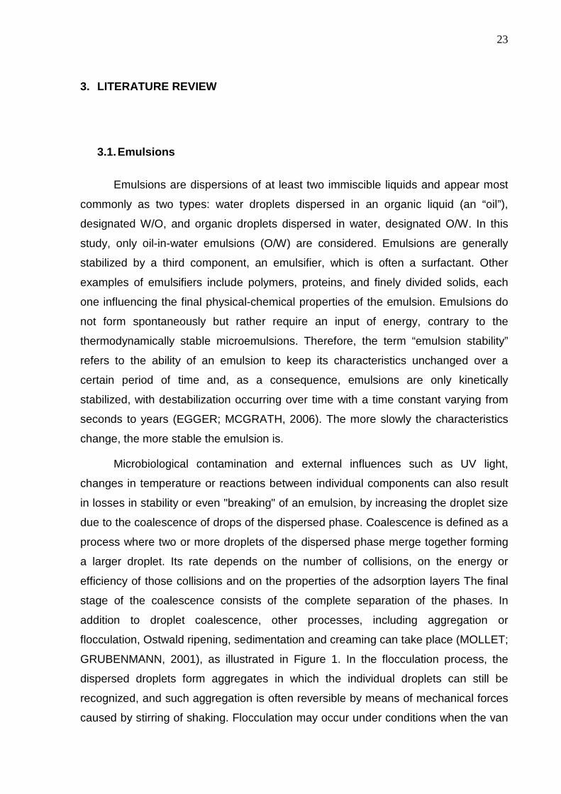
Microbiological contamination and external influences such as UV light,
changes in temperature or reactions between individual components can also result
in losses in stability or even "breaking" of an emulsion, by increasing the droplet size
due to the coalescence of drops of the dispersed phase. Coalescence is defined as a
process where two or more droplets of the dispersed phase merge together forming
a larger droplet. Its rate depends on the number of collisions, on the energy or
efficiency of those collisions and on the properties of the adsorption layers The final
stage of the coalescence consists of the complete separation of the phases. In
addition to droplet coalescence, other processes, including aggregation or
flocculation, Ostwald ripening, sedimentation and creaming can take place (MOLLET;
GRUBENMANN, 2001), as illustrated in Figure 1. In the flocculation process, the
dispersed droplets form aggregates in which the individual droplets can still be
recognized, and such aggregation is often reversible by means of mechanical forces
caused by stirring of shaking. Flocculation may occur under conditions when the van

24
der Waals attractive energy exceeds the repulsive energy and can be weak or
strong, depending on the strength of inter-drop forces. It can cause local
concentration differences within the emulsion due to the change of the droplet size
distribution and often results in coalescence. While aggregation is a reversible
process, coalescence is irreversible. Ostwald ripening refers to the mass diffusion of
several small droplets that ceases to exist and their mass is added to a few larger
drops. Creaming is an upward migration phenomenon due to the density difference
between disperse and continuous phases (HARUSAWA; MITSUI, 1975). Different
processes can occur simultaneously.
In this study, since the droplets of the evaluated emulsions are typically small
and they can not be considered as highly concentrated systems, the ripening
phenomenon is not significant (CHISTYAKOV, 2001; VARGAS, 2014). Besides,
some exploratory evaluations of commercial MWFs artificially aged with CaCl2, using
an optical scanning turbidimeter, Turbiscan Lab Expert® (from Formulaction), have
shown profiles typical of particle size variation, like coalescence process, as
illustrated in Figure 2. Thus, in this study, only the coalescence is considered as a
cause of emulsion destabilization.
Figure 1: Illustration of the emulsion destabilization processes (MOLLET;
GRUBENMANN, 2001).

25
Figure 2: Illustration of the obtained profile of a commercial MWF during artificial
aging with CaCl2, using an optical scanning turbidimeter.
The stability of an emulsion depends on several factors, some of which are
size distribution of the dispersed phase, the volume fraction of the dispersed phase
and the type and quantity of the surfactant that, depending on the mechanism
involved, promotes steric stabilization of the system or affect the repulsion forces
between droplets of the dispersed phase. For this this factor, its dependency is
explained by the DLVO Theory, proposed by Derjaguin and Landau and by Verwey
and Overbeek (HIEMENZ; RAJAGOPALAN, 1997), by which it is possible to estimate
the total interaction energy and the energy gap for coalescence or coagulation to
occur. Otherwise, when the stabilization is steric, which is most likely the stabilization
mechanism in the MWFs of this study, there are a formation of an adsorbed layer in
the surface of the droplets, causing steric repulsion, which prevent the close
approach of dispersed phase droplets (WILDE, 2000).
The size distribution of the dispersed phase affects the emulsion stability
because it is related to the free-energy change in the coalescence of two droplets,
which can be calculated by the product of the surface tension by the variation of the
surface area, at constant volume, temperature, composition and surface tension.
The area decreases as droplets coalesce, hence the change in the free-energy of the
system is negative and the coalescence is therefore spontaneous. The larger the
droplets, the larger is the surface area reduction, and more spontaneous is the
coalescence process, and, therefore, less stable is the emulsion (MORRISON;
ROSS, 2002). So, an increase in the droplet size of an emulsion is an indicator of its
partial destabilization.

26
3.2. Metalworking Fluid Emulsions
Metalworking fluids are also known as “cutting and grinding fluids”,
“metalforming fluids” or simply as “coolants”, but their function goes far beyond
cooling: they transport the chips generated in the process away from the cutting
zone, help to prevent rewelding and corrosion, reduce the power required to machine
a given material, extend tool life, increase productivity, help to generate chips with
specific properties, and are responsible for the cooling and lubrication (BYERS,
2006). They are not only used for machining metals, but can also be used for
machining plastics, ceramics, glass and other materials.
These fluids can be classified as pure oils, soluble oils, semisynthetics and
synthetics. Soluble oils are in fact O/W emulsions made from mineral or synthetic oils
and constitute the largest amount of fluid used in metalworking – they are also the
focus of this study. Usually they are sold as concentrated emulsions to be diluted in
factory facilities, before filling up the machines. Typical dilution ratios for general
machining and grinding are 1%-20% in water, with 5% being the most common
dilution level (BYERS, 2006).
The major component of soluble oils is either a naphthenic or a paraffinic oil in
usual concentrations of 40%-85%. Naphthenic oils have been predominantly used
because of their historically lower cost and ease of emulsification. Vegetable based
oils may also be used to prepare a water-dilutable emulsion for metalworking, but
they have higher costs, larger tendency to undergo oxidation and hydrolysis
reactions, and microbial growth issues. One favorable aspect related to the use of
vegetable oils is that they are biodegradable, resulting in less environmental
problems involved in waste destination.
Besides the oil and the water, there are several other components in MWF
emulsions. The formulations are usually complex in order to ensure that the fluid has
all the properties needed for machining, as well as chemical and microbiological
stability. Several additives are added to fulfill the purpose of emulsification, corrosion
inhibition, lubrication, microbial control, pH buffering, coupling, defoaming, dispersing

27
and wetting. While more than 300 different components can take part in the
formulation of MWF emulsions, a single mixture may contain up to 60 different
components (BRINKSMEIER et al., 2009; GLASSE et al., 2012). All additives are
chosen according to the process and material type, so there is an infinite number of
possible formulations.
In the so-called soluble oils, i.e., MWF emulsions, emulsion stability is the
most critical attribute (BYERS, 2006), because losses in stability would affect all
other fluid characteristics, like lubricating and cooling. Changes in droplet size, even
in its first stages, can decrease the performance of the MWF and thereby cause
several problems in machining processes, such as reduction of tool life, corrosion,
foam formation and others (EL BARADIE, 1996). Consequently, emulsifiers and
other additives are chosen carefully to guarantee the stability of the fluid for as long
as possible. As previously mentioned, the droplet size is an important property,
because it has large influence on stability (ABISMAÏL et al., 1999; CHANAMAI;
MCCLEMENTS, 2000; DICKINSON, 1992). The size of the emulsion particles also
determines its appearance: normal “milky” emulsions have particle sizes of
approximately 2.0 to 50 μm in mean diameter and micro-like emulsions are
translucent solutions and have particle sizes of 0.1 to 2.0 μm 1(BYERS, 2006).
However, the droplet size range of an emulsion changes over time.
In machining processes there is a high rate of heat generation and it is
estimated that about 10% of the heat produced is removed by the fluid, 80% by the
chips, and 10% is dissipated over the tool. With time, this thermal stress can lead to
partial degradation of emulsifiers and other additives, favoring microbiological
contamination, which also contributes to degradation of emulsion components and its
stability reduction, changing the droplet size profile over time (BRINKSMEIER et al.,
2009; BYERS, 2006). The increase in droplet size over time is defined as the “aging”
of an emulsion. At a certain stage of this destabilization process, the fluid is
considered “old” or “aged” and is disposed.
Zimmerman et al. (2003) have found that a particle size shift from 20 to 2000
nm in a commercial MWF resulted in a 440% increase in microbial load during a 48-h
1 The presented nomenclature for emulsion classification is typical of MWFs. Therefore, other types of emulsions may receive a different classification for different particle size range.

28
inoculation, leading to the release of acids, lowering pH, and further increasing
particle size. As this process continues, it can ultimately lead to oil-water phase
separation.
Even though emulsion stability is critical in manufacturing processes and,
consequently, monitoring is a key issue, for MWF it is normally carried out only by
what is required in local legislations, like periodic measurements of oil concentration
(since fluid concentration changes over time due to water evaporation), pH, viscosity
and contamination. In this way, changes in fluid characteristics usually are detected
only when the destabilization of the emulsion is already significant, leading to
problems in machining processes, decreasing tool life, among others. In other
occasions, fluids with no loss of performance are disposed because some of these
measurements have reached the stipulated limit. In both situations, it has a
significant impact on costs for this industry sector. This is why Greeley and
Rajagopalan (2004) suggest that the evaluation of emulsion destabilization could be
possibly used as a better indicator for monitoring the quality of MWF.
Concerning the droplet size distribution (DSD), Figure 3 shows typical DSD
curves of a fresh metalworking fluid, a metalworking fluid in use and an aged
metalworking fluid. Due to this change in the distribution pattern, real-time monitoring
of the DSD can be used as a more suitable and sensitive method than conventional
techniques to detect changes in characteristics of these emulsions. This can be
done, for example, by light scattering techniques, as discussed in later chapters.
In this study two types of oil-in-water emulsions were evaluated: rapeseed oil
emulsions and commercial metalworking fluids. Rapeseed oil is one of the oils used
in some MWF formulations. An emulsion prepared with this oil, emulsifier and water
constitutes a relatively simple system to evaluate the proposed technique before
applying it in more complex commercial fluids.

29
Figure 3: Illustration of changes in droplet size distribution of a typical MWF due to
emulsion aging.
3.3. Methods for the Monitoring of Emulsion Destabi lization Process
3.3.1. Conventional Methods
An indication of the thermodynamic work involved in creating an emulsion is
provided by the area of interface produced. As the emulsion ages, the area of
interface decreases (MORRISON; ROSS, 2002), and this decrease means that the
size of droplets in the emulsion increase. Thus, emulsion stability (or emulsion
destabilization) can be monitored by measuring the change in droplet size.
A direct way to estimate the average droplet size consists of examining the
emulsion in a microscope. This involves placing a sample in the viewing area of a
microscope, where an image can be captured and image analysis software can be
used to extract a size-frequency distribution. The system studied needs to be
transparent to light, which may require dilution of the emulsion. In addition, this
technique produces a 2D image of the emulsion, which may affect the accuracy of
the results. The number of droplets sampled is also small, unless a large number of
repeated measurements are made. Confocal microscopy can be used to produce 3D
images of emulsion droplets. However, in the absence of refractive index matching of

30
the continuous and discontinuous phases, this measurement is limited to the top
layer of droplets (CHESTNUT, 1997).
Another method used for measuring droplet size is by means of ionic
conductivity. The electrical conductivity of an emulsion depends on the concentration
of the dispersed oil phase. An unstable emulsion can have a variation in the
concentration of the dispersed oil droplets from bottom to top. Therefore, the stability
of an emulsion can be checked by comparing the electrical conductivity at the top
and the bottom of the container. In a different method, the conductivity
measurements can be based on the effect of caused by a droplet passing through a
small orifice, on either side of which is an electrical contact. For the case of an O/W
emulsion, when the oil droplet passes through the orifice, there is a dip in the
conductivity of the material that can be related to the droplet size. These methods
can not always be applied to concentrated emulsions and often require an electrolyte
to be added to the aqueous phase in order to enhance conductivity contrast, which
may affect emulsion stability. In addition, the high shear in the orifice can cause
further emulsion droplet break-up (JOHNS; HOLLINGSWORTH, 2007).
Acoustic methods are based on the fact that the speed of sound in an
emulsion depends on the concentration of the dispersed oil phase. This speed is
measured by transmitting a short pulse of sound and measuring the time required for
the pulse to reach a detector opposite to the source. The advantage of determining
emulsion stability by this method is that the sample can be measured without dilution,
even for relatively concentrated emulsions, typically up to 30% (volume basis), and
the container and the sample can be optically opaque. However, large errors can be
caused by the presence of tiny gas bubbles. A large number of thermo-physical
properties of both the continuous and discontinuous phases are required for the
experimental data inversion procedure (COUPLAND; JULIAN MCCLEMENTS, 2001;
MCCLEMENTS; COUPLAND, 1996).
Nuclear Magnetic Resonance (NMR) techniques can be used to measure
droplet sizes in the range between 50 nm and 20 mm in concentrated emulsions
which are opaque and contaminated with other materials (e.g. gas bubbles and
suspended solids). NMR is generally able to measure an emulsion DSD via the
application of magnetic field gradients; such gradients are also able to image
31
emulsion macroscopic structure as well as the velocity field of flowing emulsions.
They are non-invasive techniques that have the advantage of requiring little sample
preparation, but that are not yet established as a standard technique for o/w
emulsions despite the fact that the principle of the measurement is not new. This is
caused by technical limitations, mainly with respect to the size range of droplets that
can be accurately sized, and by the fact that it often requires expensive equipments,
making the technique unavailable for routine measurements in a practical sense
(HOLLINGSWORTH et al., 2004; JOHNS; HOLLINGSWORTH, 2007; KIOKIAS;
RESZKA; BOT, 2004).
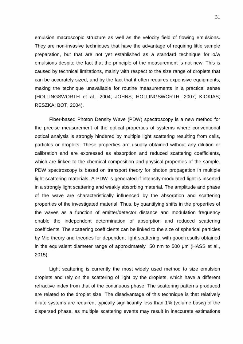
Fiber-based Photon Density Wave (PDW) spectroscopy is a new method for
the precise measurement of the optical properties of systems where conventional
optical analysis is strongly hindered by multiple light scattering resulting from cells,
particles or droplets. These properties are usually obtained without any dilution or
calibration and are expressed as absorption and reduced scattering coefficients,
which are linked to the chemical composition and physical properties of the sample.
PDW spectroscopy is based on transport theory for photon propagation in multiple
light scattering materials. A PDW is generated if intensity-modulated light is inserted
in a strongly light scattering and weakly absorbing material. The amplitude and phase
of the wave are characteristically influenced by the absorption and scattering
properties of the investigated material. Thus, by quantifying shifts in the properties of
the waves as a function of emitter/detector distance and modulation frequency
enable the independent determination of absorption and reduced scattering
coefficients. The scattering coefficients can be linked to the size of spherical particles
by Mie theory and theories for dependent light scattering, with good results obtained
in the equivalent diameter range of approximately 50 nm to 500 µm (HASS et al.,
2015).
Light scattering is currently the most widely used method to size emulsion
droplets and rely on the scattering of light by the droplets, which have a different
refractive index from that of the continuous phase. The scattering patterns produced
are related to the droplet size. The disadvantage of this technique is that relatively
dilute systems are required, typically significantly less than 1% (volume basis) of the
dispersed phase, as multiple scattering events may result in inaccurate estimations

32
of droplet size. The method also requires that the sample be reasonably transparent.
The technique is flexible in that it can measure a wide range of droplet sizes, typically
between 20nm and 2000 μm (COUPLAND; JULIAN MCCLEMENTS, 2001; JOHNS;
HOLLINGSWORTH, 2007; NOVALES et al., 2003).
Although there are many available methods for emulsion stability evaluation,
hardly any one of them is used for evaluation of MWF in machining processes. Some
of them require expensive equipment; while others are difficult to be implemented
under machining process conditions. New fluids have their stability evaluated only by
standard methods (ASTM D3707 and ASTM D3709), which involve storage under
special conditions for a certain period of time and, after that, phase separation is
visually evaluated. In some cases, droplet size is also measured by light scattering
methods, but only for new fluids. When in use, the controls are much simpler: only
what is required in local legislation and visual changes, including visual phase
separation.
3.3.2. Application of UV/VIS Spectroscopy and Optic al Models
When a beam of light incides on a particle, the electrons of the particle are
excited into oscillatory motion. The excited electric charges re-emit energy in all
directions (scattering) and may convert a part of the incident radiation into thermal
energy (absorption). The sum of both, scattering and absorption is called extinction.
Depending on the chemical species, and on the energy of the incident light,
scattering can be elastic or inelastic (like Raman scattering).
Extinction by an individual particle depends on its size, refractive index and
shape, and the wavelength of the incident light. For a typical DSD in emulsions, the
most suitable optical models for treatment of spectroscopic data are based on the
Mie theory (MIE, 1908). This model enables to estimate the light scattering patterns
for light sources with given properties interacting with spherical particles of known
size and optical properties dispersed in a medium with known optical properties.

33
Detailed descriptions of the Mie model can be found, for example, in Bohren and
Huffman (1983).
Thus, when a suspension of spherical particles of known refractive index is
illuminated with light of different wavelengths, the resulting optical spectral extinction
contains information that, in principle, can be used to estimate the particle size
distribution of the suspended particles.
A number of papers have been published in recent years, showing the
application of UV/Vis spectroscopy to obtain information on the DSD and stability of
emulsions (e.g. ASSENHAIMER et al., 2014; CELIS; GARCIA-RUBIO, 2002, 2008;
DELUHERY; RAJAGOPALAN, 2005; ELICABE; GARCIA-RUBIO, 1990; GLASSE et
al., 2013, 2014).
Song et al. (2000) used spectroscopic measurements in a method called
Turbidity Ratio for comparing stabilities of different emulsions. Deluhery and
Rajagopalan (2005) proposed a method for rapid evaluation of MWF stability, by
modifying the Turbidity Ratio method and establishing a stability coefficient called
Wavelength Exponent (z). This coefficient was also based on the work of Reddy and
Fogler (1981) and on the Mie Theory (MIE, 1908), and can be used to estimate
stability of emulsions with nearly mono-disperse population of non-absorbing spheres
by evaluating time-changes in the measured spectra.
Equation 1 relates the measured turbidity τ(λ) via spectrometry with the optical
path length L, the emitted light intensity, I0, and the received light intensity I, for light
with wavelength λ. The term ln(I0/I) is referred to the absorbance or extinction.
���� = �� � ��� (1)

34
From the Mie Theory, the turbidity, τ(λ), can be related to the particle size2 (x)
by means of Equation 2, where f(x) is the DSD density function, Np is the total particle
number per unit volume of the system, and Qext is the extinction efficiency, obtained
from the Mie model.
���� = �� �� � ������, ����������∞� (2)
The extinction of light by emulsions is the result of light absorption by the
continuous and dispersed phases plus scattering. For a nonabsorbing system, the
turbidity can be directly related to scattering by the suspended droplets. The
extinction efficiency Qext depends on the particle size parameter and the refractive
index of both phases, evaluated at λ. For dilute dispersions consisting of
monodisperse spherical nonabsorbing particles significantly smaller than the
wavelength of the incident light, scattering is described by the Rayleigh scattering
regime (BOHREN, C.F., HUFFMAN, 1983). Under this regime, and if it is assumed
that the refractive index ratio does not depend significantly on the wavelength, which
usually is a good approximation for such systems, Qext can be expressed in a
simplified form (REDDY; FOGLER, 1981), as shown in Equation 3, where the
parameter k” is the size-independent component that incorporates the properties
contained in the expression for the scattering coefficient under the Rayleigh
scattering regime, λ is the wavelength and z is the exponent of the wavelength, λ,
dependent on particle size and refractive index.
���� = �". �! "
(3)
2 The size parameter x can be defined as the particle diameter, but some authors prefer to define it as the particle radius,
making the proper adjustments in the corresponding equations.

35
For this same dispersion of monodisperse spherical nonabsorbing particles,
Equation 2 can be simplified and rewritten as Equation 4.
���� = �� �� ���" �
! " (4)
Under Rayleigh regime, the exponent z is equal to 4 (BOHREN, C.F.,
HUFFMAN, 1983) and decreases as the particle size increases. Note that the only
variables in this equation are the size parameter x, the exponent z, the turbidity τ(λ)
and the wavelength λ. Thus, for a given particle diameter, i.e., if x is constant, the
wavelength exponent z can be expressed as the slope of ln(τ) versus ln(1/λ), as
indicated in Equation 5.
# = $%&'�(�)$*&'+, - (5)
Therefore, under the mentioned assumptions, the wavelength exponent for a
given emulsion can be determined from turbidity measurements at different values of
λ by fitting Equation 5 to the data.
The same concept can also be applied to other particle systems, e.g. aerosols.
However, in the study of the particle size of aerosols, the exponent of the wavelength
is called Angstrom Exponent (å) and some additional restrictions are imposed in its
definition, like the assumption of a homogeneous atmospheric layer, where the
aerosol is distributed uniformly over the ranges of altitudes (ANGSTRÖM, 1930;
JUNG; KIM, 2010; SEINFELD; PANDIS, 2006).
Because of its dependency on particle size, Deluhery and Rajagopalan (2005)
used the wavelength exponent z as an indicator of emulsion stability. In their paper,

36
the decrease in the exponent over time is related to the destabilization of emulsions
by associating this process with the increase in droplet size by coalescence.
This author and the team of researchers in the BRAGECRIM project
generalized the application of this method, showing that, although the wavelength
exponent is in its definition valid for monodisperse systems only, it can also be used
for evaluation of stability of polydisperse systems, with monomodal and even bimodal
distributions (GLASSE et al., 2013). In addition to that, we have also shown that
there is no need to exclusively evaluate time-changes in the spectra, as proposed by
Deluhery and Rajagopalan (2005), since the emulsion stability can also be evaluated
by performing instantaneous measurement of turbidity and evaluating the quality of
the fitting of the corresponding correlations. Although the use of the wavelength
exponent for emulsion stability (or destabilization) evaluation is easy to be
implemented, it performs not so well when applied to droplet populations with high
polydispersity or above a certain range of droplet diameter. Figure 4 exemplifies the
simulated behavior of the wavelength exponent with the increase of droplet diameter
for a monodisperse distribution; there is a decrease in z values with the increase of
the diameter. However, between 1 μm and 10 μm it increases again, with oscillatory
behavior. Therefore, it was not chosen in this study as the method of MWF quality
evaluation, but it was used as an auxiliary method, with other techniques, for
comparison.
Figure 4: Illustration of the simulated behavior of the wavelength exponent z versus
the droplet size of a monodispersed distribution (GLASSE, 2015).

37
In a different approach Celis and Garcia-Rubio (2002, 2008, 2004) and Celis
et al. (2008) used spectroscopic data treated by optical models and inversion
methods using regularization to obtain information on the DSD of a dispersed system
in which the time variation of the extinction pattern can be correlated with properties
of the emulsion. Most of these models were also based on the Mie Theory.
Eliçabe and Garcia-Rubio (1990) used an algorithm based on optical models
to estimate the DSD in emulsions and dispersions based on the optical properties of
its components and on spectroscopic measurements and inversion methods. The
method enables the acquisition of real-time data, enabling in-line monitoring of DSD
in emulsions. In the model proposed by the authors, by defining the function K as
.��, �� ≡ �� ������, ����, (6)
then Equation 2 can be identified as a Fredholm integral equation of the first kind, in
which K(λ,x) is the corresponding Kernel and the numerical solution can be found by
using an appropriate discrete model. If the integrand in this equation is discretized
into (n-1) intervals, the integral can be approximated at a given wavelength λi with a
sum,
�0 = ∑ 203 �3'34� (7)
where:
�0 ≡ ���0� , i = 1, 2, …m (8)
�3 ≡ ���3� , j = 1, 2, …n (9)

38
203 = �∆� ∑ .0����∆��6�67+ − �67+∆� ∑ .0���∆��6�67+ + �6:+∆� ∑ .0���∆��6:+�6 − �
∆� ∑ .0����∆��6:+�6 ,
j = 2, 3, ...n-1 (10)
20� = �;∆� ∑ .0���∆��;�+ − �∆� ∑ .0����∆��;�+ (11)
20' = �∆� ∑ .0����∆��<�<7+ − �<7+∆� ∑ .0���∆��<�<7+ (12)
The details of the discretization procedure are given in the referenced paper.
The Kernels can be calculated by the Mie theory with the corresponding equations
presented, for instance, in Bohren and Huffman (1983).
If the extinction is evaluated at m wavelengths, λi, i=1, 2, …m, then Equation 7
can be written in matrix form as
�̅ = >̿� ̅ (13)
where
�̅ = @ ��…�BC , >̿ = D203E , �̅ = @��…�'
C
If quadrature and measurement errors are considered, Equation 13 can be
rewritten as the following equation.
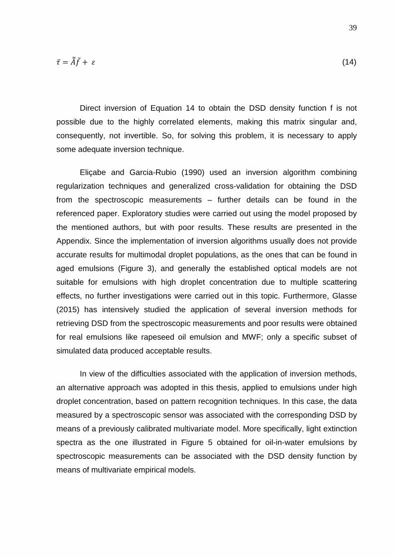
39
�̅ = >̿�̅ + F (14)
Direct inversion of Equation 14 to obtain the DSD density function f is not
possible due to the highly correlated elements, making this matrix singular and,
consequently, not invertible. So, for solving this problem, it is necessary to apply
some adequate inversion technique.
Eliçabe and Garcia-Rubio (1990) used an inversion algorithm combining
regularization techniques and generalized cross-validation for obtaining the DSD
from the spectroscopic measurements – further details can be found in the
referenced paper. Exploratory studies were carried out using the model proposed by
the mentioned authors, but with poor results. These results are presented in the
Appendix. Since the implementation of inversion algorithms usually does not provide
accurate results for multimodal droplet populations, as the ones that can be found in
aged emulsions (Figure 3), and generally the established optical models are not
suitable for emulsions with high droplet concentration due to multiple scattering
effects, no further investigations were carried out in this topic. Furthermore, Glasse
(2015) has intensively studied the application of several inversion methods for
retrieving DSD from the spectroscopic measurements and poor results were obtained
for real emulsions like rapeseed oil emulsion and MWF; only a specific subset of
simulated data produced acceptable results.
In view of the difficulties associated with the application of inversion methods,
an alternative approach was adopted in this thesis, applied to emulsions under high
droplet concentration, based on pattern recognition techniques. In this case, the data
measured by a spectroscopic sensor was associated with the corresponding DSD by
means of a previously calibrated multivariate model. More specifically, light extinction
spectra as the one illustrated in Figure 5 obtained for oil-in-water emulsions by
spectroscopic measurements can be associated with the DSD density function by
means of multivariate empirical models.

40
Figure 5: Example of a light extinction spectrum.
Among different techniques that can be applied, non-linear models such as
neural networks have been successfully applied in place of light scattering models to
estimate particle size distributions in concentrated solid-liquid suspensions
(GUARDANI; NASCIMENTO; ONIMARU, 2002; NASCIMENTO; GUARDANI;
GIULETTI, 1997) and to predict the stability of suspensions (VIÉ; JOHANNET;
AZÉMA, 2014). Thus, neural networks model were adopted in this thesis to associate
light extinction spectra with the DSD.

41
4. MATERIALS AND METHODS
4.1. Materials
The experiments reported in this text were carried out at the University of
Bremen by this author with the support of the German team of the BRAGECRIM joint
project. In this study rapeseed oil emulsions as well as commercial metalworking
fluids were evaluated. Rapeseed oil is one of the possible oils used in metalworking
fluids. An emulsion prepared with this oil, emulsifier and water constitutes a simple
system to evaluate the technique before applying it to more complex commercial
fluids. Rapeseed oil emulsions were prepared in laboratory, with different droplet
sizes, thus simulating both new and aged emulsions. For the MWF, aging was
simulated in the laboratory by adding CaCl2 to the system in order to disturb the
interface layer and thus enable droplet coalescence. For evaluation of MWF aging in
machining application, thus simulating a real-case scenario, no further treatment was
carried out besides dilution for achieving the recommended concentration.
4.1.1. Rapeseed Oil Emulsions
For the preparation of oil-in-water emulsions a commercial rapeseed oil was
used (from the German company Edeka, density 0,92 g/mL, refraction index 1.47).
The volume of the samples was 30 mL and the mass fraction of oil in the emulsions
ranged from 0.06% to 1.59%. Other substances used in the experiments were an
emulsifier, Polysorbate 80 (Tween 80, HLB 15, from Alfa Aesar, 0.07% to 0.42%),
and deionized water.
In the emulsification, an ultrasound equipment by Bandelin (Sonopuls HD 200,
with deep probe Sonopuls Kegelspitze KE76) was used. The intensity was set at
50% of the maximum for 1 to 5 minutes. The temperature variation was monitored

42
and used to estimate the dissipated energy in ultrasound emulsification by means of
Equation 15, where ρ is the density of the dispersed or continuous phases, φ is the
volumetric fraction of the dispersed phase, cp is the specific heat capacity and ∆T is
the measured temperature difference of the fluid before and after the sonication. The
initial temperatures of the samples was 20±1°C and typical ∆T of the emulsions were
in the range of 10°C to 50ºC, varying according to the sonication time. A total of 105
formulations were prepared by this method.
GH = IJKLLMN = %O. P$ . Q�,$ + �1 − O�. PS . Q�,S). ∆T. (15)
4.1.2. Metalworking Fluids
4.1.2.1. Artificial Aging
Commercial metalworking fluid, Kompakt YV Neu (oil concentration of
approximately 40 wt.%, density 0,96 g/mL, refraction index 1.25), was obtained from
Jokisch GmbH and prepared by dilution with deionized water to reach the MWF
desired concentrations (3.5 - 5.2 wt.%). Artificial aging, i.e., partial chemical
destabilization, was promoted by adding to the emulsions 0 - 0.3 wt.% of CaCl2
(CaCl2 .2H2O, purity of 99.5%), from Grüssing GmbH. This salt was chosen because
its presence is common in hard water used in machining facilities in Germany, where
the tests were conducted, and poses as a problem precisely for accelerating the
aging of the MWF diluted with this water. A total of 104 formulations were prepared
by this method.

43
Figure 6: Chromatogram of MWF Kompakt YV Neu obtained by Gas
Chromatography–Mass Spectrometry analysis in a GCMS-QP2010 chromatograph.
Although it was not possible to have access to fluid formulation, GC-MS (Gas
Chromatography–Mass Spectrometry) analysis was performed in a GCMS-QP2010
chromatograph, from Shimadzu, for characterization purposes only. The resulting
chromatogram is presented in Figure 6, where is shown over 60 substances used in
the formulation of this fluid. The chemistry of metalworking fluids is as diverse as its

44
applications. Each formulating chemist develops his own fluid formula to meet the
performance criteria of the metalworking operation; however additives with function
of surfactants, biocides, emulsifiers and waxes are always present in the formulation.
Analyzing the main peaks of the chromatogram, it is possible to identify some of
these substances and its function in the MWF formulation: 2-phenoxiethanol
(biocidal); 3-octadecyloxy-1-propanol, 3-octadecyloxy-1-propanol and cis-9-
tetradecen-1-ol (emulsifiers); 1-dodecanol and 2-dodecyloxy-ethanol (surfactants); E-
9-eicosene (lubricant); 1-octadecene (dispersant); heneicosane (paraffin wax).
For the experiments aimed at applying the spectroscopic sensor and the
neural network model to the monitoring of MWF aging, 0.3 wt.% of CaCl2 was added
to metalworking fluid emulsions with concentration of 4 wt.% and the aging was
monitored over time.
4.1.2.2. Machining Application
In the last stage of the experiments, a campaign was carried out aimed at
obtaining data as near as possible of a real case scenario. In this campaign, a total of
7 different commercial metalworking fluids (Acmosit 65-66, from Acmos Chemie KG;
Grindex 10, from Blaser Swisslube; Unimet 230 BF, from Oemeta; Rhenus r.meta TS
42, Rhenus XY 121 HM and Rhenus R-Flex, from Rhenus Lub; Zubora 10 M Extra,
from Zeller-Gmelin) were monitored for a period of 13 months while they were used
in 3 different machines in a machining facility at the University of Bremen (a vertical
turning machine, Index C200-4D, a precision milling machine, Sauer 20 Linear, and a
cylindrical grinding machine, Overbeck 600 R-CNC). All these MWF samples are oil-
in-water emulsions, made from synthetic oils and several additives to fulfill the
purpose of emulsification, corrosion inhibition, microbial control, among others. Each
emulsion was previously diluted to the recommended concentration for each
corresponding application. Once the fluid loses water due to evaporation during the
process, some adjustments in concentration where carried out over time.

45
4.2. Measurements
4.2.1. Spectroscopic Measurements
Light extinction spectra measurements were performed in all samples with a
UV-Vis-NIR spectrometer, model HR2000+ES, from OceanOptics, with light source
DH 2000-BAL, spectral resolution of 0.5 nm, and a dip probe with 6.35 mm diameter,
127 mm of length and optical length of 2 mm, which enables in-line and real-time
monitoring (Figure 7). The dark noise and the reference signal were recorded prior to
measurement and subtracted from the measurement signal. Prior to the
measurements, the light source was warmed up for 30 min to reach full intensity.
Absorbance was measured for light wavelength in the range 200–1000 nm by probe
immersion in the samples.
Figure 7: Spectrometer with deep probe for in-line monitoring. Images at the
right: detail of deep probe.
4.2.2. Reference Measurements: Droplet Size Distrib ution
The evaluation of the droplet size distribution for neural network calibration
was based on measurements with a Malvern Mastersizer 2000 laser diffractometer,
with particle size detection range from 0.02 to 2000 µm. The measurements of the
emulsion samples were performed using the universal model for spherical particles in
the measurement suite and the corresponding refractive index of each phase of the

46
emulsion. For each sample the mean values of the DSD from three consecutive runs
carried out over 35s were recorded.
Particle size analysis with Malvern Mastersizer is a well-established technique,
but the samples need to be diluted prior to the analysis in order to prevent multiple
scattering. Emulsion stability can be affected by dilution, although MWF formulations
should not be affected by that, especially considering that the manufacture
recommendation is for diluting it, within a certain range of concentration, before use.
However, in order to confirm that the dilution of the samples for analyzing the DSD
does not affect the result and can be trusted, a sample of the MWF Kompakt YV Neu
was left in the Malvern Mastersizer for 1h and the DSD was recorded in 1 min
intervals. Since no change in droplet size was observed during 1h (Figure 8), it is
safe to say that the dilution in the Malvern Mastersizer does not affect the stability of
the sample and this technique can be used for analyzing the DSD of MWF.
Figure 8: Evolution of particle size with time for MWF Kompakt YV Neu.
4.2.3. Wavelength Exponent
As previously mentioned, the extinction of light by emulsions is the result of
light absorption by the continuous and dispersed phases plus scattering. For a
nonabsorbing system, the turbidity can be directly related to scattering by the
suspended droplets and, therefore, can be directly related to the measured
absorbance of the emulsion. So, the exponent z can be found by measuring the

47
absorbance (Abs) of the emulsion at different wavelengths and determining the slope
of the ln(Abs) versus ln(1/λ) curves in a selected wavelength range (Figure 9).
Figure 9: Illustration of wavelength exponent calculation.
However, in order to use the wavelength exponent, it is necessary to assume
that there is no absorption in the selected wavelength range and that all the
measured absorbance is due to scattering. So, in order to choose the best range for
these evaluations, it was obtained from the supplier of this MWF the absorbance
spectrum of its main components, in different concentrations (Figure 10 and Figure
11). Not much information was provided about these measurements, but it was
possible to see the range of absorption of the main chemical species of the fluid prior
to emulsification, i.e., without interference of droplets scattering in absorbance
measurements. Based on this information, it is a good approximation to defined that
the best range to assume absence of absorption by the emulsion is from 400-700
nm. Thus, for the calculation of exponent z, it was chosen a 100nm interval in this
range, from 500 to 600nm, and all the fittings were carried out for this wavelength
range.
In the evaluation of MWF in machining application, the linear coefficient of the
fittings was also included in the collected data set. Although this coefficient itself does
not have a physical meaning, it is related to the concentration and optical properties
of the analyzed samples. Since it was not possible to have access to the optical
properties of the MWF in this part of the study, the linear coefficient of the fittings was

48
used in this evaluation to compensate this lack of information and to help differentiate
the data for different fluids.
Figure 10: Absorbance spectrum of main components of MWF Kompakt YV Neu, in
different concentrations (for components “A” to “F”).

49
Figure 11: Absorbance spectrum of main components of MWF Kompakt YV Neu, in
different concentrations (for components “G” to “J”).
4.2.4. Application to Long Term Monitoring of MWF D estabilization
For the evaluation of MWF in machining applications, periodic physical-
chemistry and microbiological analysis of the fluid (pH, oil concentration, nitrite
content and microbiological contamination by ATP method, according to German
regulation requirements in norm VDI 3397) were performed over time as a routine of
the facility’s employers, with supervision of the project team. Samples were collected
weekly during 13 months and the measurements were performed by the machining
operators in the laboratory facility. MWF also receive a classification in each analysis
according to the machine operator perception concerning the performance of the
MWF at the time when the samples were collected for analysis. The MWF samples
were thus classified according to their “status” in three classes: 1, or green (no signs
of deterioration), 2, or yellow (initial signs of deterioration), and 3, or red (high degree
of deterioration). Although the machine operator perception of quality not always
receives this qualitative classification in the facilities, generally it is one of the
determinant factors for deciding when a MWF can be considered aged and has to be

50
disposed and replaced. Spectroscopic measurements and analysis of DSD of all
collected samples were performed by the German team of the project, as previously
described.
4.3. Characterization Methods
4.3.1. Pattern Recognition Techniques: Artificial N eural Networks
An Artificial Neural Network (ANN) is a non-linear computational model based
on the structure and function of biological Neural Networks. Like human brain but in a
simpler level, ANN has the ability to recognize patterns and behaviors hidden in a
data set organized as inputs and outputs and to generalize it for similar observations.
Because of that it is said that these networks have the ability to “learn” about the
behavior of a given system and then simulate it.
The basic unit of an ANN is the neuron, an information-processing unit that is
fundamental to its operation. The manner in which these neurons are structured is
intimately linked with the learning algorithm used to train the network. In general
there are three different classes of network architecture: Single Layer Feedforward
Networks, Multilayer Feedforward Networks and Recurrent Networks (HAYKIN,
1999). In the first class, all the neurons are organized in the form of a layer and there
is an input layer of source nodes that projects onto an output layer of neurons, but
not vice-versa. The second type distinguishes itself from the first by the presence of
one or more hidden layers, whose computation nodes are correspondingly called
hidden neurons. By adding one or more hidden layers, the network is able to extract
higher order statistics. The last class of networks architecture distinguishes itself from
Feedforward Neural Networks in that it has at least one feedback loop. In this study,
only Multilayer Feedforward Networks were used. More specifically, a three layer
feedforward network was fit to the experimental data.

51
Neural networks have been applied to several systems of high complexity in
different fields where phenomenological modeling is not suitable or is difficult to be
implemented. In the field of this study, some examples of previous applications of the
method to retrieve particle size distribution from optical measurement methods
include the study by Guardani et al. (2002), who used ANN models to replace the
optical model and to obtain particle size distribution of three different suspensions
from forward light scattering measurements. The advantage is the possibility of
analysis of suspensions with higher concentrations, which cannot be accurately
measured by optical models due to multiple scattering phenomena.
Berdnik and Loiko (2006) and Berdnik et al. (2006) used ANN for retrieving
size and refractive index of spherical particles by angular dependence of scattered
light in scanning flow cytometry as an easier way for obtaining this information than
with the application of other methods involving the calculation of complex integrals or
trial-and-error methods.
In this thesis, multivariate models based on neural networks are used as an
alternative to optical models to associate spectroscopic measurements with DSD.
Thus, with the calibration of multivariate models, an association is established
between the extinction pattern and the DSD of a given emulsion system. This
approach provides a way to estimate the DSD in systems with high droplet
concentration, in which multiple scattering does not enable the application of optical
light scattering models.
Figure 12 shows an illustration of a three-layer feedforward neural network,
like the ones used in this study. To neuron i (i=1,2,...,q), located in layer j (j=1,2,3) of
a network, the received information Sj is a weighted sum of the inputs Xi by the
weights Wi,j (Equation 16). The last input, with value equal to 1, is a bias, which has
the effect of increasing or lowering the net input of the activation function, depending
on whether it is positive or negative, respectively. In this way, bias neurons may help
the neural network to learn patterns, by allowing it to output a value of zero even
when the input is near one.

52
U3 = ∑ V0,3W0 9 VXY�,3X04� (16)
The output from neuron j is a response function Z3 � �%U3), in which f(Sj) can
consist of different mathematical forms. In most cases a sigmoidal function is used
(Equation 17).
�%U3) � ��[�7\6 (17)
Figure 12: Illustration of a feed-forward neural network (ASSENHAIMER et al., 2014).
The fitting of a neural network consists of two steps: training, consisting of the
adjustment of the parameters, or weights, for a given neural network structure, and
validation. In the first part, known values of inputs and outputs are presented to the
network and the set of weights is selected so that a minimum squared error E
between calculated and observed values of the outputs is achieved. The squared
error E is defined in Equation 18, where yk is the experimental (observed) value and
Ok is the calculated value of output k. In this thesis the fitting was based on the
backpropagation algorithm (RUMMELHART, D., MCCLELLAND, 1986).

53
G = ∑ ∑ ]̂�B� − Z�̂B� ��̂4�_B4� (18)
The second part of the fitting consists of the validation of the model. The
calculated outputs are compared with experimental values of another set of
observations, which have not been used in the training step, in order to check if the
model is able to predict the desired results adequately.
The computational programs used in this work for neural network model fitting,
validation and simulations were developed in the Chemical Engineering Department,
Escola Politécnica, Universidade de São Paulo (USP).
4.3.1.1. Architecture of the ANN
The architecture of the network is very important to define its capacity of
convergence and generalization. The choice of a suitable architecture, with an
adequate number of parameters, is the main factor for the success of the data
training.
The number of neurons in the input and output layers is determined by the
problem structure. The difficulty is to find the ideal number of neurons in the hidden
layer. This number, sometimes, may be determined by rules as in Loesch and Sari
(TÁPIA, 2000, apud LOESCH and SARI, 1996), where “the number of neurons in the
hidden layer should be equal to the geometric mean of the number of inputs and
outputs”, or by the rule in Eberhart (TÁPIA, 2000, apud EBERHART, 1999), where
“the number of neurons in the hidden layer should be equal to the square root of the
sum of inputs and outputs”. Although these and other rules are sometimes suitable
for solving specific problems, they have not been proven to be reliable in all
applications. Thus, in most cases these rules can be adopted as a first estimation of
the number of neurons in the intermediary layer of a feed-forward neural network, but

54
the most adequate number must be based on fittings carried out for different values
of this parameter.
The higher is the number of neurons in the hidden layers, more complex will
be the network and large networks normally require large amounts of training data,
which may not be available. An analysis of the degree of freedom of an ANN
suggests that the number of observations available for training the network should be
higher than the number of parameters in the network, otherwise, significant overfitting
and poor generalization will be evident, which means that the error on the training set
is driven to a very small value, but when new data are presented to the network the
error is large; the network was successfully fitted to the data set, but it is unable to
generalize the fitted model for new data.
However, this is not necessarily true. Larger networks often result in lower
generalization error, even with a training set smaller that may be expected
(LAWRENCE; GILES; TSOI, 1997). The rule that states that “the number of
parameters in the network should be (significantly) less than the number of
examples” aim to prevent overfitting, but is unreliable as the optimal number of
parameters is likely to depend on other factors, e.g. the quality of the solution found,
the distribution of the data points, the amount of noise, and the nature of the function
being approximated. Specific rules, such as the above, are not commonly accurate.
In fact, larger networks may generalize well and better generalization is often
possible because they have less difficulty to find with local minima (LAWRENCE;
GILES; TSOI, 1997). This is also supported by the work of Bartlett (LAWRENCE;
GILES; TSOI, 1997, apud BARTLETT, 1996), who also found that neural networks
often perform successfully with training sets that are considerably smaller than the
number of network parameters, because it may be difficult to approximate the
training data with smaller networks. Nevertheless, some precautions may be taken
to confirm the absence of overfitting, like the removal of 20% to 30% of the data,
which is not used in the training step of the network, to validate the fitting of the
model. This step may be incorporated in the algorithm used for the fitting of the ANN
in order to minimize simultaneously the error of the testing set and the validation set.
If good results are found in the validation set, the hypothesis of overfitting can be
discarded.
55
In this study, the most adequate number of neurons in the hidden layer was
determined based on fittings carried out for different values of this parameter and
30% of all data were used exclusively for the validation of the model, as explained in
Chapter 4.3.1.
4.3.1.2. Holdback Input Randomization Method (HIPR method)
As shown in Figure 12, the structure of ANN models is characterized by the
fact that the information provided by each input is distributed in a weighed among all
neurons of successive layers. Thus, no model parameter is individually connected to
a specific input variable, which hinders the evaluation of the relative importance of
the ANN input variables. In view of this characteristic of ANN models, Kemp, Zaradic
and Hansen (2007) proposed a method based on a sequential randomized
perturbances in the input variables to determine the relative proportion to which each
input variable contributes to the predictive ability of the ANN model in the evaluated
range. This method was named by the authors Holdback Input Randomization
Method, or HIPR method.
In the HIPR method, the data are divided into a learning set, a validation set
and a test set following the ratio 3:1:1. The ANN is adjusted with data from the
learning set in the conventional way, and afterwards the error in relation to the
validation set is computed. The test set is used to calculate the error of the model
and thus to estimate the overall training success of the net. After the model is
adjusted and the error of the model is evaluated, then, according to the HIPR
method, each individual input variable is randomly varied within its range of validity
and sequentially, and the mean squared error (MSE) is computed for all random
values of each individual input variable. The contribution of each input variable to the
predictive ability of the ANN model can be estimated based on how much it affects
the MSE, compared to the minimum MSE value obtained in the model fitting step.
The procedure can be repeated a number of times in order to increase the
representativity of the test. The evaluation of the relative importance of each input

56
variable is thus based on the effect of the random perturbations on the MSE. If a
given input variable does not significantly contribute to the fitted model of the ANN,
then the MSE of the randomized data set will be close to the MSE relative to the
original data set. If a parameter contributes strongly to the fitted model of the ANN,
then the MSE of the data set in which this parameter is randomized will be larger
than the MSE relative to the original data set. This is a robust, simple, general
procedure for interpreting complex systems based on model performance, and the
results can be obtained without making any assumptions regarding the architecture
of the ANN model used.
An executable version of the algorithm developed by the author of this
method, using the C++ programming language, is available at
http://www.bio.upenn.edu/faculty/dunham/hipr/PennNN.zip. The evaluation of the
ANN models fitted in this study by the HIPR method was based on a computer
program in FORTRAN developed at the Department of Chemical Engineering,
Escola Politécnica, USP. More details about this method can be found in Kemp,
Zaradic and Hansen (2007).
4.3.2. Classification Techniques: Discriminant Anal ysis
Discrimination is a multivariate technique where distinct sets of observations
are separated and allocated in previously defined groups. As a separative procedure,
it is often employed in order to investigate observed differences when correlations
between observations from the data set are not well understood (JOHNSON;
WICHERN, 2007). The goal of this technique is to find “discriminants”, which consist
of quantitative criteria whose numerical values are used to separate variables or
observations as much as possible and, sometimes, to establish a rule that can be
used to optimally assign new observations to the labeled classes or groups. This
“discrimination” can be carried out by several different techniques, like the Test of
Hypothesis, the Linear Discriminant, the Quadratic Discriminant, the Fisher

57
Discriminant, among others. In this study, only linear and quadratic discriminant were
evaluated.
Considering two populations of observations xi, i =1,...n, with a priori
probabilities of occurrence p1 and p2, where `� + `� = 1, and considering that the
probability density functions f1(x) e f2(x) are as illustrated in Figure 13, then the
probability of a given observation x0, belonging to a group m, be designated to a
given group g, P(g|m), is expressed as Equation 19.
a�b|d� = a%�� ∈ fg|hB) = � �B�����ij (19)
Figure 13: Illustration of the distribution of observations between the groups
(GUARDANI; NASCIMENTO, 2007).
Thus, the probability of designating x0 to the wrong group is given by
a�2|1� = a��� ∈ f�|h�� = � �������i; (20)
a�1|2� = a��� ∈ f�|h�� = � �������i+ (21)
and the probability of designating x0 to the correct group is

58
a�1|1� = a��� ∈ f�|h�� = � �������i+ (22)
a�2|2� = a��� ∈ f�|h�� = � �������i; (23)
Therefore, these probabilities can be expressed as
a��� ∈ f�|h�� = a�1|1�. `�1� (24)
a��� ∈ f�|h�� = a�2|2�. `�2� (25)
when the observations are allocated in the correct group, and
a��� ∈ f�|h�� = a�2|1�. `�1� (26)
a��� ∈ f�|h�� = a�1|2�. `�2� (27)
when the observations are allocated in the wrong group.
“Costs” or “weights” may be assigned for misclassification, as shown in Table
1, and the Expected Cost of Misclassification, ECM, is defined as shown in Equation
28.
Table 1: Cost table for misclassification of the observations (GUARDANI; NASCIMENTO, 2007).
Classification Group G1 G2
G1 0 C(2|1) G2 C(1|2) 0
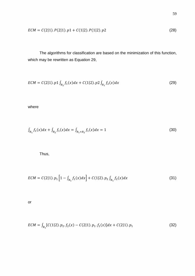
59
Glm = l�2|1�. a�2|1�. `1 9 l�1|2�. a�1|2�. `2 (28)
The algorithms for classification are based on the minimization of this function,
which may be rewritten as Equation 29,
Glm � l�2|1�. `1 � �������i;
9 l�1|2�. `2 � �������i+
(29)
where
� �������i+
9 � �������i;
� � �������i+Yi;
� 1 (30)
Thus,
Glm � l�2|1�. `� n1 − � �������i+
o 9 l�1|2�. `� � �������i+
(31)
or
Glm � � pl�1|2�. `�. ����� − l�2|1�. `�. �����q��i+
9 l�2|1�. `� (32)
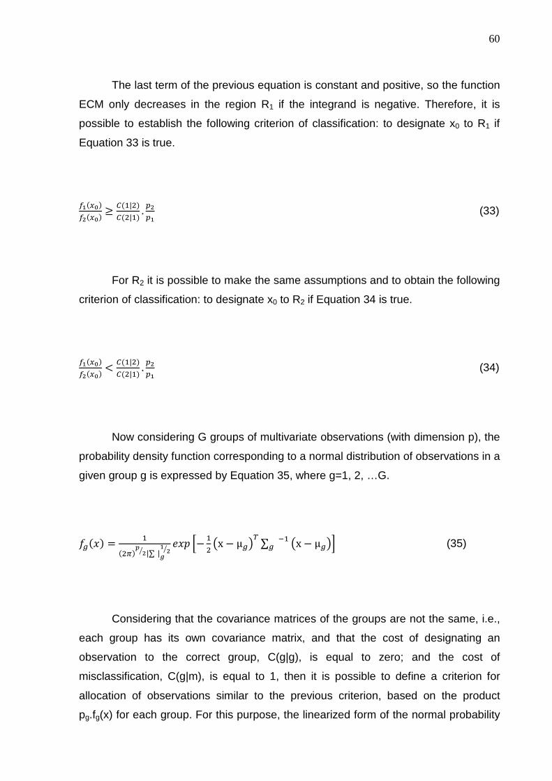
60
The last term of the previous equation is constant and positive, so the function
ECM only decreases in the region R1 if the integrand is negative. Therefore, it is
possible to establish the following criterion of classification: to designate x0 to R1 if
Equation 33 is true.
r+����r;���� ≥ t��|��
t��|�� . �;�+ (33)
For R2 it is possible to make the same assumptions and to obtain the following
criterion of classification: to designate x0 to R2 if Equation 34 is true.
r+����r;���� < t��|��
t��|�� . �;�+ (34)
Now considering G groups of multivariate observations (with dimension p), the
probability density function corresponding to a normal distribution of observations in a
given group g is expressed by Equation 35, where g=1, 2, …G.
�g��� = �����v ;w |∑ |j
+ ;w x�` n− �� %x − μg){ ∑ g [� %x − μg)o (35)
Considering that the covariance matrices of the groups are not the same, i.e.,
each group has its own covariance matrix, and that the cost of designating an
observation to the correct group, C(g|g), is equal to zero; and the cost of
misclassification, C(g|m), is equal to 1, then it is possible to define a criterion for
allocation of observations similar to the previous criterion, based on the product
pg.fg(x) for each group. For this purpose, the linearized form of the normal probability
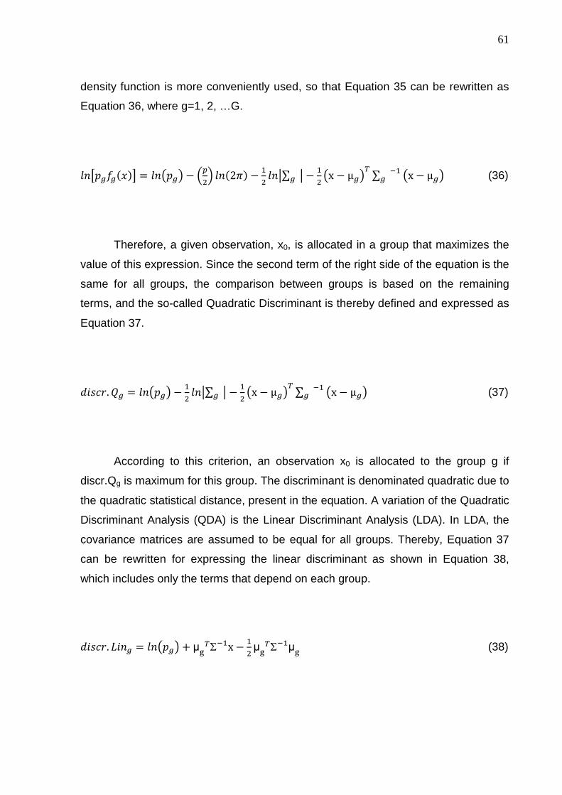
61
density function is more conveniently used, so that Equation 35 can be rewritten as
Equation 36, where g=1, 2, …G.
�|`g�g���} = �%`g) − �� ��2~� − �
� ��∑ g � − �� %x − μg){ ∑ g [� %x − μg) (36)
Therefore, a given observation, x0, is allocated in a group that maximizes the
value of this expression. Since the second term of the right side of the equation is the
same for all groups, the comparison between groups is based on the remaining
terms, and the so-called Quadratic Discriminant is thereby defined and expressed as
Equation 37.
���Q�. �g = �%`g) − �� ��∑ g � − �
� %x − μg){ ∑ g [� %x − μg) (37)
According to this criterion, an observation x0 is allocated to the group g if
discr.Qg is maximum for this group. The discriminant is denominated quadratic due to
the quadratic statistical distance, present in the equation. A variation of the Quadratic
Discriminant Analysis (QDA) is the Linear Discriminant Analysis (LDA). In LDA, the
covariance matrices are assumed to be equal for all groups. Thereby, Equation 37
can be rewritten for expressing the linear discriminant as shown in Equation 38,
which includes only the terms that depend on each group.
���Q�. ��g = �%`g) + µ�{Σ
[�x − ��µ�{
Σ[�µ� (38)

62
More detailed information about discriminant analysis can be found in Johnson
and Wichern (2007).
In this study, LDA and QDA were applied to the data using the statistical
software Minitab, for convenience. All evaluations were based on cross-validation,
which is a technique based on the exclusion of one or more observations from the
data set used to estimate the discriminant and then test the criterion with these
excluded observations. In the present thesis the cross-validation routine consisted of
omitting one observation at a time, recalculating the classification function using the
remaining data, and then classifying the omitted observation.

63
5. RESULTS
5.1. Treatment of the Spectral Results
Spectroscopic measurements of the samples resulted in spectra like the one
illustrated in Figure 5, showing absorbance as a function of the wavelength. Due to
the large resolution of the spectrometer, a large number of wavelengths is present in
the data base. Since the absorbance values for close wavelength values are highly
correlated, a preliminary treatment was necessary in order to reduce the number of
input variables in the model. This consisted of applying a principal component
analysis (PCA) to the data.
This analysis is able to identify implicit correlations among groups of variables,
and enables to detect the most important variables that affect the variance of the
experimental data. PCA consists of transforming the original variables of a
multivariate system into non-correlated or independent new variables (components)
that are linear combinations of the original variables. Thus, from a number of n
original variables xj (j = 1,…,n) a smaller number of p non-correlated components ei (i
= 1,…,p) can be obtained, which are linear combinations of the original variables with
the general form: ninjijii xwxwxwe ......11 ++= , in which wij are the weights or loadings of
variable xj on the component ei and are computed so that each component
represents the maximum of the system variability in decreasing order. The technique
is used to reduce the number of variables involved in an analysis, and to detect
underlying relationships among groups of variables. Detailed descriptions of the
method are presented in books on multivariate statistical analysis (e. g., JOHNSON;
WICHERN, 2002). The weights correspond to the eigenvectors of the covariance
matrix of the original variables. Components are ordered according to the decreasing
value of variances, which correspond to the eigenvalues of the covariance matrix. In
this thesis numerical differences among variables were eliminated by adopting
standardized variables (zero mean, and scaled by the standard deviation). The
interpretation of the results was based on the absolute value of the weights wij,

64
(JOLLIFFE, 1986) for each component, in decreasing order of contribution to the
variance.
Figures 14 and 15 show the result of the principal component analysis applied
to rapeseed oil emulsions and artificially aged metalworking fluids, respectively. In
both analyses, only three components represent 99% of the total variance of the
system. Therefore, it was possible to reduce the set of input variables from the
spectra to the corresponded measured absorbance to only three most important
wavelengths, presented in Table 2. As expected the wavelengths selected for
rapeseed oil emulsions are near the ones selected for the artificially aged MWF. The
small differences between them are probably due to differences in the optical
properties, since there is no significant light absorption in the selected wavelength
range, as previously showed in chapter 4.2.
Figure 14: Relative importance of the principal components in the PCA of the
rapeseed oil.
0.92
0.96
0.99
0.88
0.90
0.92
0.94
0.96
0.98
1.00
1 5 9 13 17 21 25 29 33 37 41 45 49 53 57 61 65 69 73 77 81 85 89 93 97 101
105
109
Cum
ulat
ive
Var
ianc
e
Component Number
Relative Importance of the Principal Components

65
Figure 15: Relative importance of the principal components in the PCA of the
metalworking fluid.
Table 2: Wavelengths selected by PCA for each type of emulsion. Emulsion Selected Wavelengths
Rapeseed Oil 452 nm 662 nm 943 nm Artificially Aged Metalworking Fluid 460 nm 695 nm 943 nm
Although there are other variables that can be used to characterize the MWF
emulsions, like variables related to the composition of the emulsions, they were not
included in the PCA analysis, because this preliminary treatment was aimed
specifically at reducing the dimension of the spectroscopic data. The importance of
non-spectroscopic variables for the fitting of the models was determined through
manual experimentation.
5.2. Descriptive Statistic of the Collected Data Se ts
As described in Chapter 4, two types of emulsions were evaluated, generating
two data sets: one for rapeseed oil emulsions, which constitutes a simple system to
evaluate the technique before applying it to more complex commercial fluids, and
one for artificially aged MWF. All the samples were prepared according to the
0.95
0.980.99
0.920.930.940.950.960.970.980.99
1
1 4 7 10 13 16 19 22 25 28 31 34 37 40 43 46 49 52 55 58 61 64 67 70 73 76 79 82
Cum
ulat
ive
Var
ianc
e
Component Number
Relative Importance of the Principal Components

66
procedure described in the previous chapter. Figure 16 shows the distribution of the
measured volumetric mean diameter of all the samples of both data sets.
The rapeseed oil emulsions, which were prepared in laboratory, have
significantly higher droplet size than commercial MWF, even after artificial aging.
MWF formulations contain a combination of emulsifiers and other ingredients to
achieve the desired droplet size and stability. Since rapeseed oil emulsions were
prepared with much simpler formulations, it was not possible to achieve the same
range of mean diameters. Although the higher frequency is in the range of smaller
mean diameters, as desired, the presence of rapeseed oil samples with larger mean
diameters represents a limitation for the application of the method of the wavelength
exponent in the evaluation of the emulsions. Thus, this method was applied only in
the evaluation of artificially aged MWFs.
Figure 16: Volumetric mean diameter distribution of rapeseed oil emulsions and
artificially aged MWFs data sets.
5.3. Study on the use of the Wavelength Exponent as a Measure of Emulsion
Stability
The applicability of the wavelength exponent measurement was investigated
by this author and the team of researchers in the BRAGECRIM project as an
indication of the emulsion stability by monitoring both the turbidity spectra and the
15129630
50
40
30
20
10
0
Volumetric Mean Diameter ( µm)
Fre
quen
cy
Volumetric Mean Diameter Distribution of the Data S etRapeseed Oil Emulsions
15129630
50
40
30
20
10
0
Volumetric Mean Diameter ( µm)
Fre
quen
cy
Volumetric Mean Diameter of the Data SetMetalworking Fluids

67
DSD of emulsions over time, for MWF samples destabilized by adding calcium
chloride, as well as by evaluating the time evolution of the wavelength exponent and
the fitting quality of Equation 5 to the experimental data, presented before and
repeated here.
# = $%&'�(�)$*&'+, - (5)
After the addition of CaCl2 to the MWF, which has the purpose of promote the
artificial aging of the emulsions, the samples, which were translucent solutions,
became immediately cloudy. As illustrated in Figure 17, the absorbance measured by
the spectrometer increased over the whole spectra. Changes in shape and an
increase in the oscillations of the turbidity curves are also demonstrated in Figure 17,
indicating that the turbidity spectra are very sensitive to the destabilization caused by
adding the CaCl2 to the MWF. As shown in Chapter 4.2, it was observed that no
constituent of the studied MWF has significant absorption of the light in the range
from 400 to 700 nm. Thus, the observed changes in the spectra in this range over
time are mainly due to changes in the droplet population, although some interference
of the CaCl2 in the spectra is also possible. In this study, the results are based on the
absorbance measured in the range from 500 to 600 nm, in order to avoid any
oscillation in the spectra that could be related to light absorption effects.
Figure 18 presents results obtained with an MWF sample at two different times
after addition of CaCl2. The observed changes in the absorbance spectra (Figure
18a) correspond to a significant decrease in the slope of the straight lines (Figure
18b), i.e., the wavelength exponent z obtained by linear regression of the data based
on Equation 5. Figure 18c indicates that this destabilized MWF contains two droplet
populations.

68
Figure 17: Absorption spectra the MWF at different times after addition of CaCl2.
Figure 18: Experimental results with an MWF sample at two different times after
addition of 0.3% CaCl2. (a) Absorbance spectra; (b) ln(τ) versus ln(1/λ) (Equation 5); (c) DSD (GLASSE et al., 2013).

69
As illustrated in Figure 18, the addition of CaCl2 resulted in substantial
changes in the DSD of the MWF, with the formation of a second droplet population
with larger diameters. The droplet size distribution was monitored over time for the
artificially destabilized MWF samples and the results are displayed in Figure 19a. The
DSD changes gradually from monomodal to bimodal. The larger mode corresponds
to the new population formed. This larger mode gradually shifts towards larger
droplet sizes and the DSD curve becomes progressively broader. Figure 19b
illustrates for comparison the change of the DSD for a real MWF during machine
operation within a time of 25 weeks of operation in a vertical turning machine,
showing a similar behavior of the DSD of the MWF over time. The concentration of
the samples from the turning machine was approximately 5-7% (volumetric basis).
Figure 19: DSD of the MWF samples at different times after addition of CaCl2 (a) and the weekly change of the DSD of a real MWF during machine operation in a vertical
turning machine (b) (GLASSE et al., 2013).
Figures 20 to 22 present results for the artificially destabilized MWF samples
after CaCl2 addition. The volumetric mean droplet diameter, D4.3, increased over time
from approximately 150 nm to 700-1700 nm. This behavior was expected, since the
addition of calcium may cause complexation between Ca2+ and the layer of additives
adsorbed in the surface of the droplets, bridging between droplets and therefore
reducing the electrostatic repulsion between them due to ion binding, thus facilitating
the coalescence process. However, the DSD apparently tends to stabilize after 1000
min. The dispersion of the DSD curves also increases with time as a consequence of
the formation of the bimodal distribution and tends to stabilize for longer times. The

70
corresponding values of the wavelength exponent, z, are indicated in Figure 22.
These values were estimated by linear regression from turbidity wavelength data
based on Equation 5, where z is obtained from the angular coefficient of the
regression. The linear coefficient of the regression is related to the optical properties
of the fluid and emulsion concentration, but it was not evaluated since it has no
relevance for the purpose of this study.
Figure 20: Time evolution of the volumetric mean droplet diameter D4,3 for MWF
samples after addition of CaCl2.
Figure 21: Time evolution of the standard deviation of the DSD for MWF samples
after addition of CaCl2.

71
Figure 22: Time evolution of the wavelength exponent z for MWF samples after
addition of CaCl2.
The decrease of the z-values is in accordance with the predicted tendency
from scattering equations (BOHREN, C.F., HUFFMAN, 1983) and also with the
results reported by Deluhery and Rajagopalan (2005), who found that a rapidly
decreasing wavelength exponent indicates a fast growth in droplet size while an
unchanging or relatively constant wavelength exponent indicates a stable emulsion.
However, the destabilization of the fluids leads to the formation of a bimodal DSD,
resulting in a significant decrease in the quality of the fitting of Equation 5 to the data.
This is illustrated in Figures 23 and 24 for the artificially destabilized samples. As
expected, the wavelength exponent decreases gradually with the increase in D4.3, but
there is a significant reduction in the quality of the fitting as expressed by the
coefficient of determination, R2, when the volumetric mean diameter, D4.3, reaches
approximately 1μm.
The use of the wavelength exponent has been proposed under the
assumption of a monomodal and monodisperse distribution (DELUHERY;
RAJAGOPALAN, 2005), and the decrease in its value with time has been associated
to the growth in droplet size by coalescence. Thus, according to Deluhery and
Rajagopalan (2005), the stability of an emulsion can be evaluated by measuring the
turbidity at different wavelengths over a certain time period and monitoring the time
evolution of the wavelength exponent obtained by fitting Equation 5 to the data.
However, based on the results in Figures 23 and 24, the fitting quality of Equation 5,
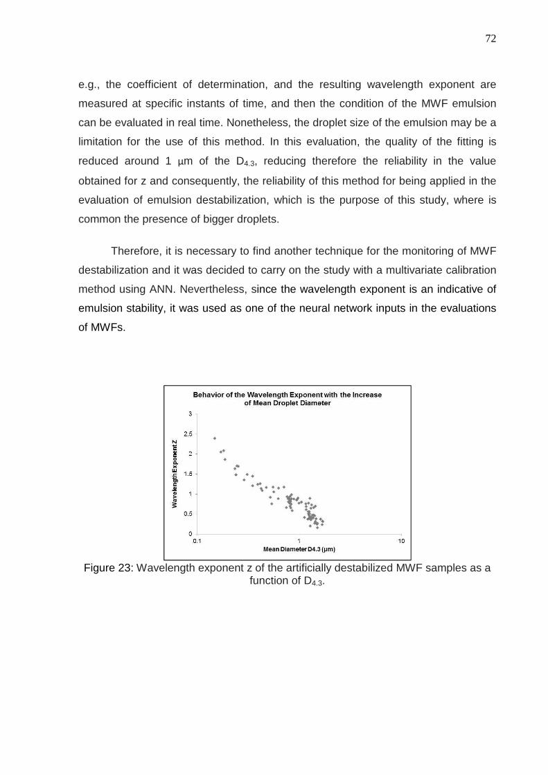
72
e.g., the coefficient of determination, and the resulting wavelength exponent are
measured at specific instants of time, and then the condition of the MWF emulsion
can be evaluated in real time. Nonetheless, the droplet size of the emulsion may be a
limitation for the use of this method. In this evaluation, the quality of the fitting is
reduced around 1 μm of the D4.3, reducing therefore the reliability in the value
obtained for z and consequently, the reliability of this method for being applied in the
evaluation of emulsion destabilization, which is the purpose of this study, where is
common the presence of bigger droplets.
Therefore, it is necessary to find another technique for the monitoring of MWF
destabilization and it was decided to carry on the study with a multivariate calibration
method using ANN. Nevertheless, since the wavelength exponent is an indicative of
emulsion stability, it was used as one of the neural network inputs in the evaluations
of MWFs.
Figure 23: Wavelength exponent z of the artificially destabilized MWF samples as a
function of D4.3.

73
Figure 24: Coefficient of determination R2 for the fitting of Equation 5 to data of the
artificially destabilized MWF samples as a function of D4.3.
5.4. Studies to Estimate the Droplet Size Distribut ion of Rapeseed Oil
Emulsions Based on Neural Network Fitting
As previously shown, the droplet size distribution of an emulsion changes with
the destabilization. Therefore, the aging of an emulsion can be monitored by
monitoring its DSD. For this purpose, it was evaluated the applicability of neural
network models for obtaining DSD of emulsions using the data from the
spectroscopic sensor described in Chapter 4.
The experimental data of rapeseed oil emulsion described in the previous
items were used in the fitting of models to estimate the DSD of these emulsions
based on spectroscopic measurements and fitting of the data by neural networks. As
previously described and illustrated in Figure 12, the experimental data were fitted by
a three-layer feed-forward neural network. Based on preliminary fittings trials, the
following 7 variables were selected as inputs to the model: the measured values of
extinction at the PCA-selected wavelengths (values at 452nm, 662nm e 943nm), the
ultrasound energy transferred to the emulsion during the emulsification process and
the mass fraction of water, oil and emulsifier (i.e., emulsion formulation, previously
described in Chapter 4.1). It was not possible to use only data from spectra to fit an
accurate model for obtaining the DSD of rapeseed oil emulsions due to the high

74
variability of the data, so variables related to emulsion formulation were included as
inputs of the network. All the prepared samples were analyzed after the same time of
preparation (after 5 minutes for absorbance spectrum and after 10 minutes for DSD
analysis); however, most of the samples had presented low emulsion stability,
especially the ones formulated to simulate old emulsions, which caused the high
variability of the measured data. For this reason, it was necessary to add more
information to the network to help in the learning process of the model and the best
result were found using the 7 inputs previously cited. Since in a real application some
of these inputs may not be available, like the inputs related to emulsion formulation, it
is expected that this additional information will not be necessary in the studies of
more stable emulsions and real-case scenario applications. As previously mentioned,
the wavelength exponent z was not included as an input of the ANN due to the
volumetric mean droplet diameter of the samples, with are outside the range of
applicability of this method.
As outputs 20 size classes in the range of 0.03 μm to 20.3 μm were arbitrarily
selected, as multiples of √2, aiming at reconstructing the DSD profile with an
acceptable resolution. This number of size classes as well as its range can be
changed according to the desired applications. In the present study 20 classes in the
mentioned range were considered adequate, in order to compare the results and to
evaluate the technique.
Thus, since the number of inputs and outputs is defined by the specific
characteristics of the system, then the only degree of freedom was the number of
neurons in the hidden layer. In the fitting step, for each value of this number, the
minimum value of the error (Equation 18) was recorded and the best fitting was
obtained with 6 neurons in the hidden layer and 500000 presentations of the data
set.

75
Figure 25: Neural network fitting results for corresponded spectra of rapeseed oil
emulsions, with 7 inputs and 20 outputs (training set).

76
Figure 26: Neural network fitting results for corresponded spectra of rapeseed oil
emulsions, with 7 inputs and 20 outputs (validation set).
Figures 25 and 26 show some results obtained in the best fitting, which are
representative of the whole set. The plots in the left represent the normalized light
extinction spectrum of the emulsion, measured with the spectroscopic sensor. The
graphs in the right represent the corresponding DSD (measured distribution and
distribution calculated by the network), where smaller droplet sizes are representative
of newer emulsions and larger droplet sizes are representative of older emulsions.
Good agreement between calculated and experimental values was obtained for
monomodal as well as for bimodal distributions, indicating the potential of these
models for monitoring oil-in-water emulsions in similar conditions. It is also possible

77
to observe how the measured spectra change with the destabilization of the emulsion
and the growth of the droplet size, proving that they are indeed correlated to each
other. The results of the fitting were presented as DSD curves instead of the more
common “experimental versus calculated” curves because visualization of the results
is better in DSD curves, due to the high number of outputs.
5.5. Studies to Estimate the Droplet Size Parameter s Mean Diameter and
Distribution Variance of Artificially Aged MWF Base d on Neural Network
Fitting
After the evaluation of rapeseed oil emulsions have indicated that the chosen
technique has potential for the monitoring of emulsions, the same method was
applied to artificially aged MWF.
A three-layer feed-forward neural network as illustrated in Figure 12 was fitted
to the experimental data. In total, the following 8 variables were used as inputs: light
extinction values selected by PCA (values at 460nm, 695nm and 943nm),
wavelength exponent, concentration of oil, water and CaCl2, and the time interval
between addition of salt to the emulsion and each measurement (aging time). Once
again, it was not possible to use only data from spectra to fit an accurate model. The
presence of CaCl2 in different concentrations in the emulsions affects the light
absorbance in the measurements. For this reason, it was necessary to compensate
this interference and to add more information to the network to help in the learning
process of the model, being the best result found using the 8 inputs previously cited.
In a real application some of these inputs will not exist (no chemicals are added to
accelerate the emulsion destabilization in real application), so it is expected that this
additional information will not be necessary in the studies of real-case scenario
application.
As outputs of the neural network were selected the volumetric mean diameter
(D4,3) of the droplets (in μm) and variance of the droplet size distribution (in μm2). The
choice of D4.3 as mean diameter was due to its higher sensitivity to the presence of

78
larger particles, which is related to the partial destabilization of the emulsion.
However, it is possible that two populations with different distributions have the same
mean diameter, so the variance of the droplet size distribution was also chosen as an
input to provide information about the dispersivity of the distribution. The best fitting
was obtained with 6 neurons in the hidden layer and 1 million presentations of the
data set to the NN.
Figure 27 shows the results obtained in the fitting for emulsions with different
aging times and consequently different mean diameters and variances. As shown in
the plots, a good agreement between calculated and experimental values was
obtained.
Figure 27: Neural network fitting results for a network with 6 neurons in the hidden
(intermediary) layer.
The evaluation of the relative importance of each input variable of the model
was carried out based on the HIPR method (“Holdback Input Randomization
Method”), proposed by KEMP; ZARADIC and HANSEN ( 2007). The results are

79
shown in Figure 28. According to this analysis, the least important variable is the
wavelength exponent. Thus, this variable was excluded from the inputs and a new
neural network fitting was carried out based on the seven remaining model inputs. As
shown in Figure 29, again there is a good correlation between calculated and
experimental values. Removal of this input has in fact slightly improved the validation
results. No improvement was obtained by removing the other least important inputs,
indicating that this is the best fitted model for this system.
It is surprising that the evaluation of the relative importance of the neural
network inputs has identified the wavelength exponent as the least important variable
in the data set, since this has been a frequently adopted criterion in the literature
associated with emulsion stability. However, since its value is estimated from the
differentiation of spectral data in relation to the wavelength in log-log correlations, it is
possible that, for this data set, the rather low accuracy of such estimation method,
especially for the samples with longer aging times and, consequently, larger
particles, causes too much noise in the data, and that the other variables from the
spectral data (light extinction at 3 different wavelengths) provide similar information
with less noise. This confirms previous findings that the particle size can indeed be a
limitation for the application of the wavelength exponent method, since there are a
significant number of samples in the data set with volumetric mean diameter larger
than 1 μm, i.e., in the size range where it was previously shown to result in a poor
fitting in the calculation of z. In Figure 28 it is also possible to see that the two main
inputs of the model are the concentration of water and oil (MWF), justified by the fact
that they have a direct impact on the droplet population and, consequently, on the
spectroscopic measurements.

80
Figure 28: Relative contribution of each input to the predictive ability of the neural
network model.
Figure 29: Neural network fitting results for a network with 6 neurons in the hidden
(intermediary) layer reducing the number of inputs.

81
5.6. Studies to Rebuild the Droplet Size Distributi on of Artificially Aged MWF
Emulsions Based on Neural Network
Although parameters such as mean diameter and distribution variance can be
used to monitor the aging and stability of emulsions, the droplet size distribution can
provide more complete information about the emulsion structure. Due to that, another
neural network fitting was performed. In this case, 7 variables were used as inputs:
light extinction values selected by PCA at 460nm, 695nm and 943nm, concentration
of oil, water and CaCl2, and the time interval between addition of salt to the emulsion
and each measurement (aging time). In this study the wavelength exponent was not
used because the previous evaluation has shown that it is not so important to the
model.
As outputs of the neural network 17 sizes classes were selected, from 0.04 µm
to 10 µm, as multiples of √2 , aiming at reconstructing the DSD profile with
appropriate resolution. The best fitting was obtained with 6 neurons in the hidden
layer and 500000 presentations of the data set.
Figures 30 and 31 show some of the results obtained in the best fitting, which
are representative of the whole set, for emulsions with different aging times and
consequently different DSD. The plots on the left represent the normalized light
extinction spectrum of the emulsion, measured with the spectroscopic sensor. Those
on the right represent the corresponding DSD (measured distribution and distribution
calculated by the network), where smaller droplet sizes are representative of newer
emulsions and larger droplet sizes are representative of emulsions with higher aging
times. Again the results of the fitting were presented as DSD curves instead of the
more common “experimental versus calculated” curves because visualization of the
results is better in DSD curves, due to the high number of outputs.
A good agreement was obtained between calculated and experimental values,
not only for monomodal but also for bimodal distributions, with different proportions
between each droplet population. It is also possible to observe how the measured
spectra change with the destabilization of the emulsion and the growth of the droplet

82
size, as expected. These results indicate the potential of these models for monitoring
oil-in-water emulsions, although this fitted model is limited to evaluations with similar
conditions and the same set of inputs. It would be interesting to find a model suitable
for a more generic application, even if it is valid in the studied range only. This is
discussed in other parts of this text, in the study of a real-case scenario.
Figure 30: Neural network fitting results for artificially aged MWF, with 7 inputs and
17 outputs (training set).

83
Figure 31: Neural network fitting results for artificially aged MWF, with 7 inputs and
17 outputs (validation set).
5.7. Application of the Neural Network Model to Mon itor MWF Emulsion
Destabilization
The previous model indicates that the combination of a UV/Vis
spectrophotometric system with neural network models results in an optical sensor,
which is capable of detecting changes in DSD during aging of MWF. In order to
evaluate the potential use of this application, a monitoring experiment was carried out
as follows. A commercial metalworking fluid emulsion with concentration of 4 wt.%

84
was artificially destabilized by adding 0.3 wt.% of calcium chloride and the aging was
monitored over time with the optical sensor. These concentrations are within the
range of fitting of the model, thus, of its validity. The spectroscopic data were fed to
the adjusted model in order to estimate the droplet size distribution of the emulsion
and evaluate its change over time.
In Figure 32, the plots on the left represent the normalized light extinction
spectrum of the emulsion, as measured with the spectroscopic sensor, and the plots
on the right represent the corresponding DSD (measured distribution and distribution
calculated by the model). As shown in the plots, the DSD calculated by the model is
similar to the DSD obtained by measuring the samples with the laser diffractometer.
The model was able to calculate the distribution with good accuracy as well as to
detect the evolution of the destabilization of the emulsion, which is associated with
the change in the DSD from monomodal to bimodal. It is also possible to observe the
evolution of the measured spectra with the destabilization of the emulsion and the
growth of the droplet size, so it is clear that both phenomena are correlated.
Although the fitted model is suitable only for applications in similar systems,
the results point out the potential of this technique for monitoring such emulsions,
with the advantage that apparently the results are not affected by multiple scattering,
suggesting that this approach may even be applied to more concentrated emulsions.
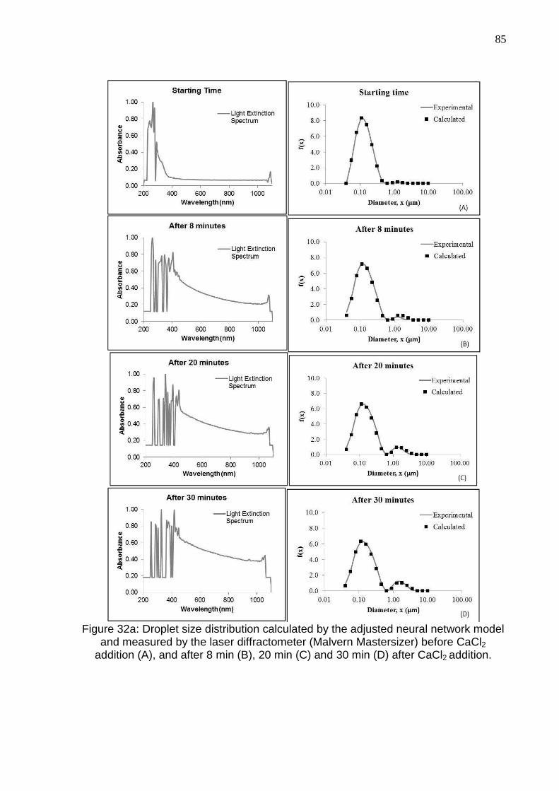
85
Figure 32a: Droplet size distribution calculated by the adjusted neural network model
and measured by the laser diffractometer (Malvern Mastersizer) before CaCl2 addition (A), and after 8 min (B), 20 min (C) and 30 min (D) after CaCl2 addition.

86
Figure 32b: Droplet size distribution calculated by the adjusted neural network model and measured by the laser diffractometer (Malvern Mastersizer) 80 min (E) and 1040
min (F) after CaCl2 addition.
5.8. Application of the Spectroscopic Sensor to the Long-Term Monitoring of
Metalworking Fluids Aging in a Machining Facility
The previous results indicate the potential of this technique for monitoring
emulsion destabilization. However the obtained models are limited to a set of inputs
that may not be available in common applications, like information about emulsion
formulation or addition of chemicals to accelerate the destabilization process. In
order to check the applicability of the method, a long-term monitoring study of
commercial MWFs in a machining facility was carried out. The objective of this
campaign was to obtain information as near as possible of a real-case scenario on
the performance of the spectroscopic probe plus neural network as a sensor for
monitoring MWF destabilization. Data were collected from 7 different commercial
metalworking fluids, during a period of 13 months, from 3 different machines, as
described in Chapter 4.1.2. After cleaning of the raw data set, to eliminate wrong or

87
missing recordings, as well as outliers, the resulting data set contained a total of 88
observations.
The usual control of quality of MWFs consists of periodic analyses of some
properties of the fluid only, and the judgment by the machine operation personnel.
These periodic analyses are the basis for the judgment of the fluid quality by the
machine operation personnel. In this thesis, these results are expressed in the form
of a status classification of the fluid. Thus, in the specific machining facility used in
this study, MWFs are classified as: status 1/green (no signs of deterioration), status
2/yellow (initial signs of deterioration), and status 3/red (high degree of deterioration).
Figure 33 shows the distribution of the collected data of the long-term
monitoring study, grouped by the status in which each sample was classified by the
machine operation personnel. The measured variables in this study, as described in
Chapter 4, are listed below.
• Variables commonly used in the monitoring of MWF quality in the studied
machining facility, whose control is required by specific legislation applied to
machining industry:
• pH;
• Concentration of the fluid, measured in wt.%;
• Nitrite content in the MWF, measured in mg/L;
• Microbiological contamination by ATP method, expressed as log(ATP)
and measured in CFU/mL (colony forming unit per mL).
• Variables from the spectroscopic sensor:
• Wavelength exponent of the samples, z, calculated by the fitting of
Equation 5, where z is the slope of the curve, calculated between 500-
600 nm;
• Linear coefficient of the wavelength exponent fitting, i.e., of the fitting of
Equation 5, which is related to optical properties of the fluid and
emulsion concentration.
• Reference measurements:
• Volumetric mean diameter D4.3, calculated from the obtained DSD,
measured in a Malvern Mastersizer diffractometer.
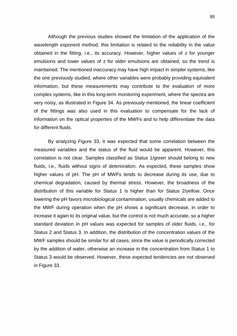
88
Although the previous studies showed the limitation of the application of the
wavelength exponent method, this limitation is related to the reliability in the value
obtained in the fitting, i.e., its accuracy. However, higher values of z for younger
emulsions and lower values of z for older emulsions are obtained, so the trend is
maintained. The mentioned inaccuracy may have high impact in simpler systems, like
the one previously studied, where other variables were probably providing equivalent
information, but these measurements may contribute to the evaluation of more
complex systems, like in this long-term monitoring experiment, where the spectra are
very noisy, as illustrated in Figure 34. As previously mentioned, the linear coefficient
of the fittings was also used in this evaluation to compensate for the lack of
information on the optical properties of the MWFs and to help differentiate the data
for different fluids.
By analyzing Figure 33, it was expected that some correlation between the
measured variables and the status of the fluid would be apparent. However, this
correlation is not clear. Samples classified as Status 1/green should belong to new
fluids, i.e., fluids without signs of deterioration. As expected, these samples show
higher values of pH. The pH of MWFs tends to decrease during its use, due to
chemical degradation, caused by thermal stress. However, the broadness of the
distribution of this variable for Status 1 is higher than for Status 2/yellow. Once
lowering the pH favors microbiological contamination, usually chemicals are added to
the MWF during operation when the pH shows a significant decrease, in order to
increase it again to its original value, but the control is not much accurate, so a higher
standard deviation in pH values was expected for samples of older fluids, i.e., for
Status 2 and Status 3. In addition, the distribution of the concentration values of the
MWF samples should be similar for all cases, since the value is periodically corrected
by the addition of water, otherwise an increase in the concentration from Status 1 to
Status 3 would be observed. However, these expected tendencies are not observed
in Figure 33.

89
Figure 33: Distribution of the variables of the collected data set, grouped by status. (Concentration was measured in %, nitrite in mg/L, microbiological contamination in
CFU/mL and volumetric mean diameter in μm)
9.459.309.159.008.858.70
4.8
3.6
2.4
1.2
0.012108642
0.60
0.45
0.30
0.15
0.00
15129630
0.4
0.3
0.2
0.1
0.076543
0.8
0.6
0.4
0.2
0.0
pH
Fre
que
ncy
Concentration
Nitrite log(ATP)
9.182 0.11839.004 0.078608.983 0.1750
Mean StDevpH
8.014 1.9108.243 0.57747.18 1.489
Mean StDevConcentration
1.309 1.2542.821 0.91754.19 3.549
Mean StDevNitrite
3.988 0.71435.348 0.49046.213 0.5877
Mean StDevlog(ATP)
123
status
Distribution of the Variables of the Collected Data SetGrouped by Status
3.753.002.251.500.750.00
0.8
0.6
0.4
0.2
0.020151050
0.12
0.09
0.06
0.03
0.00
6543210
0.8
0.6
0.4
0.2
0.0
Wavelength Exponent z
Fre
que
ncy
Linear Coefficient of z
D4.3
1.588 0.9082
1.319 0.49981.222 0.5458
Mean StDevWav elength Exponent z
9.824 5.417
8.420 3.0917.814 3.279
Mean StDevLinear Coef f icient of z
0.3787 0.46111.095 1.431
0.8788 0.9686
Mean StDevD4.3
123
status
Distribution of the Variables of the Collected Data SetGrouped by Status

90
Figure 34: Illustration of the obtained spectra of three randomly chosen samples in
the long-term monitoring experiment.
Water-mixed MWFs contain various nutrients for bacteria so that they are
always contaminated with microorganisms. The microbiological contamination is
measured by ATP method, expressed in Figure 33 as log(ATP), and for this variable
some correlation with status is observed. As expected, the log(ATP) increases from
Status 1 to Status 3, since the increase in microbiological contamination favors the
degradation of the fluid. Anaerobic bacteria degrade nitrate or nitrite to ammonia and
sulphate or sulphonate to hydrogen sulphide, causing unpleasant odors, so the
monitoring of nitrite content in the MWFs is also required by specific legislation
applied to machining industry. Fluids with higher nitrite content will present altered
levels of odor, so it was indeed expected to find higher values for this variable in
samples classified as Status 3/red, i.e. with higher signs of deterioration. However,
the corresponding plot in Figure 33 shows no clear tendency regarding this variable.
Although different distribution curves are observed, no clear tendency exists based
on the value of this variable. The analysis of the distribution of the volumetric mean
diameter in Figure 33, used as the reference measurement, does not show any
visual correspondence between the D4.3 and the status, although it is known that the
mean diameter should increase with the aging of the fluid and, consequently, from
Status 1 to Status 3. These results indicate that the MWF monitoring evaluation
adopted by the machine operation personnel is mostly determined by factors related
to microbiological contamination of the fluid, while factors that may affect the
performance of the MWF appear to have less importance. Nevertheless, it was
decided to use of a statistical method to find out if there is a correlation between all
the measured variables and the status classification given by machine operators,
which supposedly should exist.

91
5.8.1. Discriminant Analysis for Evaluating the Sta tus Classification
Assuming that the variables used in monitoring the quality of the MWF (pH,
concentration, nitrite content and microbiological contamination by ATP method) are
adequate for the characterization of the MWF status, these variables were included
in a classification procedure based on the discriminant analysis technique. The
objective in this part of the study is to compare the results obtained with this
statistical technique and the judgment criteria used by the operation personnel in the
machining facility in terms of the three groups: 1/green, 2/yellow and 3/red. The
efficiency of the classification method was based on the fraction of correctly classified
observations in the original groups. Here, the denomination “original group” or
“original status” refers to each of the three groups resulting from the classification
made by the machine operating personnel. Two types of discriminants were tested:
linear and quadratic. Besides the mentioned variables, the wavelength exponent and
the linear coefficient of the linearly adjusted spectra were also included as predictors
in the discriminant analysis. The effect of using only the variables measured by the
spectroscope plus concentration and pH as predictors was also evaluated in these
tests.
Table 3 presents the results obtained with different groups of predictors tested
and the efficiency of each discriminant, indicated as “quality of the fitting”. The
maximum rate of success was 81% and the addition of the wavelength exponent and
the linear coefficient to the group of predictors did not bring any significant
improvement in the quality of the fitting. However, the exclusion of the nitrite content
and microbiological contamination as predictors for the status decreased the quality
of the classification significantly. Since the previous analysis suggests that status
classification done by machine operation personnel may be mostly determined by
factors related to microbiological contamination of the fluid, the effect of using the two
variables related to microbiological contamination as predictors, i.e., nitrite content
and microbiological contamination by ATP method, was evaluated. The maximum
rate of success was 81% in this case, too. Thus, no improvement in the quality of the
fitting was obtained. These results confirm the hypothesis that the variables pH and
concentration do not have much influence on the status classification of the MWF,

92
and also suggest that the factors related to microbiological contamination of the fluid
are not sufficient for determining its quality classification, here represented by the
status.
Table 3: Predictors used for status discrimination and quality of resulting fitting. Fitting 1 Fitting 2 Fitting 3 Fitting 4 Fitting 5 Fitting 6
Predictors
pH pH pH pH pH - Concentration Concentration Concentration Concentration Concentration -
Nitrite Nitrite Nitrite - - Nitrite Log(ATP) Log(ATP) Log(ATP) - - Log(ATP)
- Wavelength Exponent
Wavelength Exponent
Wavelength Exponent
Wavelength Exponent -
- -
Liner Coefficient of Wavelength Exponent
Fitting
-
Liner Coefficient of Wavelength Exponent
Fitting
-
Quality of Linear Fitting 80% 80% 81% 55% 53% 80%
Quality of Quadratic
Fitting 80% 78% 81% 58% 62% 81%
Figures 35 to 40 show the distribution of the data in all fittings. Discriminant
analysis was based on the selected predictors for classifying each observation of the
data set in one of the three groups of status, 1/green, 2/yellow or 3/red, and each
group of this classification is presented in a separated panel of those figures. For
each panel, i.e., each group of classification of the data, the distribution of the original
status of the corresponding set of observations is presented, with the purpose of
analyzing the accuracy of the fitting in each group.
For fittings 1 to 3 (Figures 35 to 37), most of the observations classified as
status 1 or 3, really belong to that group. However, the discriminant analysis was not
able to correctly discriminate the observations that should originally belong to group
2, and observations from all groups were classified in this group. Thus, the
boundaries between these groups of data classification used in the current method of
MWF monitoring are apparently diffuse. For fittings 4 and 5 (Figures 38 and 39) the
results are even worse, with poor quality of fitting observed in all groups. In fitting 6
(Figure 40) most of the observations classified as status 1 or 2, really belong to that
group, so it was the only fitting to improve the results obtained for Status 2. However,
a significant number of observations were misclassified as Status 3.

93
In conclusion, the results of the discriminant analysis show that there is much
overposition of the three groups, which are hardly discriminated by statistical criteria.
This confusion among resulting groups can be caused by one of the following
hypotheses:
• The data were not correctly classified by machine operators and actually
should receive a different status classification. If this hypothesis is true, then a
new method is needed for quality monitoring of MWF.
• The data were correctly classified by machine operators. If this is true, then
there may exist subjective or unmeasured variables besides the currently
measured ones that may have affected the status classification.
Figure 35: Comparison between status distribution of the data after discriminant
analysis and original status in fitting 1.
21
40
30
20
10
0321
12
9
6
3
0
32
20
15
10
5
0
Data classif ied as Status 1
Original Status of the Data
Fre
que
ncy
Data classif ied as Status 2
Data classif ied as Status 3
Distribution of the Data in Fitting 1Linear Fitting

94
Figure 36: Comparison between status distribution of the data after discriminant
analysis and original status in fitting 2.
Figure 37: Comparison between status distribution of the data after discriminant
analysis and original status in fitting 3.
21
40
30
20
10
0321
12
9
6
3
0
32
20
15
10
5
0
Data classif ied as Status 1
Original Status of the Data
Fre
que
ncy
Data classif ied as Status 2
Data classif ied as Status 3
Distribution of the Data in Fitting 2Linear Fitting
21
40
30
20
10
0321
12
9
6
3
0
3
20
15
10
5
0
Data classif ied as Status 1
Original Status of the Data
Fre
que
ncy
Data classif ied as Status 2
Data classif ied as Status 3
Distribution of the Data in Fitting 3Linear Fitting
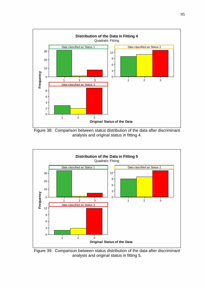
95
Figure 38: Comparison between status distribution of the data after discriminant
analysis and original status in fitting 4.
Figure 39: Comparison between status distribution of the data after discriminant
analysis and original status in fitting 5.
321
30
20
10
0321
12
9
6
3
0
321
8
6
4
2
0
Data classif ied as Status 1
Original Status of the Data
Fre
que
ncy
Data classif ied as Status 2
Data classif ied as Status 3
Distribution of the Data in Fitting 4Quadratic Fitting
321
30
20
10
0321
12
9
6
3
0
321
12
9
6
3
0
Data classif ied as Status 1
Original Status of the Data
Fre
que
ncy
Data classif ied as Status 2
Data classif ied as Status 3
Distribution of the Data in Fitting 5Quadratic Fitting

96
Figure 40: Comparison between status distribution of the data after discriminant
analysis and original status in fitting 6.
These results have motivated the study of an alternative criterion for
classification of these MWF samples, based on the fitting of a neural network model
as a pattern recognition technique, which should be capable of associating a given
pattern of distribution of the input information with the MWF status classes used by
the machine operators. The results are shown in the next item.
5.8.2. Neural Network Fitting for Evaluating Status Classification
In this part of the study, the same groups of predictors used in the previous
evaluation on discriminant analysis were adopted as inputs for the neural network,
having the classification of the MWF status as the output. The input-output
configurations are shown in Table 4. The results are presented in Figures 41 to 45,
as original status versus status calculated by the ANN model, as well as the
distribution of those calculated status, for better showing the overposition between
321
40
30
20
10
0321
10
5
0
32
20
15
10
5
0
Data classif ied as Status 1
Original Status of the Data
Fre
que
ncy
Data classif ied as Status 2
Data classif ied as Status 3
Distribution of the Data in Fitting 6Quadratic Fitting

97
groups. For status 1/green, some of the models were able to calculate values in an
acceptable range, but all results for status 2/yellow and 3/red resulted in poor fittings.
Evaluating the distribution of the calculated data, it is shown that in the training
set the mean of the distribution is close to the expected value for the corresponding
status, although there is overposition between the groups. However, in the validation
set of fittings 1 to 3, the mean values of the distribution of Status 2 are closer to the
value of 3 than the expected value of 2. In fittings 4 and 5, the results are even worse
and the mean values of the distribution of Status 2 are higher than the ones from
Status 3, i.e., it seems to be an inversion between both groups. In fitting 6 it was not
possible to achieve any acceptable result, since all the tested conditions have
returned the value of 0 for all observations and all groups, showing that, in this fitting
and this data set, there are not enough inputs to allow fitting of a model and the only
possible result for the output is that it has the value of 0 in all observations.
Table 4: Inputs used in the neural network fitting.
Neural
Network Fitting 1
Neural Network Fitting 2
Neural Network Fitting 3
Neural Network Fitting 4
Neural Network Fitting 5
Neural Network Fitting 6
Inputs
pH pH pH pH pH - Concentration Concentration Concentration Concentration Concentration -
Nitrite Nitrite Nitrite - - Nitrite Log(ATP) Log(ATP) Log(ATP) - - Log(ATP)
- Wavelength Exponent
Wavelength Exponent
Wavelength Exponent
Wavelength Exponent -
- -
Linear Coefficient of Wavelength Exponent
Fitting
-
Linear Coefficient of Wavelength Exponent
Fitting
-
Outputs Status Status Status Status Status Status
Best Fitting
6 neurons in the hidden layer and 100,000
presentations of the data set
6 neurons in the hidden layer and 100,000
presentations of the data set
6 neurons in the hidden layer and 100,000
presentations of the data set
6 neurons in the hidden layer and 500,000
presentations of the data set
8 neurons in the hidden layer and 500,000
presentations of the data set
It was not possible to achieve any acceptable
result

98
Figure 41: Comparison between calculated status by the neural network model in
fitting 1 and original status of the data.
321
3.0
2.5
2.0
1.5
1.0
0.5
0.0
Status Calculated by the ANN Model
Fre
que
ncy 0.9811 0.1314
2.086 0.50542.857 0.2385
Mean StDev
123
StatusOriginal
Distribution of the Data Calculated by the Neural N etworkGrouped by Original Status of the Data
Training Set
321
2.0
1.5
1.0
0.5
0.0
Status Calculated by the ANN Model
Fre
que
ncy 1.138 0.5001
2.515 0.44002.929 0.1929
Mean StDev
123
StatusOriginal
Distribution of the Data Calculated by the Neural N etworkGrouped by Original Status of the Data
Validation Set

99
Figure 42: Comparison between calculated status by the neural network model in
fitting 2 and original status of the data.
321
2.5
2.0
1.5
1.0
0.5
0.0
Status Calculated by the ANN Model
Fre
que
ncy 0.9814 0.1710
2.099 0.32092.906 0.2354
Mean StDev
123
StatusOriginal
Distribution of the Data Calculated by the Neural N etworkGrouped by Original Status of the Data
Training Set
321
1.6
1.4
1.2
1.0
0.8
0.6
0.4
0.2
0.0
Status Calculated by the ANN Model
Fre
que
ncy 1.246 0.5723
2.748 0.27712.961 0.3098
Mean StDev
123
StatusOriginal
Distribution of the Data Calculated by the Neural N etworkGrouped by Original Status of the Data
Validation Set

100
Figure 43: Comparison between calculated status by the neural network model in
fitting 3 and original status of the data.
321
2.5
2.0
1.5
1.0
0.5
0.0
Status Calculated by the ANN Model
Fre
que
ncy 0.9679 0.1613
2.115 0.29212.905 0.2364
Mean StDev
123
StatusOriginal
Distribution of the Data Calculated by the Neural N etworkGrouped by Original Status of the Data
Training Set
321
1.6
1.4
1.2
1.0
0.8
0.6
0.4
0.2
0.0
Status Calculated by the ANN Model
Fre
que
ncy 1.241 0.6374
2.706 0.34082.973 0.2825
Mean StDev
123
StatusOriginal
Distribution of the Data Calculated by the Neural N etworkGrouped by Original Status of the Data
Validation Set

101
Figure 44: Comparison between calculated status by the neural network model in
fitting 4 and original status of the data.
321
2.5
2.0
1.5
1.0
0.5
0.0
Status Calculated by the ANN Model
Freq
uenc
y 0.9560 0.38182.021 0.17572.784 0.4366
Mean StDev
123
StatusOriginal
Distribution of the Data Calculated by the Neural N etworkGrouped by Original Status of the Data
Training Set
321
35
30
25
20
15
10
5
0
Status Calculated by the ANN Model
Freq
uenc
y 0.7565 0.012962.871 0.65661.870 1.116
Mean StDev
1
23
StatusOriginal
Distribution of the Data Calculated by the Neural N etworkGrouped by Original Status of the Data
Validation Set
43210
0.6
0.5
0.4
0.3
0.2
0.1
0.0
Status Calculated by the ANN Model
Freq
uenc
y
2.871 0.65661.870 1.116
Mean StDev
23
StatusOriginal
Distribution of the Data Calculated by the Neural N etworkGrouped by Original Status of the Data
Validation Set
(Status 1 was excluded for better visualization)

102
Figure 45: Comparison between calculated status by the neural network model in
fitting 5 and original status of the data.
321
1.2
1.0
0.8
0.6
0.4
0.2
0.0
Status Calculated by the ANN Model
Fre
que
ncy 1.025 0.3437
1.854 0.35482.885 0.3402
Mean StDev
123
StatusOriginal
Distribution of the Data Calculated by the Neural N etworkGrouped by Original Status of the Data
Training Set
321
0.9
0.8
0.7
0.6
0.5
0.4
0.3
0.2
0.1
0.0
Status Calculated by the ANN Model
Fre
quen
cy 1.405 1.1932.770 0.45562.195 0.9948
Mean StDev
123
StatusOriginal
Distribution of the Data Calculated by the Neural N etworkGrouped by Original Status of the Data
Validation Set
103
The interpretation of these results lead to hypotheses that are similar to the
ones stated in the previous item, which are:
• The data were not correctly classified by machine operators and actually
should have received a different status classification. If this hypothesis is true,
then a new method is needed for quality monitoring of MWF.
• The data were correctly classified by machine operators. If this is true, then
there may exist subjective or unmeasured variables besides the currently
measured ones that may have affected the status classification.
Therefore, whatever the true hypothesis, the development of a new method for
monitoring the aging of MWF seems necessary.
5.8.3. Coupling of the Spectroscopic Sensor and a N eural Network Model
for the Monitoring of MWF Emulsion Destabilization
The present approach is based on the results obtained with a similar coupling,
as described in item 5.7 of this thesis. Thus, the specific objective in this study is to
use the ability of the neural network model to rebuild the droplet size distribution of
the MWF emulsion from spectroscopic data, and then to adopt the presence of the
population of coalesced droplets as an indicator of destabilization. The appearance
of this second droplet population is shown in Figures 32a and 32b during the process
of artificial destabilization of MWF emulsions.
With this purpose, a three-layer feed-forward neural network like the one
presented in Figure 12 was used to fit the experimental data. A total of 27 variables
were used as inputs: 23 absorbance values selected from 402 nm to 690 nm,
arbitrarily selected in 12 nm intervals – larger intervals did not provide good results,
as well as variables selected by PCA analysis –, MWF concentration, pH, calculated
value for the wavelength exponent and linear coefficient obtained in the linear fitting
used in the calculation of the wavelength exponent. Although the linear coefficient
does not appear to have a physical meaning, apparently it has helped to discriminate

104
the spectra from different fluids. In fact, the optical properties of the fluids would be a
more suitable option, but it was not possible to have access to this information,
especially because these fluids are formulated from a number of substances, and the
formulation itself is not made available by the MWF producers. As previously
mentioned, although the previous studies showed the limitation of the application of
the wavelength exponent method, the decrease of its accuracy with the increase of
droplet size may have high impact in simpler systems, like the one previously
studied, where other variables were probably providing equivalent information, but
these measurements may still contribute to the evaluation of more complex systems,
like in this long-term monitoring experiment, where the spectra are very noisy.
In the present study, data from all fluids and machines were used to fit one
model, only. The outputs of the neural network consisted of 20 sizes classes, from
0.04 µm to 26.7 µm, ordered as multiples of √2. As in the previous fitting (item 5.6),
this number of size classes was arbitrarily adopted in order to reconstruct the DSD of
the samples with an appropriate resolution. The best fitting was obtained with 10
neurons in the hidden layer, after 50000 presentations of the data set to the neural
network.
Figures 46 and 47 show representative results obtained in the fitting and
validation of the model, for samples with different DSD characteristics, which
correspond to different aging times, or status. The graphs at the left show the light
extinction spectra of the MWF emulsions, as measured with the spectroscopic
sensor, and the graphs at the right show the corresponding DSD (measured values
and calculated by the neural network model). These figures show that the differences
in the measured spectra are not clearly observed by visually, possibly due to the
presence of contaminants from the machining process, as well as due to differences
in the optical properties of the different MWFs. However, still it is possible to observe
some evolution of the measured spectra with the destabilization of the emulsion.
In terms of the estimated DSD, good agreement between calculated and
experimental values was obtained for 94% of the samples, for monomodal and
bimodal distributions, and for different proportions of each droplet population. The
rate of success of this fitting was calculated based on the number of observations for

105
which the relative squared error between calculated and observed values were under
1%.
Figure 46: Neural network fitting results for the long-term monitoring study of
commercial MWFs in a machining facility, with 27 inputs and 20 outputs (training set).

106
Figure 47: Neural network fitting results for the long-term monitoring study of
commercial MWFs in a machining facility, with 27 inputs and 20 outputs (validation set).
Representative results for the 6% of the samples for which the model did not
provide the expected result are shown in Figure 48. It is important to mention that in
all the cases showing inaccurate results the model predicted the presence of a
second population of coalesced droplets, which had not been detected in the
measurements. Thus, in all these cases the model provided conservative results, i.e.,
the model associated the information with an aged MWF emulsion.

107
As mentioned in previous parts of this thesis, aging during real machining
operation in a metalworking facility is complex and not easily detected. Besides
microbiological contamination, fluids can be contaminated by solid particles and other
oils in the process, and the MWF concentration can change due to water evaporation
or new dilutions. An additional factor that can affect the results in this case is the
possibly high variability of the collected data, because these data were collected by
different machine operators in industrial scale facilities consisting of different
metalworking equipments, as described. If these factors are taken into consideration,
the resulting fraction of success obtained by the neural network model, i.e., 94% of
the observations, can be considered as a satisfactory result for this system.
As reported in this item of the thesis, the neural network model was able to
predict the presence of the second population of coalesced droplets in the MWF
emulsion samples with a high percentage of success, i.e., for 94% of the
observations. Since the formation of a second population with coalesced droplets,
i.e., consisting of larger droplets, is an indication of emulsion destabilization, it is of
interest that the spectroscopic sensor be able to detect this status in its early steps.
Thus, it is of interest that the sensor plus neural network coupling be as sensitive as
possible to the formation of this second droplet population. A study aimed at this was
carried out, as reported in the next item.
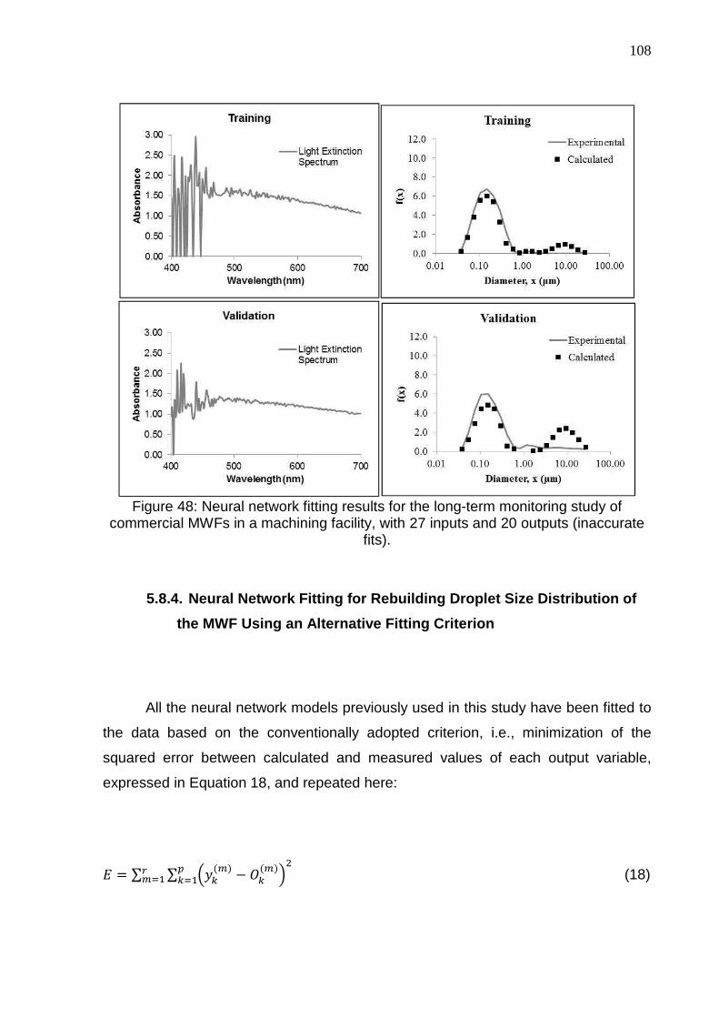
108
Figure 48: Neural network fitting results for the long-term monitoring study of
commercial MWFs in a machining facility, with 27 inputs and 20 outputs (inaccurate fits).
5.8.4. Neural Network Fitting for Rebuilding Drople t Size Distribution of
the MWF Using an Alternative Fitting Criterion
All the neural network models previously used in this study have been fitted to
the data based on the conventionally adopted criterion, i.e., minimization of the
squared error between calculated and measured values of each output variable,
expressed in Equation 18, and repeated here:
G = ∑ ∑ ]̂�B� − Z�̂B� ��̂4�_B4� (18)

109
In order to increase the sensitivity of the neural network model, the criterion for
model fitting was changed in order to increase the importance of the droplet
population formed by coalesced droplets. The squared error in this case is expressed
in the form of Equation 39, where n is the number of size classes used as outputs.
GB�$ = ∑ %>S�&SK − >���K)�'[�04� (39)
In this equation, Acalc is the area under the calculated DSD curve and Aexp is
the area under the experimental DSD curve, expressed by Equations 40 and 41.
>S�&SK = �K:+[�K� S�&S� . ∆�0 (40)
>���K = �K:+[�K� ���� . ∆�0 (41)
In the present study the area under the DSD curve for the coalesced particles
is much larger than the one for the smaller droplets because the size intervals
increase as multiples of √2, and are thus larger for larger droplet sizes. This makes
the squared error (Equation 39) much more sensitive to the formation of coalesced
droplets.
Using this modified network, it was possible to reduce the total number of
inputs to 12 variables: 8 absorbance values arbitrarily selected in 40 nm intervals, in
the range of 402 nm to 690 nm, MWF concentration, pH, calculated value for the
wavelength exponent and linear coefficient obtained in the calculation of the
wavelength exponent. Once more, although the linear coefficient does not have a
physical meaning, apparently it has helped to discriminate data from different fluids
due to the lack of information on the optical properties of the MWF fluids. Data from
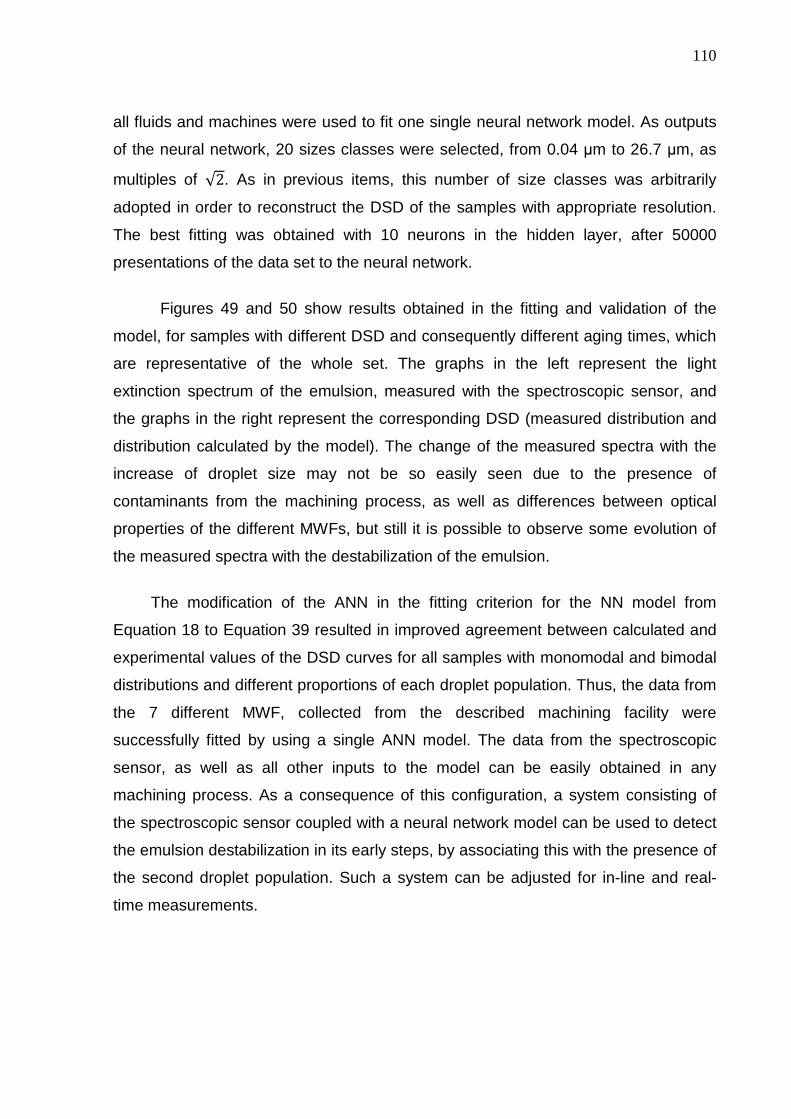
110
all fluids and machines were used to fit one single neural network model. As outputs
of the neural network, 20 sizes classes were selected, from 0.04 µm to 26.7 µm, as
multiples of √2. As in previous items, this number of size classes was arbitrarily
adopted in order to reconstruct the DSD of the samples with appropriate resolution.
The best fitting was obtained with 10 neurons in the hidden layer, after 50000
presentations of the data set to the neural network.
Figures 49 and 50 show results obtained in the fitting and validation of the
model, for samples with different DSD and consequently different aging times, which
are representative of the whole set. The graphs in the left represent the light
extinction spectrum of the emulsion, measured with the spectroscopic sensor, and
the graphs in the right represent the corresponding DSD (measured distribution and
distribution calculated by the model). The change of the measured spectra with the
increase of droplet size may not be so easily seen due to the presence of
contaminants from the machining process, as well as differences between optical
properties of the different MWFs, but still it is possible to observe some evolution of
the measured spectra with the destabilization of the emulsion.
The modification of the ANN in the fitting criterion for the NN model from
Equation 18 to Equation 39 resulted in improved agreement between calculated and
experimental values of the DSD curves for all samples with monomodal and bimodal
distributions and different proportions of each droplet population. Thus, the data from
the 7 different MWF, collected from the described machining facility were
successfully fitted by using a single ANN model. The data from the spectroscopic
sensor, as well as all other inputs to the model can be easily obtained in any
machining process. As a consequence of this configuration, a system consisting of
the spectroscopic sensor coupled with a neural network model can be used to detect
the emulsion destabilization in its early steps, by associating this with the presence of
the second droplet population. Such a system can be adjusted for in-line and real-
time measurements.

111
Figure 49: Neural network fitting results for the long-term monitoring study of
commercial MWFs in a machining facility, using an alternative fitting criterion, with 12 inputs and 20 outputs (training set).

112
Figure 50: Neural network fitting results for the long-term monitoring study of
commercial MWFs in a machining facility, using an alternative fitting criterion, with 12 inputs and 20 outputs (validation set).

113
6. CONCLUSIONS
Monitoring MWFs quality in machining process is critical for the control of
process and product quality, and the conventional methods of quality control in
machining facilities may not be the best alternative to provide the optimal useful life
of these emulsions, with high impact in costs.
Literature suggests that the monitoring of emulsion destabilization could
possibly be used as a better indicator of potential losses in MWFs performance. One
possible method deals with the droplet size distribution, which is directly linked to the
quality and physical stability of an emulsion. Thus, changes in DSD can be used as
an indicator of partial destabilization of an emulsion.
Since changes in the DSD of an emulsion can cause changes in the light
extinction spectra in spectroscopic measurements, one simple method of evaluating
these changes is based on the so called wavelength exponent, z. The applicability of
the wavelength exponent measurement as an indication of the emulsion stability was
investigated in this thesis by monitoring both the turbidity spectra and the DSD of
emulsions over time, for artificially aged MWF samples, as well as by evaluating the
time evolution of the wavelength exponent and the quality of the fitting to the
experimental data.
The results have shown that the wavelength exponent decreases gradually
with the increase in the volumetric mean diameter of the droplets, which is in
agreement with information in the literature. However, the destabilization of the MWF
leads to the formation of a bimodal DSD, resulting in a significant reduction in the
quality of the fitting to the data, expressed by the coefficient of determination, R2,
when the volumetric mean diameter, D4.3, reaches approximately 1µm. The use of
the wavelength exponent has been proposed under the assumption of a monomodal
and monodisperse distribution and the decrease in its value with time has been
associated with the growth in droplet size by coalescence. Thus, the droplet size of
the emulsion may be a limitation for the use of this method, since the reduction in the

114
fitting quality reduces the reliability of the value obtained for z and, consequently, the
reliability of this method in the evaluation of emulsion destabilization.
In this study, an alternative approach is proposed for the monitoring of MWF
destabilization, based on neural network models for obtaining DSD of emulsions
using the data from the spectroscopic sensor. This approach was tested with
rapeseed oil emulsions and with artificially aged MWF. The results based on the
fitting of neural network models showed that the combination of a UV/Vis
spectroscopic system with a neural network results in an optical sensor, which is
capable of detecting changes in the volumetric mean diameter, variance of droplet
size distributions and DSD during aging of commercial MWF, as well as changes in
DSD of rapeseed oil emulsions prepared in laboratory. However, the obtained
models are limited to a set of inputs that may not be available in common
applications; due to the high variability of the data in rapeseed oil emulsions and the
addition of CaCl2 to promote artificial aging of MWF. Nevertheless, these results
pointed out the potential of this technique for monitoring such emulsions, with the
advantage that apparently the results are not affected by multiple scattering,
suggesting that this approach may even be applied to more concentrated emulsions.
In order to check the applicability of this method, a long-term monitoring study
of commercial MWFs in a machining facility was carried out with the objective of
obtaining information on the performance of the spectroscopic probe plus neural
network as a sensor for monitoring MWF destabilization under long-term operation of
machining equipment. In this campaign, the condition of the MWF was classified in
three different categories by operation personnel based on routine analyses and
experience. This classification is the current method of monitoring aging of MWF in
this machining facility; however, a statistical analysis of these data based on
multivariate discriminant analysis indicated that there is much confusion in the
classification results, possibly indicating some failures in the current method of MWF
monitoring. These results have motivated the development of a new method for
monitoring aging of MWF, based on the fitting of a neural network model as a pattern
recognition technique, to rebuild the droplet size distribution of the MWF emulsions
from spectroscopic data, and then to adopt the presence of the population of
coalesced droplets as an indicator of destabilization.

115
The obtained results on the fitting of long-term monitoring data have shown
good agreement between calculated and experimental values for 94% of the
samples, with monomodal and bimodal distributions and different proportions of each
droplet population. This resulting fraction of success obtained by the neural network
model can be considered as a satisfactory result for this system, however, the
formation of a second population with coalesced droplets, i.e., consisting of larger
droplets, is an indication of emulsion destabilization, so it is of interest that the sensor
plus neural network coupling be as sensitive as possible to the formation of this
second droplet population.
For this reason, the program for the fitting of ANN was modified for using a
new criterion for the minimization of the error, considering the differences between
experimental and calculated area under the DSD curve, which is a criterion more
sensitive to the presence of bigger droplets, so it will be more accurate in evaluating
emulsion destabilization. The obtained results on the fitting of long-term monitoring
data with the modified fitting criterion of the ANN resulted in improved agreement
between calculated and experimental values of the DSD curves for all samples with
monomodal and bimodal distributions and different proportions of each droplet
population. Thus, the data from the 7 different MWF, collected from the described
machining facility were successfully fitted by using a single ANN model. The data
from the spectroscopic sensor, as well as all other inputs to the model can be easily
obtained in any machining process. As a consequence of this configuration, a system
consisting of the spectroscopic sensor coupled with a neural network model can be
used to detect the emulsion destabilization in its early steps, by associating this with
the presence of the second droplet population. Such a system can be adjusted for in-
line and real-time measurements, providing a tool for enabling the optimization of
MWF service life. This is a new method for monitoring such emulsions with possible
applications in similar systems, such as pharmaceutical products, emulsion
polymerization processes, crystallization processes, among others.

116
REFERENCES
ABISMAÏL, B. et al. Emulsification by ultrasound: drop size distribution and stability. Ultrasonics sonochemistry , v. 6, n. 1-2, p. 75–83, mar. 1999.
ANGSTRÖM, A. On the Atmospheric Transmission of Sun Radiation II. Geografiska Annaler , v. 12, p. 130–159, 1930.
ASSENHAIMER, C. et al. Use of a spectroscopic sensor to monitor droplet size distribution in emulsions using neural networks. The Canadian Journal of Chemical Engineering , v. 92, n. 2, p. 318–323, 14 fev. 2014.
ASTM D3707. Standard Test Method for Storage Stability of Water -in-Oil Emulsions by the Oven Test PhiladelphiaAmerican Society for Testing and Materials (ASTM), , 2010.
ASTM D3709. Standard Test Method for Stability of Water-in-Oil Emulsions Under Low to Ambient Temperature Cycling Conditions PhiladelphiaAmerican Society for Testing and Materials (ASTM), , 2010.
BENITO, J. M. et al. Formulation, characterization and treatment of metalworking oil-in-water emulsions. Clean Technologies and Environmental Policy , v. 12, p. 31–41, 2010.
BERDNIK, V. V. et al. Characterization of spherical particles using high-order neural networks and scanning flow cytometry. Journal of Quantitative Spectroscopy and Radiative Transfer , v. 102, n. 1, p. 62–72, nov. 2006.
BERDNIK, V. V.; LOIKO, V. A. Particle sizing by multiangle light-scattering data using the high-order neural networks. Journal of Quantitative Spectroscopy and Radiative Transfer , v. 100, n. 1-3, p. 55–63, jul. 2006.
BOHREN, C.F., HUFFMAN, D. . Absorption and scattering of light by small particles . New York: [s.n.].
BRINKSMEIER, E. et al. Current Approaches in Design and Supply of Metalworking Fluids. Tribology Transactions , v. 52, n. 5, p. 591–601, 2009.
BYERS, J. P. Metalworking Fluids . 2. ed. Boca Raton: CRC Press, 2006.
CELIS, M.; GARCIA-RUBIO, L. H. Continuous Spectroscopy Characterization of Emulsions. Journal of Dispersion Science and Technology , v. 23, n. 1, p. 293–299, 2002.
CELIS, M.; GARCIA-RUBIO, L. H. Characterization of Emulsions: A Systematic Spectroscopy Study. Journal of Dispersion Science and Technology , v. 29, n. 1, p. 20–26, jan. 2008.

117
CELIS, M.-T. et al. Spectroscopy measurements for determination of polymer particle size distribution. Colloids and Surfaces A: Physicochemical and Engine ering Aspects , v. 331, n. 1-2, p. 91–96, dez. 2008.
CELIS, M.-T.; GARCIA-RUBIO, L. H. Stability of Emulsions from Multiwavelength Transmission Measurements. Industrial & Engineering Chemistry Research , v. 43, n. 9, p. 2067–2072, abr. 2004.
CHANAMAI, R.; MCCLEMENTS, D. J. Dependence of creaming and rheology of monodisperse oil-in-water emulsions on droplet size and concentration. Colloids and Surfaces A: Physicochemical and Engineering Aspects , v. 172, n. 1-3, p. 79–86, out. 2000.
CHENG, C.; PHIPPS, D.; ALKHADDAR, R. M. Treatment of spent metalworking fluids. Water research , v. 39, n. 17, p. 4051–63, out. 2005.
CHESTNUT, M. H. Confocal microscopy of colloids. Current Opinion in Colloid & Interface Science , v. 2, p. 158–161, 1997.
CHISTYAKOV, B. E. Theory and practical application aspects of surfactants. In: V.B. FAINERMAN, D. M. AND R. M. (Ed.). . Studies in Interface Science . 1st ed. ed.Oxford: Elsevier, 2001. p. 511–618.
COUPLAND, J. N.; JULIAN MCCLEMENTS, D. Droplet size determination in food emulsions: comparison of ultrasonic and light scattering methods. Journal of Food Engineering , v. 50, n. 2, p. 117–120, nov. 2001.
DELUHERY, J.; RAJAGOPALAN, N. A turbidimetric method for the rapid evaluation of MWF emulsion stability. Colloids and Surfaces A: Physicochemical and Engineering Aspects , v. 256, n. 2-3, p. 145–149, abr. 2005.
DICKINSON, E. Interfacial interactions and the stability of oil-in-water emulsions. Pure and Applied Chemistry , v. 64, n. 11, p. 1721–1724, 1992.
DOLL, K. M.; SHARMA, B. K. Emulsification of chemically modified vegetable oils for lubricant use. Journal of Surfactants and Detergents , v. 14, p. 131–138, 2011.
EGGER, H.; MCGRATH, K. M. Aging of oil-in-water emulsions: The role of the oil. Journal of Colloid and Interface Science , v. 299, p. 890–899, 2006.
EL BARADIE, M. A. Cutting Fluids Part 1: Characterisation. Journal of Materials Processing Technology , v. 56, p. 786–797, 1996.
ELICABE, G. E.; GARCIA-RUBIO, L. H. Latex Particle Size Distribution From Turbidimetry Using a Combination of Regularization Techniques. Advances in Chemistry Series , v. 227, p. 83–104, 1990.
GLASSE, B. et al. Turbidimetric Spectroscopy for the Evaluation of Metalworking Fluids Stability. Tribology Transactions , v. 55, n. 2, p. 237–244, mar. 2012.

118
GLASSE, B. et al. Analysis of the Stability of Metal Working Fluid Emulsions by Turbidity Spectra. Chemical Engineering & Technology , v. 36, n. 7, p. 1202–1208, 6 jul. 2013.
GLASSE, B. et al. Turbidimetry for the stability evaluation of emulsions used in machining industry. The Canadian Journal of Chemical Engineering , v. 92, n. 2, p. 324–329, 31 fev. 2014.
GLASSE, B. Monitoring of Metal Working Fluid Emulsion Quality by in-process Light Spectroscopy . [s.l.] Universität Breman, 2015.
GREELEY, M.; RAJAGOPALAN, N. Impact of environmental contaminants on machining properties of metalworking fluids. Tribology International , v. 37, p. 327–332, 2004.
GROSCHE, L. C. Study of the interactions between emulsion flow and a spectrometer probe based on numerical simulations . [s.l.] Universidade de São Paulo, 2014.
GUARDANI, R.; NASCIMENTO, C. A. O. Análise Estatística Multivariada Aplicada a Processos Químicos - Técnicas de Discrim inação e de Classificação de Dados São PauloUniversidade de São Paulo, , 2007.
GUARDANI, R.; NASCIMENTO, C. A. O.; ONIMARU, R. S. Use of neural networks in the analysis of particle size distribution by laser diffraction: tests with different particle systems. Powder Technology , v. 126, n. 1, p. 42–50, jun. 2002.
GUIMARÃES, A. P. et al. Destabilization and Recuperability of Oil Used in the Formulation of Concentrated Emulsions and Cutting Fluids. Chemical and Biochemical Engineering Quarterly , v. 24, n. 1, p. 43–49, 2010.
HARUSAWA, F.; MITSUI, T. Stability of emulsions. Progress in Organic Coatings , 1975.
HASS, R. et al. Optical monitoring of chemical processes in turbid biogenic liquid dispersions by Photon Density Wave spectroscopy. Analytical and Bioanalytical Chemistry , v. online, p. 1–12, 2015.
HAYKIN, S. Neural Networks: A Comprehensive Foundation . 2. ed. New Jersey: Prentice Hall, 1999.
HIEMENZ, P. C.; RAJAGOPALAN, R. Principles of Colloid and Surface Chemistry . Third ed.New York: CRC Press, 1997.
HOLLINGSWORTH, K. G. et al. Fast emulsion droplet sizing using NMR self-diffusion measurements. Journal of Colloid and Interface Science , v. 274, n. 1, p. 244–250, 2004.

119
JOHNS, M. L.; HOLLINGSWORTH, K. G. Characterisation of emulsion systems using NMR and MRI. Progress in Nuclear Magnetic Resonance Spectroscopy , v. 50, n. 2-3, p. 51–70, mar. 2007.
JOHNSON, R. A.; WICHERN, D. W. Applied Multivariate Statistical Analysis . 6th. ed. Upper Saddle River: Prentice-Hall, 2007.
JOLLIFFE, I. T. Principal Component Analysis . New York: Springer, 1986.
JUNG, C. H.; KIM, Y. P. Simplified Analytic Model to Estimate the Ångstrom Exponent in a Junge Aerosol Size Distribution. Environmental Engineering Science , v. 27, n. 9, p. 789–795, 2010.
KEMP, S. J.; ZARADIC, P.; HANSEN, F. An approach for determining relative input parameter importance and significance in artificial neural networks. Ecological Modelling , v. 204, n. 3-4, p. 326–334, jun. 2007.
KIOKIAS, S.; RESZKA, A. A.; BOT, A. The use of static light scattering and pulsed-field gradient NMR to measure droplet sizes in heat-treated acidified protein-stabilised oil-in-water emulsion gels. International Dairy Journal , v. 14, n. 4, p. 287–295, 2004.
KLOCKE, F.; EISENBLÄTTER, G. Dry Cutting. Annals of CIRP , v. 46, n. 2, p. 519–526, 1997.
LAWRENCE, S.; GILES, C. L.; TSOI, A. C. Lessons in neural network training: overfitting may be harder than expected (AAAI Press, Ed.)14th National Conference on Artificial Intelligence. Anais ...Menlo Park: AAAI Press, 1997
MACHADO, A. R.; WALLBANK, J. The effect of extremely low lubricant volumes in machining. Wear, v. 210, n. 1-2, p. 76–82, set. 1997.
MCCLEMENTS, D. J.; COUPLAND, J. N. Theory of droplet size distribution measurements in emulsions using ultrasonic spectroscopy. Colloids and Surfaces A: Physicochemical and Engineering Aspects , v. 117, n. 1-2, p. 161–170, out. 1996.
MIE, G. Beiträge zur Optik trüber Medien, speziell kolloidaler Metallösungen. Annalen der Physik , v. 330, n. 3, p. 377–445, 1908.
MOLLET, H.; GRUBENMANN, A. Formulation Technology: Emulsions, Suspensions, Solid Forms . 1st. ed. Weinheim: Wiley-VCH Verlag GmbH & Co. KGaA, 2001.
MORRISON, I. D.; ROSS, S. Colloidal Dispersions – suspensions, emulsions and foams . 1 edition ed.New York: Wiley-Interscience, 2002.
NASCIMENTO, C. A. O.; GUARDANI, R.; GIULETTI, M. Use of Neural Networks in the Analysis of Particle Size Distribution by Laser Diffraction. Powder Technology , v. 90, p. 89–94, 1997.

120
NOVALES, B. et al. Characterization of emulsions and suspensions by video image analysis. Colloids and Surfaces A: Physicochemical and Engine ering Aspects , v. 221, n. 1-3, p. 81–89, 2003.
OLIVEIRA, J. F. G. DE; ALVES, S. M. Adequação ambiental dos processos usinagem utilizando Produção mais Limpa como estratégia de gestão ambiental. Produção , v. 17, n. 1, p. 129–138, abr. 2007.
REDDY, S. R.; FOGLER, H. S. Emulsion stability: Determination from Turbidity. Journal of colloid and interface science , v. 79, n. 1, p. 101–104, 1981.
RUMMELHART, D., MCCLELLAND, J. Parallel distributed processing explorations in the microstructure of cognition . [s.l: s.n.].
SEINFELD, J. H.; PANDIS, S. N. Atmospheric Chemistry and Physics From Air Pollution to Climate Change . [s.l: s.n.].
SONG, M. et al. Rapid Evaluation of Water-in-Oil (w/o) Emulsion Stability by Turbidity Ratio Measurements. Journal of colloid and interface science , v. 230, n. 1, p. 213–215, 1 out. 2000.
TÁPIA, M. Redes neurais artificiais: uma aplicação na previsã o de preços de ovos . [s.l.] Universidade Federal de Santa Catarina, 2000.
VARGAS, A. K. N. et al. Use of biowaste-derived biosurfactants in production of emulsions for industrial use. Industrial and Engineering Chemistry Research , v. 53, p. 8621–8629, 2014.
VARGAS, A. K. N. Study of emulsion stability using computational flu id dynamics . [s.l.] Universidade de São Paulo, 2014.
VIÉ, R.; JOHANNET, A.; AZÉMA, N. Settling of mineral aqueous suspensions. Classification and stability prediction by neural networks. Colloids and Surfaces A: Physicochemical and Engineering Aspects , v. 459, p. 202–210, 2014.
WILDE, P. J. Interfaces: Their role in foam and emulsion behaviour. Current Opinion in Colloid and Interface Science , v. 5, n. 3-4, p. 176–181, 2000.
ZIMMERMAN, J. B. et al. Design of Hard Water Stable Emulsifier Systems for Petroleum- and Bio-based Semi-synthetic Metalworking Fluids. Environmental Science and Technology , v. 37, n. 23, p. 5278–5288, 2003.

121
APPENDIX A – Publications Resulting from the Presen t Study
1. Papers published in journals
• Use of a spectroscopic sensor to monitor droplet size distribution in emulsions
using neural networks. ASSENHAIMER, C., Machado, L. J., Glasse, B.,
Fritsching, U., Guardani, R.. Canadian Journal of Chemical Engineering, v. 92,
n. 2, p. 318-323, 2014.
• Turbidimetry for the stability evaluation of emulsions used in machining
industry. Glasse, B., ASSENHAIMER, C., Guardani, R. and Fritsching, U.
Canadian Journal of Chemical Engineering, v. 92, n. 2, p. 324-329, 2014.
• Analysis of the stability of metal working fluid emulsion by turbidity spectra.
Glasse, B., Fritsching, U., ASSENHAIMER, C., Guardani, R.. Chemical
Engineering & Technology, v. 36, n. 7, p. 1202-1208, 2013.
2. Oral Presentations
• Use of a Spectroscopic Sensor to Monitor Droplet Size Distribution in
Emulsions Using Neural Networks. ASSENHAIMER, C., Machado, L. J.,
Glasse, B., Fritsching, U., Guardani, R. Emulsification: Modeling,
Technologies and Application, Lyon (France), November, 2012.
• Evaluation of emulsion stability using turbidimetry. Glasse, B., Fritsching, U.,
ASSENHAIMER, C., Guardani, R. Emulsification: Modeling, Technologies and
Application, Lyon (France), November, 2012.
• Use of a Spectroscopic Sensor to Monitor Emulsion Stability Based on
Turbidity Spectra. ASSENHAIMER, C., Glasse, B., Lisboa, J. S., Fritsching,
U., Guardani, R. XIX Congresso Brasileiro de Engenharia Química – COBEQ
2012, Búzios (RJ), September, 2012.
• Uso da Espectroscopia UV-Visível para Estimar a Distribuição de Tamanho de
Gotas em Emulsões Oleosas. ASSENHAIMER, C., Guardani, R., Paiva, J. L.,

122
Glasse, B., Fritsching, U. XXXV Congresso Brasileiro de Sistemas
Particulados - ENEMP 2011, Vassouras (RJ), October, 2011.
3. Poster Presentations
• Avaliação do Tratamento de Efluentes Contendo Resíduos de Fluido de Corte
por Processo UV-H2O2. ASSENHAIMER, C., Seto, L. N., Guardani, R.. XX
Congresso Brasileiro de Engenharia Química – COBEQ 2014. Florianópolis
(SC), October, 2014.
• Estudo da Degradação Térmica de Emulsões de Fluidos de Corte. Postal, V.,
Correia, J., ASSENHAIMER, C., Guardani, R.. Congresso Brasileiro de
Engenharia Química – COBEQ 2014. Florianópolis (SC), October, 2014.
• Estudo Comparativo de Técnicas Numéricas de Inversão para Obtenção de
Distribuição de Tamanho de Gotas em Emulsões. Silva, C. F. B.,
ASSENHAIMER, C., Guardani, R.. Congresso Brasileiro de Engenharia
Química – COBEQ 2014. Florianópolis (SC), October, 2014.

123
APPENDIX B – Exploratory Studies to Estimate the Dr oplet Size Distribution of
Rapeseed Oil Emulsions Based on Optical Models and the Mie Theory
An algorithm based on the model proposed by ELIÇABE and GARCIA-RUBIO
(1990) for estimating droplet size distribution in emulsions, as described in Chapter
3.3.2, was used to rebuild the DSD from spectroscopic measurements. The author
based his model on the optical model (Equation 2, previously presented) and used
regularization techniques and inversion algorithms in data treatment. Based on the
referenced paper, an algorithm was written in Matlab® code and used in this study.
The script was tested with an artificially estimated distribution and with real rapeseed
oil emulsions. For the artificially estimated case, the expected spectra of a droplet
population with normal distribution were calculated by the optical model (Equation 2,
previously presented) and used in the script for evaluation of the rebuilt DSD.
As shown in Figures B.1 and B.2, the calculated distributions do not
correspond to the artificially estimated DSD. This difference may be due difficulties in
implementation of the regularization technique and, for the real emulsion, also due to
multiple scattering effects, not considered in the optical model. Besides, differences
in the optical properties and even numerical limitations of the algorithm can be
responsible for the poor agreement observed.
Although further studies could be done in this approach in order to investigate
the reason for the poor results and to improve them, a different methodology that was
investigated at the same time, based on the association of light scattering spectra
and DSD by multivariate calibration techniques, showed better results. Besides,
Glasse (2015) have intensively studied the application of several inversion methods
for retrieving DSD from the spectroscopic measurements and poor results were
obtained for real emulsions like rapeseed oil emulsion and MWF; only synthetic data
produced good results. In this way, it was decided to focus only in this second
approach, using multivariate calibration techniques, such as neural networks models.
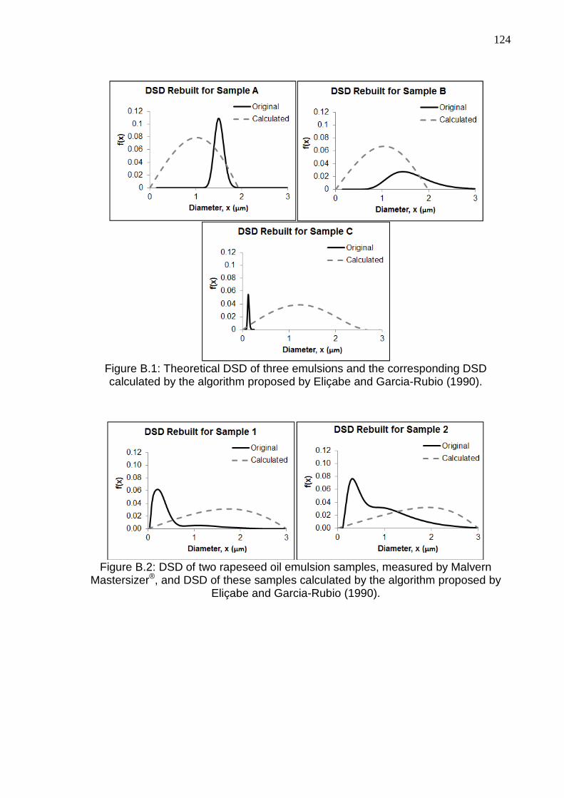
124
Figure B.1: Theoretical DSD of three emulsions and the corresponding DSD calculated by the algorithm proposed by Eliçabe and Garcia-Rubio (1990).
Figure B.2: DSD of two rapeseed oil emulsion samples, measured by Malvern
Mastersizer®, and DSD of these samples calculated by the algorithm proposed by Eliçabe and Garcia-Rubio (1990).

125
APPENDIX C – Algorithm Written in Matlab ® Code Based on the Model
Proposed by Eliçabe and Garcia-Rubio
The following scripts were used in APPENDIX B for droplet size distribution
estimation and are based on the model proposed by Eliçabe and Garcia-Rubio
(1990), described in Chapter 3.3.2.
1. Script for Computation of Mie Efficiencies (used in the described tests for
estimation of droplet size distribution based on li ght scattering models and
inversion techniques)
function result = Mie(m, x) if x==0 result=[0 0 0 0 0 1.5]; elseif x>0 nmax=round(2+x+4*x.^(1/3)); n1=nmax-1; n=(1:nmax);cn=2*n+1; c1n=n.*(n+2)./(n+1); c2n=c n./n./(n+1); x2=x.*x; f=Mie_ab(m,x); anp=(real(f(1,:))); anpp=(imag(f(1,:))); bnp=(real(f(2,:))); bnpp=(imag(f(2,:))); g1(1:4,nmax)=[0; 0; 0; 0]; g1(1,1:n1)=anp(2:nmax); g1(2,1:n1)=anpp(2:nmax); g1(3,1:n1)=bnp(2:nmax); g1(4,1:n1)=bnpp(2:nmax); dn=cn.*(anp+bnp); q=sum(dn); qext=2*q/x2; en=cn.*(anp.*anp+anpp.*anpp+bnp.*bnp+bnpp.*bnpp ); q=sum(en); qsca=2*q/x2; qabs=qext-qsca; fn=(f(1,:)-f(2,:)).*cn; gn=(-1).^n; f(3,:)=fn.*gn; q=sum(f(3,:)); qb=q*q'/x2; asy1=c1n.*(anp.*g1(1,:)+anpp.*g1(2,:)+bnp.*g1(3 ,:)+bnpp.*g1(4,:)); asy2=c2n.*(anp.*bnp+anpp.*bnpp); asy=4/x2*sum(asy1+asy2)/qsca; qratio=qb/qsca; result=[qext qsca qabs qb asy qratio];

126
end ;
2. Script for Computation of Mie Coefficients (used in the last presented
algorithm)
function result = Mie_ab(m,x) z=m.*x; nmax=round(2+x+4*x.^(1/3)); nmx=round(max(nmax,abs(z))+16); n=(1:nmax); nu = (n+0.5); sx=sqrt(0.5*pi*x); px=sx.*besselj(nu,x); p1x=[sin(x), px(1:nmax-1)]; chx=-sx.*bessely(nu,x); ch1x=[cos(x), chx(1:nmax-1)]; gsx=px-i*chx; gs1x=p1x-i*ch1x; dnx(nmx)=0+0i; for j=nmx:-1:2 dnx(j-1)=j./z-1/(dnx(j)+j./z); end ; dn=dnx(n); da=dn./m+n./x; db=m.*dn+n./x; an=(da.*px-p1x)./(da.*gsx-gs1x); bn=(db.*px-p1x)./(db.*gsx-gs1x); result=[an; bn];
3. Script for rebuilding Droplet Size Distribution from Spectroscopic
Measurements
format long clear all clear global clf clc global m turb X I1 I2 Messung_import = xlsread ( 'messung' ); tau= (Messung_import (:,1)); turb=(Messung_import (:,2));

127
wv_up=950; wv_dn=350; tau_2=[]; turb_2=[]; for i=1:(length(tau)) tau_i=tau(i); turb_i=turb(i); if tau_i>wv_dn && tau_i<wv_up tau_2=[tau_2 tau_i]; turb_2=[turb_2 turb_i]; end end tau=reshape(tau_2, length(tau_2),1); turb=reshape(turb_2, length(turb_2),1); if tau(1,1) > tau((length(tau)),1) tau =flipud (tau); turb=flipud(turb); end M=length(tau); n_max= 51; D_min= 5e-9; D_max= 3000e-9; delta_D=(D_max-D_min)/(n_max-1); Vector_D=D_min:delta_D:D_max; Vector_D=transpose (Vector_D); A_ij_vector=[]; for i=1:M tau_i=tau(i,1)*1e-9; lambda=tau_i*1000; im=0.0000001; nm=(1.29+((0.47*(lambda)^2)/((lambda)^2-(0.119) ^2))-((0.08*(lambda)^2)/(2.92^2-(lambda)^2)))^0.5; np=1.45797+0.00598 * (lambda^-2) -0.00036*(lamb da^-4); m=1.35/1.33; for n1=1:1:n_max if n1==1 D_n1=(Vector_D(1,1)); D_n2=(Vector_D(2,1)); D_n3=0; elseif n1==n_max D_n1=(Vector_D((n_max-1),1)); D_n2=(Vector_D(n_max,1)); D_n3=0; else D_n1=(Vector_D(n1,1));

128
D_n2=(Vector_D((n1+1),1)); D_n3=(Vector_D((n1-1),1)); end x_n1=((pi*nm*D_n1)/tau_i); x_n2=((pi*nm*D_n2)/tau_i); x_n3=((pi*nm*D_n3)/tau_i); Mie_maetzler_n1=Mie(m,x_n1); Mie_maetzler_n2=Mie(m,x_n2); Mie_maetzler_n3=Mie(m,x_n3); Q_ext_n1=Mie_maetzler_n1(:,1); Q_ext_n2=Mie_maetzler_n2(:,1); Q_ext_n3=Mie_maetzler_n3(:,1); kernel_n1= pi/4*Q_ext_n1*D_n1^2; kernel_n2= pi/4*Q_ext_n2*D_n2^2; kernel_n3= pi/4*Q_ext_n3*D_n3^2; A1=D_n2*kernel_n1-D_n1*kernel_n2+((kernel_n2-ke rnel_n1)/(2*(D_n2-D_n1)))*((D_n2)^2-(D_n1)^2); A2=0.5*kernel_n1*((D_n2)^2-(D_n1)^2)-(((kernel_ n2-kernel_n1)*D_n1)/(2*(D_n2-D_n1)))*((D_n2)^2-(D_n1)^ 2)+(((kernel_n2-kernel_n1)*((D_n2)^3-(D_n1)^3))/(3*(D_n2-D_n1))); if n1==1 a_ij=(D_n2/delta_D)*A1-(1/delta_D)*A2; A_ij_vector=[A_ij_vector a_ij]; elseif n1==n_max a_ij=(1/delta_D)*A2-(D_n1/delta_D)*A1; A_ij_vector=[A_ij_vector a_ij]; else A3=D_n1*kernel_n3-D_n3*kernel_n1+((kernel_n1-ke rnel_n3)/(2*(D_n1-D_n3)))*((D_n1)^2-(D_n3)^2); A4=0.5*kernel_n3*((D_n1)^2-(D_n3)^2)-(((kernel_ n1-kernel_n3)*D_n3)/(2*(D_n1-D_n3)))*((D_n1)^2-(D_n3)^ 2)+(((kernel_n1-kernel_n3)*((D_n1)^3-(D_n3)^3))/(3*(D_n1-D_n3))); a_ij=(1/delta_D)*A4-(D_n3/delta_D)*A3+(D_n2/del ta_D)*A1-(1/delta_D)*A2; A_ij_vector=[A_ij_vector a_ij]; end end end A_ij_vector=reshape (A_ij_vector, n_max, M); A_ij_vector=A_ij_vector'; A=A_ij_vector; beta=1000; n=n_max; m=M; clear n1 n2 A1 A2 A3 A4 D_n1 D_n2 D_n3 M im np nm lambda delta_D a_ij clear Q_ext_n1 Q_ext_n2 Q_ext_n3 i n_max x_n1 x_n2 x_n3 Mie_maetzler_n1 Mie_maetzler_n2 Mie_maetzler_n3 kernel_n1 kernel_n2 kernel_n3

129
zero_rows = zeros(2,n); zero_matrix = zeros(n-2,2); unit_matrix = eye(n-2,n-2); MATRIX1 = [zero_rows; [zero_matrix unit_matrix] ]; zero_row = zeros(1,n); zero_column = zeros(n-2,1); unit_matrix = eye(n-2,n-2); MATRIX2 = [zero_row ; [zero_column unit_matrix zero_column] ; zero_row]; zero_rows = zeros(2,n-2); zero_columns = zeros(n,2); MATRIX3 = [[unit_matrix; zero_rows] zero_column s]; MATRIX4 = toeplitz([[0 -2] zeros(1,n-2)]); MATRIX4(n,:)=zeros(1,n); MATRIX4(:,n)=zeros(n,1); MATRIX5 = toeplitz([[0 -2] zeros(1,n-2)]); MATRIX5(1,:)=zeros(1,n); MATRIX5(:,1)=zeros(n,1); MATRIX6=toeplitz([0 0 1 zeros(1,n-3)]); H = MATRIX1 + 4*MATRIX2 + MATRIX3 + MATRIX4 + MATRI X5 + MATRIX6; BETA_MATRIX = [beta^2 zeros(1,n-1); zeros(n-2,n); z eros(1,n-1) beta^2]; FINAL_MATRIX = BETA_MATRIX + H; [K,p]=chol(FINAL_MATRIX); X=A*K^(-1); clear zero_column zero_columns zero_matrix zero_row zero_rows unit_matrix options tau_i p MATRIX1 MATRIX2 MATRIX3 MATRIX4 MATRIX5 MATRIX6 gamma_amount=1000; gamma_min=-35; gamma_max=-5; gamma_chain=logspace(gamma_min,gamma_max,gamma_amou nt); V_gamma_vec=[]; I1=eye(n); I2=eye(m); for i=1:gamma_amount gamma=gamma_chain (1,i); V_gamma=( m*(((norm((I2-((X*((transpose(X)*X + gamma.*I1)^-1)*transpose(X))))*turb))^2)/((trace(I2-((X*((trans pose(X)*X + gamma*I1)^-1)*transpose(X)))))^2))); V_gamma_vec=[V_gamma_vec V_gamma]; end [V_gamma_value V_index]=min(V_gamma_vec); gamma_opt=gamma_chain(V_index);

130
f = ((transpose (A))*A+gamma_opt*FINAL_MATRIX)^-1*( transpose(A))*turb; Vector_D_plot=Vector_D*10^9; f_plot=f/sum(f); hold all xlabel( 'Droplet Size in nm' ); ylabel( 'normalized f(D)' ); semilogx(Vector_D_plot,f_plot); hold off