1

Volume 20, Number 1 – March 2018 C h i n a A c c o u n t i n g a n d F i n a n c e R e v i e w

中 国 会 计 与 财 务 研 究

2018 年 3 月 第 20 卷 第 1 期

Corporate Environmental Performance, Accounting Conservatism, and Stock Price Crash Risk: Evidence from China * Xingqiang Du 1 Received 16th of August 2017 Accepted 19th of January 2018 © The Author(s) 2018. This article is published with open access by The Hong Kong Polytechnic University

Abstract Using a sample of 8,173 firm-year observations from the Chinese stock market during the

period 2009–14, this study examines the influence of corporate environmental performance

on stock price crash risk and further investigates the moderating effect of accounting

conservatism. Specifically, based on hand-collected data on environmental performance, the

findings show that corporate environmental performance is significantly negatively related

to future crash risk, suggesting that environmentally friendly firms face less future crash risk.

Moreover, accounting conservatism weakens the negative relationship between corporate

environmental performance and future crash risk. These results are robust to different

measures of stock price crash risk and corporate environmental performance, and remain

valid after controlling for the potential endogeneity between corporate environmental

performance and stock price crash risk.

Keywords: Corporate Environmental Performance, Stock Price Crash Risk, Accounting

Conservatism, China

* I deeply appreciate the constructive comments and informative guidance from Prof. Gang Hu (the Editor)

and the anonymous reviewer, as well as the many valuable suggestions received from Quan Zeng, Hongmei Pei, and Yingying Chang. Especially, I must offer my thanks to Quan Zeng for his excellent research assistance for this study. I acknowledge the financial support of the Key Project of Key Research Institute of Humanities and Social Science in Ministry of Education (approval number: 16JJD790032), the National Natural Science Foundation of China (approval number: NSFC-71572162), and the Training Program of Fujian Excellent Talents in University (FETU).

1 Correspondence: Xingqiang Du, Accounting Department, School of Management, Xiamen University, 422 Siming South Road, Xiamen, Fujian, China (361005). Email: xqdu@xmu.edu.cn.

2

公司环境绩效、会计稳健性与股价崩盘风险*

杜兴强2

   摘要

基于中国资本市场 2009 至 2014 年期间 8,173 个公司-年观测值的样本，本文研究

了公司环境绩效对股价崩盘风险的影响，进而分析了会计稳健性的调节效应。基于手

工搜集的公司环境绩效数据，本文发现公司环境绩效与未来的股价崩盘风险显著负相

关，说明环境友好型的企业经历了较低的未来股价崩盘风险。此外，会计稳健性弱化

了公司环境绩效对股价崩盘风险的抑制效应。进一步，采纳一系列其他度量股价崩盘

风险与环境绩效的变量并不改变本文的主要发现。最后，本文发现在控制了公司环境

绩效与股价崩盘风险之间的内生性后上述研究发现依然成立。

关键词：公司环境绩效、股价崩盘风险、会计稳健性、中国

* 作者感谢胡罡教授（执行编辑）与匿名审稿人的宝贵意见，曾泉、裴红梅和常莹莹有益的建议，

以及曾泉的研究助手工作。作者致谢教育部人文社科基地重大项目（16JJD790032）与国家自然科

学基金（71572162）的资助。 2 杜兴强，厦门大学管理学院会计系教授、博士生导师；Email：xqdu@xmu.edu.cn。

Corporate Environmental Performance and Stock Price Crash Risk 3

I. Introduction

In recent years, many studies have focused on corporate environmental performance

(responsibility) to examine its determinants and economic consequences. Cormier et al.

(2004), Du et al. (2014), Meng et al. (2013), Paillé et al. (2014), and Walker et al. (2013)

investigate the effects of ecological environment, regulatory pressure, top management team

turnover, human resource policies, and religion on corporate environmental performance.

Cai and He (2014), Cohen et al. (1997), Dixon-Fowler et al. (2013), Du (2015a), and

Guenster et al. (2010) examine the impacts of environmental performance on cumulative

abnormal returns, operating efficiency, stock returns, and equity prices. Nevertheless, the

literature provides insufficient evidence on how the market reacts to corporate

environmental performance. In response to this gap, the present study examines the

relationship between corporate environmental performance and stock price crash risk.

Studies have found that firms with better environmental performance have

higher-quality financial reporting (Du et al., 2017; Ingram and Frazier, 1980; Orlitzky et al.,

2003) and engage in fewer bad news hoarding activities (Du et al., 2017). Therefore, this

study predicts that corporate environmental performance is significantly negatively

associated with stock price crash risk. In addition, Petersen (2004) and Petersen and Rajan

(1994) find that hard information (e.g. financial information) and soft information (e.g.

voluntary environmental information disclosure) interact with each other (substitute or

strengthen). This study predicts that accounting conservatism attenuates the mitigating effect

of environmental performance on stock price crash risk.

This study is focused on the Chinese context for two reasons. First, China’s rapid

economic development has been accompanied by very serious environmental pollution (Du,

2015b). Second, Siegel and Vitaliano (2007) and Zyglidopoulos et al. (2012) argue that

corporate environmental performance is inclined to bring out negative externalities for

stakeholders. In addition, Zyglidopoulos et al. (2012) find that firms would rather improve

their strengths related to corporate social responsibility (CSR), such as corporate

philanthropy, than mitigate their CSR weaknesses, such as environmental pollution. Du

(2015b) finds that there is an inherent inconsistency between different CSR dimensions and

further documents that corporate philanthropy is habitually used by some firms to offset the

negative image created by environmental wrongdoing. These findings, taken together,

suggest that CSR-based conclusions may not fit well with corporate environmental

performance, especially in emerging markets such as China, where environmental

consciousness and business ethics are still far from optimal.

For empirical tests, I hand-collect data on corporate environmental performance and

construct a sample of 8,173 firm-year observations from the Chinese stock market during

the period 2009–14. Using this sample, this study examines the influence of corporate

environmental performance on stock price crash risk, and further investigates the

4 Du

moderating effect of accounting conservatism. In brief, my findings reveal several things.

First, corporate environmental performance is significantly negatively associated with stock

price crash risk, suggesting that environmentally friendly firms experience less future crash

risk. Second, accounting conservatism attenuates the negative relationship between

corporate environmental performance and future crash risk. Third, my findings are robust to

different measures of crash risk and corporate environmental performance. Finally, my

findings are valid after controlling for the endogeneity between corporate environmental

performance and future crash risk.

This study contributes to the literature in several ways. First, to the best of my

knowledge, this is one of few, if not the first, to investigate empirically the association

between corporate environmental performance and stock price crash risk. In recent years, a

branch of the existing literature has examined the influence of CSR or corporate

philanthropy on stock price crash risk (Kim et al., 2014; Zhang et al., 2016). However, as

Chen et al. (2008), Du (2015b), and Koehn and Ueng (2010) argue, different dimensions of

CSR may be inherently inconsistent. For example, some corporations may use corporate

philanthropy to cover their environmentally unfriendly behaviour, low product quality, or

poor employee relations (Du, 2015b). Therefore, one can question whether different CSR

dimensions similarly or asymmetrically affect stock price crash risk. Using the context of

China, this study aims to fill the above gap in the literature by examining whether corporate

environmental performance impacts future crash risk.

Second, extending Kim and Zhang’s (2016) examination of the effect of accounting

conservatism on stock price crash risk, I investigate the moderating effect of accounting

conservatism on the association between environmental performance and stock price crash

risk. Theoretically, accounting conservatism suggests that managers present a lower level of

bad news hoarding, which negatively impacts stock price crash risk. Then, referring to

Petersen (2004) and Petersen and Rajan (1994), accounting conservatism, as “hard

information”, and environmental performance, as “soft information”,3 substitute for each

other in mitigating future crash risk. My findings validate the notion that accounting

conservatism attenuates the negative association between corporate environmental

performance and future crash risk.

Third, this study adopts multiple measures of stock price crash risk to provide more

convincing findings regarding the mitigating effect of corporate environmental performance

on future crash risk. Specifically, this study employs four measures of stock price crash risk

(two for main tests and two for robustness checks), including a dummy variable for whether

3 It is Petersen (2004) who classifies information into hard information and soft information. According to

Petersen (2004), hard information is more likely to be transmitted, processed, and reduced to numbers. In addition, information that is difficult to summarise completely as a numeric score is called soft information. As such, financial information provided in a firm’s financial statements can be classified as hard information due to its numeric nature, while corporate environmental performance is soft information because of its scattered nature in non-financial information in notes or CSR reports.

Corporate Environmental Performance and Stock Price Crash Risk 5

a firm-year’s stock price experiences one or more crash risks (CRASH3.09), the negative

skewness of firm-specific weekly returns (NCSKEW), an ordered variable to capture the

number of stock price crashes experienced by a firm (CRASHN3.09), and the asymmetric

volatility between negative and positive firm-specific weekly returns (DUVOL) (i.e. the

down-to-up volatility of the likelihood of future stock price crash risk).

Finally, using the context of China, the largest emerging market and second largest

economy in the world, this study adds to the literature on the relationship between specific

CSR dimensions (environmental performance) and corporate financial behaviour. The

majority of the literature focuses on developed markets in which mature business ethics and

governance mechanisms bring out stronger pressures motivating firms to fulfil their

environmental responsibilities (Sharfman and Fernando, 2008). However, conclusions based

on developed markets may not be a good fit with emerging markets such as China, where

business ethics are immature, corporate governance is incomplete, and environmental

consciousness is weak. As a result, it is necessary for researchers to examine separately the

influence of environmental performance on corporate financial behaviour, such as stock

price crash risk, in emerging markets. It is expected that the findings relating to emerging

markets will provide important supplementary evidence to those regarding developed

markets.

The second section reviews the literature and develops the research hypotheses. The

third section introduces the empirical models and variables. In the fourth section, I report the

sample, data, and descriptive statistics. The fifth section reports main findings; the sixth

section conducts a variety of robustness checks, and the seventh section discusses potential

endogeneity. The final section summarises the conclusions.

II. Literature Review and Hypotheses Development

2.1 Literature Review

Prior studies have examined whether tax sheltering, accounting conservatism, and

opaque financial reporting affect future crash risk (Chen et al., 2001; Hutton et al., 2009;

Kim et al., 2011; Kim et al., 2012; Kim and Zhang, 2016). In recent years, a growing branch

of research has addressed the association between CSR and corporate financial behaviour,

including crash risk (Cui et al., 2015; Deng et al., 2013; El Ghoul et al., 2011; Kim et al.,

2014). However, findings regarding the effect of CSR on stock price crash risk may not be

applied directly to specific CSR dimensions because different CSR dimensions may be

inherently inconsistent (Chen et al., 2008; Du, 2015b; Koehn and Ueng, 2010). Moreover,

Zyglidopoulos et al. (2012) suggest that researchers should differentiate CSR strengths from

CSR weaknesses because firms may increase CSR strengths, such as corporate philanthropy,

rather than reducing CSR weaknesses, such as corporate environmental pollution. CSR

strengths refer to “the additional benefits beyond those required by law and narrow

6 Du

economic interest that a firm provides to its stakeholders”, and CSR weaknesses refer to

“the negative effects that a firm’s operation has on its stakeholders that remain after a firm’s

CSR activities” (Zyglidopoulos et al., 2012). As a result, conclusions about the association

between CSR (corporate philanthropy) and crash risk may not fit corporate environmental

performance. In this context, extant research provides little evidence on the impact of ethical

factors embedded in corporate environmental performance on stock price crash risk (Giuli

and Kostovetsky, 2014). This study fills the above gaps and contributes to the literature by

examining the impact of corporate environmental performance on stock price crash risk.

2.2 The Influence of Corporate Environmental Performance on Stock Price

Crash Risk

Environmental concerns have become increasingly prominent in China, because many

Chinese enterprises always greedily pursue profit at the cost of environmental destruction

(Du, 2015b). Environmental efforts may be expensive, but environmentally responsible

firms are likely to build a good reputation through environmental protection (Konar and

Cohen, 2001; Murphy, 2002). Due to their good reputation, environmentally friendly firms

can obtain support from stakeholders (Russo and Fouts, 1997), which is beneficial to their

legitimacy and provides competitive advantages. For example, Heyes (1996) finds that

lenders value environmental risk, applaud environmentally responsible firms, and charge

environmentally friendly firms lower rates of interest.4 Thus, environmental performance is

negatively related to future operational uncertainty, which results in lower future crash risk.

In addition, environmentally responsible firms face lower litigation risk. In a firm’s

financial statements, corporate environmental responsibility is classified as contingent

liabilities (Keiso et al., 2007). When enterprises fail to take effective measures to control

their pollution or environmentally unfriendly activities, they may be statutorily compelled to

discontinue their operations (they may even go bankrupt). Environmentally responsible

firms convey signals of lower environmental uncertainty—which is associated with lower

likelihood of operational discontinuity and distress—to the market, resulting in lower

information uncertainty. For example, Toms (2002) finds that firms with advanced

environmental management systems can effectively signal to the market that they face

significantly lower systemic risk. To sum up, environmentally friendly firms are less likely

to experience future crash risk than firms with poor environmental performance.

Furthermore, it is very difficult for investors to assess the reliability of accounting

numbers. It is found that environmentally friendly firms have better financial performance

4 I also provide some supporting evidence. The China Banking Regulatory Commission (CBRC)

statutorily requires commercial banks to consider corporate environmental performance as one of the crucial lending criteria. Moreover, central and local governments mandatorily require Chinese enterprises to take corporate environmental responsibility, and urge commercial banks to charge a higher interest rate on debts to environmentally unfriendly firms, and even legitimately prohibit banks from lending to heavily polluting firms.

Corporate Environmental Performance and Stock Price Crash Risk 7

(Du et al., 2017; Ingram and Frazier, 1980; Orlitzky et al., 2003), are more likely to

maintain a higher level of financial reporting quality, and are less likely to engage in bad

news hoarding (Du et al., 2017). Moreover, to confirm the validity of financial information,

stakeholders must collect “soft information” from other sources of information to judge

whether managers are honest and financial reporting is credible (Beaulieu, 2001). In this

regard, voluntary environmental information disclosure (environmental performance) can

serve as a conduit by which investors obtain incremental information to judge whether

managers can be trusted and financial information can be believed. For example, it has been

found that socially responsible firms are less likely to engage in unethical activities. Kim et

al. (2012) show that socially responsible firms place tighter constraints on earnings

management. Lanis and Richardson (2012) find a negative association between CSR activity

and tax aggressiveness, a socially irresponsible and illegitimate activity. In a nutshell, if

stakeholders ensure managers’ moral integrity through environmental performance, they

may believe managers to be less likely to hoard bad news, and thus believe that

environmentally responsible firms are less at risk of crash in the future.

Finally, environmentally friendly firms disclose more (voluntary) non-financial

information to upgrade information transparency (Dhaliwal et al., 2011). Therefore, firms

with good environmental performance always attract more analyst coverage and experience

fewer analyst forecast errors (Dhaliwal et al., 2011; 2012). As a result, information

asymmetry between investors and managers is mitigated, and thus managers are less likely

to conceal bad news. Investors can also use incremental non-financial information provided

by environmentally friendly firms to determine the ethical honesty of managers. The above

arguments, taken together, suggest that environmentally friendly firms engage in less bad

news hoarding and thus are less likely to experience future crash risk.

Overall, environmentally responsible firms can obtain good reputation and competitive

advantage, increase (reduce) the likelihood of going concern (discontinuity), convince

investors of managers’ moral integrity, improve information transparency, and indicate

managers’ lower likelihood of hoarding bad news. Ultimately, environmentally friendly

firms have lower future crash risk. Based on the above discussion, Hypothesis 1 is proposed

as follows:

Hypothesis 1: Ceteris paribus, corporate environmental performance is negatively

associated with future crash risk.

2.3 The Moderating Effect of Accounting Conservatism

Managers exploit information asymmetry, utilising information advantage over

investors to engage in opportunistic behaviour and hoard bad news (Kim et al., 2011), which

brings out future crash risk. However, accounting conservatism mitigates the extent of

managers’ bad news hoarding behaviour and reduces future crash risk (Kim and Zhang,

8 Du

2016). In response, I further address the moderating effect of accounting conservatism on

the negative relationship between corporate environmental performance and future crash

risk. According to Petersen (2004), information can be partitioned into hard and soft

information. Hard information is numeric in nature and can be transmitted and processed

(Petersen, 2004). Accounting conservatism is calculated using data from financial

statements and the market, and should be classified as “hard information” because of its

numeric nature. However, it is difficult for investors to summarise environmental

performance numerically, so corporate environmental performance should be classified as

soft information.

According to Petersen (2004), hard and soft information can be substituted for each

other in the lending market, although soft information may be hard in some cases. Petersen

and Rajan (1994) find that firms can successfully negotiate a lower interest rate through

communicating soft information to banks. Analogically, environmental performance as soft

information and accounting conservatism as hard information interactively affect a firm’s

hoarding of bad news and impact stock price crash risk. Previous studies (e.g. Costello and

Wittenberg-Moerman, 2011; Dhaliwal et al., 2011; Petersen and Rajan, 1994) have reported

the substitutive effect between hard information in a firm’s financial statement and soft

information on corporate behaviour. Based on the literature, I predict that the negative

association between corporate environmental performance and stock price crash risk is less

pronounced for firms with higher conservatism scores than for those with lower

conservatism scores. Based on the above discussion, I formulate Hypothesis 2 in the

alternative form as follows:

Hypothesis 2: Ceteris paribus, accounting conservatism attenuates the negative

association between corporate environmental performance and future crash risk.

III. Empirical Model Specification and Variables

3.1 Multivariate Test Model for Hypothesis 1

To test Hypothesis 1, which predicts that corporate environmental performance is

negatively associated with future stock price, I estimate Eq. (1) to link future crash risk with

corporate environmental performance and firm-specific control variables (Hutton et al.,

2009; Kim et al., 2011):

CRASHt=α0+α1CEPt-1+α2BLOCK t-1+α3NCSKEWt-1+α4INST_SHRt-1+α5ANALYSTt-1

+α6DTURNt-1+α7SIGMAt-1+α8RETt-1+α9SIZEt-1+α10DTEt-1+α11BTMt-1

+α12ROAt-1+α13ACCMt-1+α14TAXt-1+α15PENALTYt-1+α16STATEt-1

+Industry Dummies+Year Dummies+ε (1)

Corporate Environmental Performance and Stock Price Crash Risk 9

In Eq. (1), the dependent variable is stock price crash risk, labelled CRASH. In the

main tests, this study employs NCSKEW and CRASH3.09 to measure stock price crash risk.

NCSKEW is the negative skewness of firm-specific weekly returns. CRASH3.09 is a dummy

variable equal to 1 if a firm-year’s stock price experiences one or more crashes and 0

otherwise (Hutton et al., 2009; Kim et al., 2011). The independent variable is corporate

environmental performance, labelled CEP. In Eq. (1), the negative, significant coefficient on

CEP (α1) is consistent with Hypothesis 1.

Following the literature (Chen et al., 2001; Hutton et al., 2009; Kim et al., 2011), I

include a set of control variables in Eq. (1). First, this study refers to Kim et al. (2011) and

includes several variables concerning governance mechanism (i.e. BLOCKt-1, INST_SHRt-1,

ANALYSTt-1) into Eq. (1). BLOCKt-1 is the percentage of shares held by the controlling

shareholder in year t-1, INST_SHRt-1 is the percentage of shares owned by institutional

investors in year t-1 (Kim et al., 2011), and ANALYSTt-1 is the natural logarithm of (1+ the

number of analyst coverage) in year t-1 (Kim et al., 2011; Chen et al., 2001).

Second, in Eq. (1), I include NCSKEWt-1, DTURNt-1, SIGMAt-1, RETt-1, SIZEt-1, DTEt-1,

BTMt-1, ROAt-1, and ACCMt-1, which are taken from Kim et al. (2011) and Chen et al. (2001).

NCSKEWt-1 is the negative skewness of firm-specific weekly returns in year t-1. DTURNt-1

is the average monthly share turnover over the current calendar year period minus the

average monthly share turnover over the previous calendar year period (where monthly

share turnover is calculated as the monthly trading volume divided by the total number of

shares outstanding during the month) (Kim et al., 2011; Chen et al., 2001). SIGMAt-1 is the

standard deviation of firm-specific weekly returns over the calendar year period t-1

(multiplied by 100) (Kim et al., 2011). RETt-1 denotes the arithmetic average of

firm-specific weekly returns in year t-1 (multiplied by 100) (Kim et al., 2011). SIZEt-1 is the

natural logarithm of the market value of equity at the end of year t-1 (Kim et al., 2011;

Hutton et al., 2009). DTEt-1 is the ratio of total liabilities at the end of year t-1 to the market

value of equity at the end of year t-1. BTMt-1 is the lagged ratio of book-to-market, measured

as the book value scaled by the market value of equity at the end of year t-1 (Chen et al.,

2001; Hutton et al., 2009). ROAt-1 is return on total assets in year t-1, measured as income

before extraordinary items divided by lagged total assets (Kim et al., 2011). ACCMt-1

denotes discretional accruals, measured as a three-year moving sum of the absolute value of

discretionary accruals based on the modified Jones model (Hutton et al., 2009).

Third, Kim et al. (2011) find that tax avoidance is positively related to future crash risk,

and thus I include a firm’s estimated likelihood of tax sheltering (TAXt-1) (Kim et al., 2011).

Fourth, Eq. (1) includes PENALTYt-1 to isolate the influence of managers’ moral

integrity on environmentally friendly activities. PENALTYt-1 is a dummy variable, equal to 1

if a firm is punished by regulators for financial misconduct and 0 otherwise.

Fifth, Eq. (1) includes STATEt-1, a dummy variable equal to 1 when the ultimate

10 Du

controlling shareholder of a listed firm is a (central or local) government agency or

government-controlled enterprise in year t-1 and 0 otherwise.

Finally, a set of year and industry dummy variables are incorporated into Eq. (1) to

control for the year and industry fixed effects. Please refer to Appendix 1 for variable

definitions.

3.2 Multivariate Test Model for Hypothesis 2

Hypothesis 2 predicts that accounting conservatism attenuates the negative association

between environmental performance and future crash risk. To test Hypothesis 2, I estimate

Eq. (2) to link future crash risk (CRASH) with environmental performance (CEP),

accounting conservatism (C_SCORE), the interactive item (CEP×C_SCORE), and a set of

firm-specific control variables:

CRASHt=β0+β1CEPt-1+β2C_SCOREt-1+β3CEPt-1×C_SCOREt-1+β4BLOCKt-1

+β5NCSKEWt-1+β6INST_SHRt-1+β7ANALYSTt-1+β8DTURNt-1

+β9SIGMAt-1+β10RETt-1+β11SIZEt-1+β12DTEt-1+β13BTMt-1

+β14ROAt-1+β15ACCMt-1+β16TAXt-1+β17PENALTYt-1

+β18STATEt-1+Industry Dummies+Year Dummies+δ (2)

In Eq. (2), the dependent and independent variables are still stock price crash risk

(CRASHt) and corporate environmental performance (CEPt-1), respectively. The moderating

variable is accounting conservatism score (C_SCOREt-1). My major concern in Eq. (2) is the

interactive item between environmental performance and accounting conservatism score,

and thus the significant and positive coefficient (β3) on CEP×C_SCORE is consistent with

Hypothesis 2. Moreover, according to Hypothesis 1 and theoretical expectations, both CEP

and C_SCORE have significantly negative coefficients. Control variables in Eq. (2) are the

same as those in Eq. (1).

3.3 Firm-Specific Stock Price Crash Risk

This study refers to the extant literature (Chen et al., 2001; Hutton et al., 2009; Kim et

al., 2011) and measures firm-specific stock price crash risk according to the following

procedures. First, this study estimates firm-specific weekly returns for firm j in year t,

labelled Wj,t. This is measured using Eq. (3):

Wj,t=LN(1+εj,t), (3)

where εj,t is the residual from the expanded market model regression (Kim et al., 2011; Chen

et al., 2001):

Rj,t=μj+μ1j*Rm,t-2+μ2j*Rm,t-1+μ3j*Rm,t+μ4j*Rm,t+1+μ5j*Rm,t+2+εj,t, (4)

where Rj,t is the weekly return of stock j in week t, and Rm,t is the weekly return on the

Corporate Environmental Performance and Stock Price Crash Risk 11

value-weighted (A-share) market index in week t.

Second, CRASH3.09j,t is the likelihood that firm j experiences stock price crash risk in

year t. CRASH3.09j,t is a dummy variable of stock price crash risk, equal to 1 if a firm-year’s

stock price experiences one or more firm-specific weekly returns falling by 3.09 or more

standard deviations below the mean firm-specific weekly returns (Wj,t) over the calendar

year (3.09 standard deviations being chosen to generate frequencies of 0.1% in the normal

distribution during the calendar year), and 0 otherwise (Hutton et al., 2009; Kim et al.,

2011). Furthermore, this study defines CRASHN3.09j,t as the number of stock price crashes

for firm j in year t.

Third, following the literature (Kim et al., 2011; Chen et al., 2001), this study also

defines a third variable (i.e. NCSKEWj,t) to measure the negative conditional return

skewness for firm j in year t. In particular, this study follows Kim et al. (2011) and Chen et

al. (2001) to measure NCSKEWj,t as firm j in year t by taking the negative of the third

moment of firm-specific weekly returns for each sample year and dividing it by the standard

deviation of firm-specific weekly returns raised to the third power (Kim et al., 2011). That is,

NCSKEWj,t is computed using Eq. (5):

NCSKEWj,t=-[n (n-1)3/2ΣW3j,t]/[(n-1)(n-2)(ΣW2

j,t)3/2] (5)

3.4 Corporate Environmental Performance

Clarkson et al. (2008) and Du et al. (2014) discuss four approaches to measuring

environmental performance: (1) proprietary databases; (2) quantifying environmental

disclosure in annual reports or a standalone report;5 (3) using a disclosure-scoring measure

based on content analysis (Al-Tuwaijri et al., 2004; Cormier and Magnan, 1999; Wiseman,

1982); and (4) performance-based metrics. In China, there is as yet no proprietary database

on environmental performance. The second and the third approaches, used in relatively early

studies, result in countervailing arguments because different researchers have different data

sources and coding criteria. As a result, recent studies focus on the fourth approach and use

publicly available and voluntary environmental disclosures to assess environmental

performance. As Ilinitch et al. (1998) argue, performance-based metrics enable

comparability of environmental performance among different firms and provide

stakeholders with more reliable, consistent, and accurate information.

On the basis of Global Reporting Initiative (GRI) sustainability reporting guidelines,

Clarkson et al. (2008) focus on purely discretionary environmental disclosures to develop a

content analysis index. This approach has advantages in terms of breadth, transparency, and

5 This approach measures corporate environmental performance by calculating the number of pages (Gray

et al., 1995; Guthrie and Parker, 1989; Patten, 1992), sentences (Ingram and Frazier, 1980), and words (Deegan and Gordon, 1996).

12 Du

validity (Rahman and Post, 2012).6 In this study, following Clarkson et al. (2008) and Du et

al. (2014), I measure environmental performance as follows. First, I extract environmental

information from annual reports, CSR reports, and other disclosures. Second, I use the

content analysis approach to evaluate environmental performance. Finally, on the basis of 45

subcomponents, I compute seven aggregates and calculate a firm’s total environmental

performance (see Panel C of Table 2 for details).

3.5 Accounting Conservatism Score

Following extant studies (Basu, 1997; DeFond et al., 2016; Ettredge et al., 2012;

Heflin et al., 2015; Khan and Watts, 2009), accounting conservatism (C_SCORE) is

computed using models (6)–(8):

C_SCORE=β4,i,t=λ1+λ2SIZE+λ3M/B+λ4LEV (6)

G_SCORE=β3,i,t=μ1+μ2SIZE+μ3M/B+μ4LEV (7)

Xi,t=β1,i,t+β2,i,tDi,t+(μ1+μ2SIZE+μ3M/B+μ4LEV)×Ri,t+(λ1+λ2SIZE

+λ3M/B+λ4LEV)×Di,t×Ri,t+(δ1SIZE+δ2M/B+δ3LEV+δ4Di,tSIZE

+δ5Di,tM/B+δ6Di,tLEV)+εi,t, (8)

where i indexes the firm; t indexes time; X is income before extraordinary items (operating

profit in the financial statements of Chinese listed firms) scaled by lagged market value; R is

annual returns compounded from monthly returns ending four months after calendar year

end; D is an indicator variable, equal to 1 for firms with negative returns and 0 otherwise;

and ε is the residual. C_SCORE is derived from linear functions of three firm-specific

characteristics, firm size (SIZE, the natural logarithm of market value of equity),

market-to-book ratio (M/B), and financial leverage (LEV, the sum of long-term and

short-term debt divided by market value of equity); G_SCORE or β3 denotes the timeliness

of good news; and C_SCORE or β4 denotes the incremental timeliness of bad news.

IV. Sample, Data, and Descriptive Statistics

4.1 Identification of Sample

The initial sample consists of all Chinese A-share listed firms during the period 2009–

14. Specifically, I select the sample according to the criteria in Panel A of Table 1: (1)

eliminating firms pertaining to the banking, insurance, and other financial industries; (2)

deleting observations whose data on corporate environmental performance are unavailable;

(3) discarding observations whose data on stock price crash risk are unavailable; (4)

6 “The content analysis index based on GRI can assess the level of discretionary environmental disclosures

in environmental responsibility reports provided on the firm’s web site or annual reports” (Clarkson et al., 2008, p. 2).

Corporate Environmental Performance and Stock Price Crash Risk 13

excluding observations with missing data on firm-specific control variables. Finally, I obtain

a sample of 8,173 observations covering 1,682 firms. Then I winsorise the top and bottom 1%

of each variable’s distribution to control for the potential effect of extreme observations.7

Panel B of Table 1 reports sample distribution by year and industry. As shown by Panel

B, clustering phenomena exist in some industries, such as petroleum, chemicals, plastics and

rubber products, and machinery, equipment and instrument manufacturing.

Table 1 Sample Selection Panel A: Firm-years selection Initial observations 16,191

Eliminate observations pertaining to the banking, insurance, and other financial industries

(276)

Eliminate observations whose data on corporate environmental performance are unavailable

(947)

Eliminate observations whose data on computing stock price crash risk are unavailable (2,474)Eliminate observations whose data required to measure firm-specific control variables are unavailable

(4,321)

Available firm-year observations 8,173Unique firms 1,682Panel B: Sample distribution by year and industry

YearIndustry Code

2009 2010 2011 2012 2013 2014 Total by industry

%

Agriculture, forestry, husbandry, and fishery

29 28 31 33 29 31 181 2.21

Mining 22 23 27 38 42 43 195 2.39 Food and beverage 54 54 56 64 66 70 364 4.45 Textile, garment manufacturing, and leather and fur products

53 51 54 60 53 55 326 3.99

Wood and furniture 2 4 4 4 5 6 25 0.31 Papermaking and printing 23 21 25 25 26 33 153 1.87 Petroleum, chemical, plastics, and rubber products

128 124 133 141 154 164 844 10.33

Electronics 43 47 50 67 72 79 358 4.38 Metal and non-metal 106 101 105 118 126 135 691 8.45 Machinery, equipment, and instrument manufacturing

184 188 200 223 226 257 1,278 15.64

Medicine and biological products manufacturing

84 84 86 88 92 105 539 6.60

Other manufacturing 15 14 15 19 13 18 94 1.15 Production and supply of electricity, steam, and tap water

61 62 63 62 64 66 378 4.62

Construction 26 23 24 29 30 33 165 2.02 Transportation and warehousing 50 52 57 60 57 61 337 4.12 Information technology 67 66 74 83 81 110 481 5.89 Wholesale and retail 82 89 88 89 101 103 552 6.75 Real estate 68 78 82 92 117 122 559 6.84 Social services 34 33 39 48 50 57 261 3.19 Communication and culture 7 8 8 10 16 18 67 0.82 Conglomerates 65 57 54 56 46 47 325 3.98 Total by year 1,203 1,207 1,275 1,409 1,466 1,613 8,173 % 14.72 14.77 15.60 17.24 17.94 19.73 100

7 The results are not qualitatively changed by deleting the top or bottom 1% of the sample or without

winsorisation.

14 Du

4.2 Data Source

Following Chen et al. (2001) and Kim et al. (2011), I calculate and hand-collect data

on stock price crash risk, CRASH3.09, and NCSKEW for the main tests and DUVOL and

CRASHN3.09 for robustness checks, respectively. Following Clarkson et al. (2008) and Du

et al. (2014), I compute environmental performance according to GRI (2006). Following

Ettredge et al. (2012), Heflin et al. (2015), Khan and Watts (2009), and DeFond et al. (2016),

I calculate a firm’s accounting conservatism score. Following Chen et al. (2001), Hutton et

al. (2009), I calculate data on DTURN, SIGMA, RET, TAX, and ACCM. Other data on

firm-specific financial characteristics, financial irregularity, and corporate governance are

obtained from the China Stock Market and Accounting Research (CSMAR) database, which

is frequently used in China studies.

4.3 Descriptive Statistics

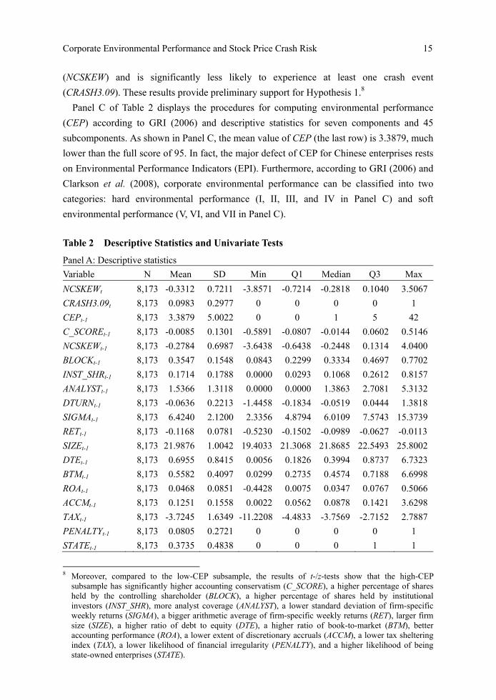
Table 2 presents results of descriptive statistics and univariate tests. As shown in Panel

A of Table 2, the mean value of NCSKEW is -0.3312, which is much larger than the values

reported in Chen et al. (2001) and Kim et al. (2011). This result suggests that my sample of

firm-years is more crash-prone than those in Chen et al. (2001) and Kim et al. (2011). The

mean value of CRASH3.09 is 0.0983, revealing that 9.83% of firm-year observations

experience at least one crash event, lower than reported in Kim et al. (2011). Nevertheless,

the aforementioned mean values are qualitatively similar to those in China-based studies on

crash risk (e.g. Xu et al., 2013, 2014; Chen et al., 2017). CEP has a mean value of 3.3879,

which is quite low compared with the full score of 95, suggesting that Chinese listed firms’

environmental performance is poor. Moreover, the mean value of C_SCORE is -0.0085.

Panel A of Table 2 shows that the distributions of control variables are qualitatively

similar to those in previous studies. On average, the negative conditional return skewness

(NCSKEWt-1) of lagged control variables in this study is -0.2784, the percentage of shares

held by the controlling shareholder (BLOCK) is 35.47%, the percentage of shares held by

institutional investors (INST_SHR) is 17.14%, analyst coverage (ANALYST) is 3.65

(e1.5366-1), the detrended average monthly share turnover (DTURN) is -0.0636, the standard

deviation of firm-specific weekly returns (SIGMA) is 6.4240, the arithmetic average of

firm-specific weekly returns (RET) is -0.1168, firm size (SIZE) is RMB3.5407 billion, the

ratio of debt to equity (DTE) is 69.55%, the book-to-market (BTM) ratio is 0.5582, the

returns on total assets (ROA) are 4.68%, discretionary accruals (ACCM) are 0.1251, the tax

sheltering index (TAX) is -3.7245, the percentage of financial irregularity (PENALTY) is

8.05%, and 37.35% of firms are state-owned enterprises (STATE).

Panel B of Table 2 reports the results of t-/z-tests for differences in the mean (median)

values between the high-CEP subsample (N=2,795) and the low-CEP subsample (N=5,378).

The high-CEP subsample has significantly lower negative conditional return skewness

Corporate Environmental Performance and Stock Price Crash Risk 15

(NCSKEW) and is significantly less likely to experience at least one crash event

(CRASH3.09). These results provide preliminary support for Hypothesis 1.8

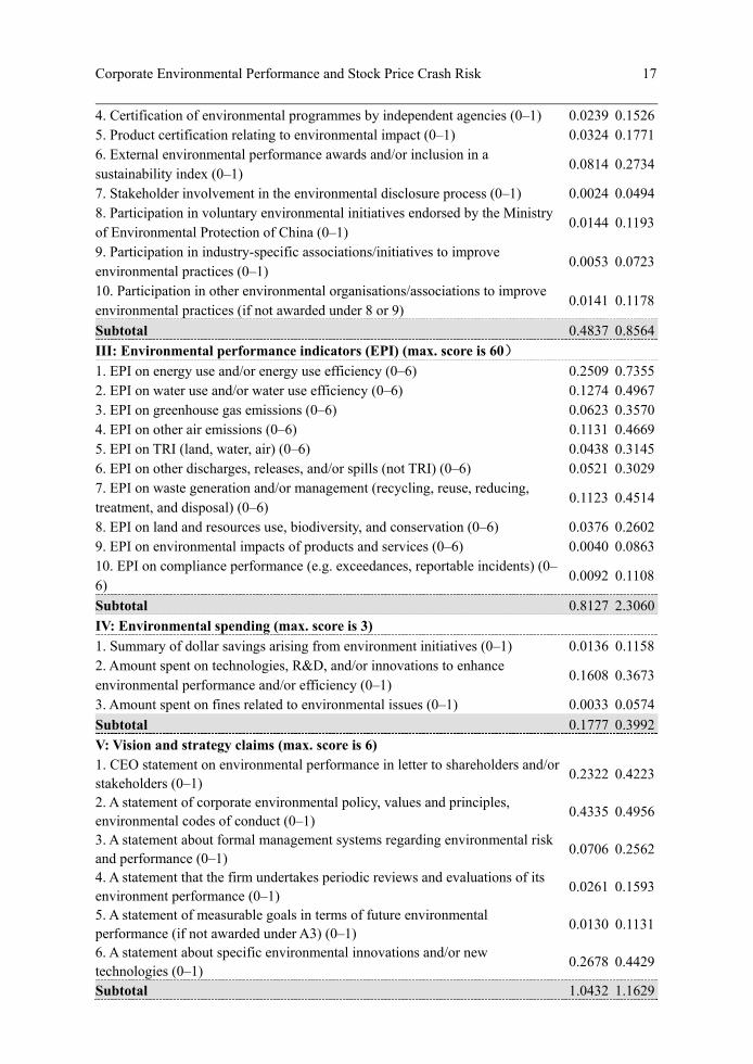
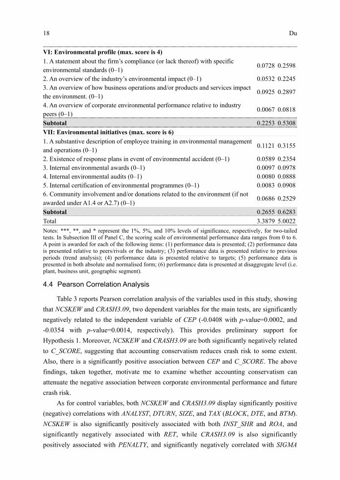
Panel C of Table 2 displays the procedures for computing environmental performance

(CEP) according to GRI (2006) and descriptive statistics for seven components and 45

subcomponents. As shown in Panel C, the mean value of CEP (the last row) is 3.3879, much

lower than the full score of 95. In fact, the major defect of CEP for Chinese enterprises rests

on Environmental Performance Indicators (EPI). Furthermore, according to GRI (2006) and

Clarkson et al. (2008), corporate environmental performance can be classified into two

categories: hard environmental performance (I, II, III, and IV in Panel C) and soft

environmental performance (V, VI, and VII in Panel C).

Table 2 Descriptive Statistics and Univariate Tests

Panel A: Descriptive statistics

Variable N Mean SD Min Q1 Median Q3 Max

NCSKEWt 8,173 -0.3312 0.7211 -3.8571 -0.7214 -0.2818 0.1040 3.5067

CRASH3.09t 8,173 0.0983 0.2977 0 0 0 0 1

CEPt-1 8,173 3.3879 5.0022 0 0 1 5 42

C_SCOREt-1 8,173 -0.0085 0.1301 -0.5891 -0.0807 -0.0144 0.0602 0.5146

NCSKEWt-1 8,173 -0.2784 0.6987 -3.6438 -0.6438 -0.2448 0.1314 4.0400

BLOCKt-1 8,173 0.3547 0.1548 0.0843 0.2299 0.3334 0.4697 0.7702

INST_SHRt-1 8,173 0.1714 0.1788 0.0000 0.0293 0.1068 0.2612 0.8157

ANALYSTt-1 8,173 1.5366 1.3118 0.0000 0.0000 1.3863 2.7081 5.3132

DTURNt-1 8,173 -0.0636 0.2213 -1.4458 -0.1834 -0.0519 0.0444 1.3818

SIGMAt-1 8,173 6.4240 2.1200 2.3356 4.8794 6.0109 7.5743 15.3739

RETt-1 8,173 -0.1168 0.0781 -0.5230 -0.1502 -0.0989 -0.0627 -0.0113

SIZEt-1 8,173 21.9876 1.0042 19.4033 21.3068 21.8685 22.5493 25.8002

DTEt-1 8,173 0.6955 0.8415 0.0056 0.1826 0.3994 0.8737 6.7323

BTMt-1 8,173 0.5582 0.4097 0.0299 0.2735 0.4574 0.7188 6.6998

ROAt-1 8,173 0.0468 0.0851 -0.4428 0.0075 0.0347 0.0767 0.5066

ACCMt-1 8,173 0.1251 0.1558 0.0022 0.0562 0.0878 0.1421 3.6298

TAXt-1 8,173 -3.7245 1.6349 -11.2208 -4.4833 -3.7569 -2.7152 2.7887

PENALTYt-1 8,173 0.0805 0.2721 0 0 0 0 1

STATEt-1 8,173 0.3735 0.4838 0 0 0 1 1

8 Moreover, compared to the low-CEP subsample, the results of t-/z-tests show that the high-CEP

subsample has significantly higher accounting conservatism (C_SCORE), a higher percentage of shares held by the controlling shareholder (BLOCK), a higher percentage of shares held by institutional investors (INST_SHR), more analyst coverage (ANALYST), a lower standard deviation of firm-specific weekly returns (SIGMA), a bigger arithmetic average of firm-specific weekly returns (RET), larger firm size (SIZE), a higher ratio of debt to equity (DTE), a higher ratio of book-to-market (BTM), better accounting performance (ROA), a lower extent of discretionary accruals (ACCM), a lower tax sheltering index (TAX), a lower likelihood of financial irregularity (PENALTY), and a higher likelihood of being state-owned enterprises (STATE).

16 Du

Panel B: t- (z-) tests for differences in the mean (median) value between high- and low-CEP subsamples

The high-CEP subsample

(N=2,795)

The low-CEP subsample

(N=5,378)

Variable Mean Median SD Mean Median SD t-test z-test

NCSKEWt -0.3729 -0.3142 0.7172 -0.3095 -0.2648 0.7222 -3.78*** -3.88***

CRASH3.09t 0.0848 0 0.2786 0.1052 0 0.3069 -3.04*** -2.95***

C_SCOREt-1 0.0580 0.0451 0.1286 -0.0431 -0.0383 0.1167 34.81*** 33.31***

NCSKEWt-1 -0.3091 -0.2660 0.6875 -0.2624 -0.2317 0.7039 -2.87*** -2.94***

BLOCKt-1 0.3881 0.3928 0.1581 0.3374 0.3059 0.1503 13.97*** 14.28***

INST_SHRt-1 0.1931 0.1290 0.1861 0.1602 0.0938 0.1738 7.75*** 10.02***

ANALYSTt-1 2.1530 2.3979 1.2672 1.2163 1.0986 1.2168 32.13*** 30.49***

DTURNt-1 -0.0551 -0.0414 0.1983 -0.0681 -0.0587 0.2322 2.64*** 3.29***

SIGMAt-1 6.1252 5.7074 2.1251 6.5794 6.1436 2.1008 -9.23*** -10.15***

RETt-1 -0.1022 -0.0855 0.0706 -0.1244 -0.1056 0.0807 12.82*** 13.59***

SIZEt-1 22.5136 22.4195 1.1054 21.7142 21.6733 0.8241 33.68*** 31.92***

DTEt-1 0.8404 0.4962 0.9917 0.6202 0.3593 0.7406 10.34*** 10.79***

BTMt-1 0.6499 0.5353 0.4538 0.5105 0.4150 0.3761 13.93*** 15.31***

ROAt-1 0.0601 0.0431 0.0830 0.0400 0.0305 0.0853 10.28*** 10.96***

ACCMt-1 0.1124 0.0823 0.1206 0.1318 0.0913 0.1709 -5.94*** -6.36***

TAXt-1 -3.8026 -3.7350 1.7934 -3.6839 -3.7670 1.5448 -2.97*** 0.72

PENALTYt-1 0.0658 0 0.2480 0.0881 0 0.2835 -3.67*** -3.52***

STATEt-1 0.4182 0 0.4934 0.3503 0 0.4771 5.97*** 6.02***

Panel C: Procedures for computing corporate environmental performance (CEP) Descriptive statistics

Item Mean SD

I: Governance structure and management systems (max. score is 6)

1. Existence of a department for pollution control and/or management positions for environmental management (0–1)

0.1083 0.3108

2. Existence of an environmental and/or a public issues committee in the board (0–1)

0.0064 0.0795

3. Existence of terms and conditions applicable to suppliers and/or customers regarding environmental practices

0.0237 0.1522

4. Stakeholder involvement in setting corporate environmental policies 0.0040 0.0634 5. Implementation of ISO14001 at plant and/or firm level 0.2153 0.4111 6. Executive compensation is linked to environmental performance 0.0221 0.1472

Subtotal 0.3799 0.7024

II: Credibility (max. score is 10)

1. Adoption of GRI sustainability reporting guidelines or provision of a CERES report (0–1)

0.2680 0.4432

2. Independent verification/assurance about environmental information disclosed in the EP report/web

0.0098 0.0985

3. Periodic independent verifications/audits on environmental performance and/or systems (0–1)

0.0321 0.1762

Corporate Environmental Performance and Stock Price Crash Risk 17

4. Certification of environmental programmes by independent agencies (0–1) 0.0239 0.1526 5. Product certification relating to environmental impact (0–1) 0.0324 0.1771 6. External environmental performance awards and/or inclusion in a sustainability index (0–1)

0.0814 0.2734

7. Stakeholder involvement in the environmental disclosure process (0–1) 0.0024 0.0494 8. Participation in voluntary environmental initiatives endorsed by the Ministry of Environmental Protection of China (0–1)

0.0144 0.1193

9. Participation in industry-specific associations/initiatives to improve environmental practices (0–1)

0.0053 0.0723

10. Participation in other environmental organisations/associations to improve environmental practices (if not awarded under 8 or 9)

0.0141 0.1178

Subtotal 0.4837 0.8564

III: Environmental performance indicators (EPI) (max. score is 60）

1. EPI on energy use and/or energy use efficiency (0–6) 0.2509 0.7355 2. EPI on water use and/or water use efficiency (0–6) 0.1274 0.4967 3. EPI on greenhouse gas emissions (0–6) 0.0623 0.3570 4. EPI on other air emissions (0–6) 0.1131 0.4669 5. EPI on TRI (land, water, air) (0–6) 0.0438 0.3145 6. EPI on other discharges, releases, and/or spills (not TRI) (0–6) 0.0521 0.3029 7. EPI on waste generation and/or management (recycling, reuse, reducing, treatment, and disposal) (0–6)

0.1123 0.4514

8. EPI on land and resources use, biodiversity, and conservation (0–6) 0.0376 0.2602 9. EPI on environmental impacts of products and services (0–6) 0.0040 0.0863 10. EPI on compliance performance (e.g. exceedances, reportable incidents) (0–6)

0.0092 0.1108

Subtotal 0.8127 2.3060

IV: Environmental spending (max. score is 3)

1. Summary of dollar savings arising from environment initiatives (0–1) 0.0136 0.1158 2. Amount spent on technologies, R&D, and/or innovations to enhance environmental performance and/or efficiency (0–1)

0.1608 0.3673

3. Amount spent on fines related to environmental issues (0–1) 0.0033 0.0574

Subtotal 0.1777 0.3992

V: Vision and strategy claims (max. score is 6) 1. CEO statement on environmental performance in letter to shareholders and/or stakeholders (0–1)

0.2322 0.4223

2. A statement of corporate environmental policy, values and principles, environmental codes of conduct (0–1)

0.4335 0.4956

3. A statement about formal management systems regarding environmental risk and performance (0–1)

0.0706 0.2562

4. A statement that the firm undertakes periodic reviews and evaluations of its environment performance (0–1)

0.0261 0.1593

5. A statement of measurable goals in terms of future environmental performance (if not awarded under A3) (0–1)

0.0130 0.1131

6. A statement about specific environmental innovations and/or new technologies (0–1)

0.2678 0.4429

Subtotal 1.0432 1.1629

18 Du

VI: Environmental profile (max. score is 4)

1. A statement about the firm’s compliance (or lack thereof) with specific environmental standards (0–1)

0.0728 0.2598

2. An overview of the industry’s environmental impact (0–1) 0.0532 0.2245 3. An overview of how business operations and/or products and services impact the environment. (0–1)

0.0925 0.2897

4. An overview of corporate environmental performance relative to industry peers (0–1)

0.0067 0.0818

Subtotal 0.2253 0.5308

VII: Environmental initiatives (max. score is 6)

1. A substantive description of employee training in environmental management and operations (0–1)

0.1121 0.3155

2. Existence of response plans in event of environmental accident (0–1) 0.0589 0.2354 3. Internal environmental awards (0–1) 0.0097 0.0978 4. Internal environmental audits (0–1) 0.0080 0.0888 5. Internal certification of environmental programmes (0–1) 0.0083 0.0908 6. Community involvement and/or donations related to the environment (if not awarded under A1.4 or A2.7) (0–1)

0.0686 0.2529

Subtotal 0.2655 0.6283

Total 3.3879 5.0022

Notes: ***, **, and * represent the 1%, 5%, and 10% levels of significance, respectively, for two-tailed tests. In Subsection III of Panel C, the scoring scale of environmental performance data ranges from 0 to 6. A point is awarded for each of the following items: (1) performance data is presented; (2) performance data is presented relative to peers/rivals or the industry; (3) performance data is presented relative to previous periods (trend analysis); (4) performance data is presented relative to targets; (5) performance data is presented in both absolute and normalised form; (6) performance data is presented at disaggregate level (i.e. plant, business unit, geographic segment).

4.4 Pearson Correlation Analysis

Table 3 reports Pearson correlation analysis of the variables used in this study, showing

that NCSKEW and CRASH3.09, two dependent variables for the main tests, are significantly

negatively related to the independent variable of CEP (-0.0408 with p-value=0.0002, and

-0.0354 with p-value=0.0014, respectively). This provides preliminary support for

Hypothesis 1. Moreover, NCSKEW and CRASH3.09 are both significantly negatively related

to C_SCORE, suggesting that accounting conservatism reduces crash risk to some extent.

Also, there is a significantly positive association between CEP and C_SCORE. The above

findings, taken together, motivate me to examine whether accounting conservatism can

attenuate the negative association between corporate environmental performance and future

crash risk.

As for control variables, both NCSKEW and CRASH3.09 display significantly positive

(negative) correlations with ANALYST, DTURN, SIZE, and TAX (BLOCK, DTE, and BTM).

NCSKEW is also significantly positively associated with both INST_SHR and ROA, and

significantly negatively associated with RET, while CRASH3.09 is also significantly

positively associated with PENALTY, and significantly negatively correlated with SIGMA

Corporate Environmental Performance and Stock Price Crash Risk 19

T

able

3

Pea

rson

Cor

rela

tion

Mat

rix

Var

iabl

e

(1)

(2)

(3)

(4)

(5)

(6)

(7)

(8)

(9)

(10)

(1

1)

(12)

(1

3)

(14)

(1

5)

(16)

(1

7)

(18)

(1

9)

NC

SKE

Wt

(1)

1

C

RA

SH3.

09t

(2)

0.46

05

(<.0

001)

1

CE

Pt-

1 (3

) -0

.040

8 (0

.000

2)

-0.0

354

(0.0

014)

1

C_S

CO

RE

t-1

(4)

-0.0

654

(<.0

001)

-0

.032

4 (0

.003

4)

0.40

36

(<.0

001)

1

NC

SKE

Wt-

1 (5

) 0.

0598

(<

.000

1)

-0.0

256

(0.0

207)

-0

.023

5 (0

.033

6)

-0.0

420

(0.0

001)

1

BL

OC

Kt-

1 (6

) -0

.052

3 (<

.000

1)

-0.0

325

(0.0

033)

0.

1874

(<

.000

1)

0.28

89

(<.0

001)

-0

.056

0 (<

.000

1)

1

INST

_SH

Rt-

1 (7

) 0.

0603

(<

.000

1)

-0.0

081

(0.4

626)

0.

0681

(<

.000

1)

0.13

42

(<.0

001)

0.

0809

(<

.000

1)

0.00

07

(0.9

488)

1

AN

AL

YST

t-1

(8)

0.08

83

(<.0

001)

0.

0182

(0

.099

2)

0.35

49

(<.0

001)

0.

5542

(<

.000

1)

0.09

53

(<.0

001)

0.

1887

(<

.000

1)

0.23

66

(<.0

001)

1

DT

UR

Nt-

1 (9

) 0.

0854

(<

.000

1)

0.06

93

(<.0

001)

0.

0251

(0

.023

4)

0.00

75

(0.4

989)

-0

.191

0 (<

.000

1)

-0.0

219

(0.0

477)

-0

.015

7 (0

.156

3)

0.05

32

(<.0

001)

1

SIG

MA

t-1

(10)

0.

0094

(0

.394

6)

-0.0

593

(<.0

001)

-0

.162

1 (<

.000

1)

-0.0

901

(<.0

001)

-0

.059

3 (<

.000

1)

-0.0

312

(0.0

048)

-0

.011

6 (0

.296

0)

-0.1

375

(<.0

001)

0.

0493

(<

.000

1)

1

RE

Tt-

1 (1

1)

-0.0

694

(<.0

001)

0.

0159

(0

.149

7)

0.16

69

(<.0

001)

0.

1855

(<

.000

1)

0.08

88

(<.0

001)

0.

0474

(<

.000

1)

-0.0

076

(0.4

903)

0.

1219

(<

.000

1)

-0.2

064

(<.0

001)

-0

.829

2 (<

.000

1)

1

SIZ

Et-

1 (1

2)

0.05

40

(<.0

001)

0.

0309

(0

.005

3)

0.43

44

(<.0

001)

0.

6698

(<

.000

1)

-0.0

607

(<.0

001)

0.

2100

(<

.000

1)

0.17

94

(<.0

001)

0.

6415

(<

.000

1)

0.14

86

(<.0

001)

-0

.273

4 (<

.000

1)

0.17

15

(<.0

001)

1

DT

Et-

1 (1

3)

-0.1

540

(<.0

001)

-0

.047

5 (<

.000

1)

0.15

41

(<.0

001)

0.

3443

(<

.000

1)

-0.0

608

(<.0

001)

0.

1361

(<

.000

1)

-0.0

322

(0.0

036)

0.

0558

(<

.000

1)

-0.0

656

(<.0

001)

-0

.142

2 (<

.000

1)

0.20

32

(<.0

001)

0.

0513

(<

.000

1)

1

BT

Mt-

1 (1

4)

-0.2

027

(<.0

001)

-0

.088

0 (<

.000

1)

0.17

79

(<.0

001)

0.

4290

(<

.000

1)

-0.0

340

(0.0

021)

0.

2381

(<

.000

1)

-0.0

117

(0.2

919)

0.

0734

(<

.000

1)

-0.1

502

(<.0

001)

-0

.044

9 (<

.000

1)

0.22

43

(<.0

001)

-0

.069

9 (<

.000

1)

0.53

50

(<.0

001)

1

RO

At-

1 (1

5)

0.06

69

(<.0

001)

0.

0064

(0

.561

5)

0.09

32

(<.0

001)

0.

2798

(<

.000

1)

0.04

28

(0.0

001)

0.

1547

(<

.000

1)

0.16

72

(<.0

001)

0.

4299

(<

.000

1)

0.03

11

(0.0

050)

-0

.074

7 (<

.000

1)

0.03

24

(0.0

034)

0.

3557

(<

.000

1)

-0.2

015

(<.0

001)

-0

.051

2 (<

.000

1)

1

AC

CM

t-1

(16)

0.

0125

(0

.259

0)

0.00

59

(0.5

908)

-0

.053

3 (<

.000

1)

-0.0

030

(0.7

876)

0.

0199

(0

.072

4)

0.03

24

(0.0

034)

0.

0030

(0

.785

5)

-0.0

263

(0.0

175)

-0

.002

4 (0

.830

1)

-0.0

152

(0.1

708)

-0

.010

6 (0

.336

2)

-0.0

147

(0.1

838)

0.

0363

(0

.001

0)

0.01

72

(0.1

209)

0.

1098

(<

.000

1)

1

TA

Xt-

1 (1

7)

0.14

04

(<.0

001)

0.

0444

(0

.000

1)

-0.0

555

(<.0

001)

-0

.085

4 (<

.000

1)

0.06

50

(<.0

001)

-0

.039

0 (0

.000

4)

0.05

35

(<.0

001)

0.

0877

(<

.000

1)

0.01

42

(0.2

001)

0.

1667

(<

.000

1)

-0.1

769

(<.0

001)

0.

0865

(<

.000

1)

-0.7

201

(<.0

001)

-0

.384

7 (<

.000

1)

0.40

33

(<.0

001)

0.

0737

(<

.000

1)

1

PE

NA

LT

Yt-

1

(18)

0.

0165

(0

.136

8)

0.02

17

(0.0

501)

-0

.033

6 (0

.002

4)

-0.1

092

(<.0

001)

0.

0117

(0

.288

7)

-0.0

435

(0.0

001)

-0

.018

0 (0

.103

2)

-0.0

885

(<.0

001)

0.

0198

(0

.073

6)

-0.0

456

(<.0

001)

-0

.012

7 (0

.250

5)

-0.0

657

(<.0

001)

0.

0103

(0

.349

7)

-0.0

507

(<.0

001)

-0

.057

3 (<

.000

1)

0.04

09

(0.0

002)

-0

.043

9 (0

.000

1)

1

STA

TE

t-1

(19)

0.

0074

(0

.506

1)

-0.0

229

(0.0

388)

0.

0360

(0

.001

1)

0.20

23

(<.0

001)

0.

0421

(0

.000

1)

0.15

98

(<.0

001)

0.

0264

(0

.017

0)

0.06

94

(<.0

001)

-0

.086

7 (<

.000

1)

0.26

54

(<.0

001)

-0

.105

8 (<

.000

1)

0.04

90

(<.0

001)

-0

.001

9 (0

.866

1)

0.04

35

(0.0

001)

-0

.006

5 (0

.557

9)

-0.0

643

(<.0

001)

0.

1458

(<

.000

1)

-0.1

132

(<.0

001)

1

Not

e: p

-val

ues

are

pres

ente

d in

par

enth

eses

bel

ow t

he c

oeff

icie

nt v

alue

s. A

ll v

aria

bles

are

def

ined

in

App

endi

x I.

20 Du

and STATE, respectively. These results, taken together, suggest a need to control for these

variables when I examine the influence of corporate environmental performance (CEP) on

stock price crash risk. Moreover, as expected, the coefficients of pair-wise correlation

among other control variables are generally low, suggesting that there is no serious

multicollinearity when these variables are included in the regression simultaneously.

V. Empirical Results

Table 4 reports the results of OLS regression in Section A and the logistic regression in

Section B, in which NCSKEW and CRASH3.09 are dependent variables, respectively. To

mitigate the potential problem of autocorrelation and clustering in the sample, all reported

t-values are based on standard errors adjusted for clustering at the firm level (Petersen,

2009). Table 4 reports the step-by-step regression results of stock price crash risk on

corporate environmental performance, accounting conservatism, and other determinants. All

models are highly significant (F-/LR-statistics). Four step-by-step regressions display

gradually increasing explanatory power with significantly higher adj_R2 or Pseudo_R2 (see

R2 between nearby models and results of F-/Chi-squared tests in the second to last row).

5.1 Results Using NCSKEW as the Dependent Variable

Column (1) of Section A in Table 4 reports the regression results of stock price crash

risk on all control variables. Those in Column (1) reveal the following:

1. The coefficient on BLOCK is negative and significant, implying a negative association

between the percentage of shares held by the controlling shareholder and negatively skewed

future return distribution.

2. The coefficient on INST_SHR is positive and significant, suggesting that a higher

proportion of shares held by institutional investors brings out more negatively skewed future

return distribution. This result is consistent with the findings of Kim et al. (2011).

3. ANALYST has a positive and significant coefficient, which is also consistent with Kim et

al. (2011).

4. The coefficient on SIGMA is significantly negative.

5. RET has a significantly negative coefficient, revealing that the arithmetical average of

firm-specific weekly returns is negatively associated with the extent of a firm’s future

negative return skewness.

6. TAX has a positive and significant coefficient, which suggests that the extent of

negatively skewed future returns is positively associated with tax avoidance, echoing the

findings in Kim et al. (2011).

The sign and significance of SIGMA, RET, SIZE, and DTE are different from those

reported in Kim et al. (2014) and Kim and Zhang (2016). Nevertheless, they are

qualitatively similar to those reported in several China-based studies on crash risk (Chen et

Corporate Environmental Performance and Stock Price Crash Risk 21

al., 2017; Xu et al., 2013, 2014). These disparities can be explained by the differences in the

institutional setting between China and Western economies (markets). For example, in

China’s stock market, changes in daily prices are not allowed to exceed +/-10% of the

previous closing price.

Column (2) of Section A in Table 4 reports the regression results of NCSKEW on

corporate environmental performance and other determinants. The coefficient on CEP is

negative and significant at the 1% level (-0.0052 with t=-3.15), providing strong support for

Hypothesis 1. This suggests that environmentally friendly firms engage in less bad news

hoarding and present a higher degree of information transparency than environmentally

irresponsible firms, and thus their firm-specific return distributions are less negatively

skewed in the future. Also, the coefficient estimate suggests that an increase of one standard

deviation in CEP reduces firm-specific future negative return skewness by about 2.60%,

equal to about 7.85% of the mean value of NCSKEW. Clearly, this amount is economically

significant, in addition to its statistical significance.

Column (3) of Section A in Table 4 reports the effects of stock price crash risk on

corporate environmental performance, accounting conservatism, and all control variables.

Consistent with Hypothesis 1, CEP has a negative and significant coefficient at the 1% level

(-0.0044 and t=-2.64). The coefficient on C_SCORE is also negative and significant at the 1%

level (-0.5572 with t=-5.40), suggesting that firms with higher scores for accounting

conservatism experience less future negative return skewness. This finding is supported by

Kim and Zhang (2016).

Column (4) of Section A in Table 4 reports the regression results of Hypothesis 2. It

shows that the coefficient on CEP×C_SCORE is positive and significant at the 1% level

(0.0308 with t=3.14), lending significant support to Hypothesis 2. This result validates that

accounting conservatism attenuates the negative association between corporate

environmental performance and stock price crash risk. Moreover, both CEP and C_SCORE

have significantly negative coefficients, echoing Hypothesis 1 again and consistent with

Kim and Zhang (2016), respectively.

5.2 Results Using CRASH3.09 as the Dependent Variable

Column (5) of Section B in Table 4 reports the effect of all control variables on stock

price crash risk. Briefly, the likelihood of future crash risk (CRASH3.09) is significantly

negatively related to SIGMA, RET, and STATE, but significantly positively related to

ANALYST, DTE, and PENALTY. These results are qualitatively similar to those in Chen et al.

(2001) and Kim et al. (2011).

Column (6) of Section B in Table 4 reports the results relating to Hypothesis 1. The

coefficient on CEP is negative and significant at the 1% level (-0.0288 with t=-2.73),

providing strong support for Hypothesis 1 again and suggesting that firms with better

environmental performance are significantly less likely to experience future crash risk than

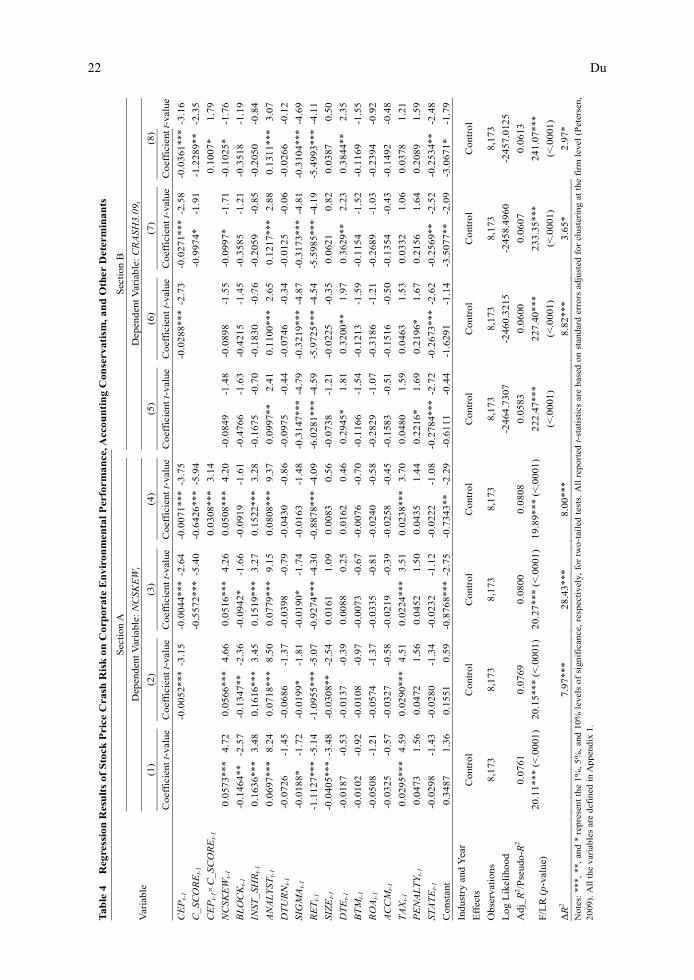
22 Du

Tab

le 4

R

egre

ssio

n R

esu

lts

of S

tock

Pri

ce C

rash

Ris

k o

n C

orp

orat

e E

nvi

ron

men

tal

Per

form

ance

, Acc

oun

tin

g C

onse

rvat

ism

, an

d O

ther

Det

erm

inan

ts

Var

iab

le

S

ecti

on A

Sec

tion

B

D

epen

den

t V

aria

ble:

NC

SKE

Wt

D

epen

dent

Var

iab

le:

CR

ASH

3.0

9 t

(1

)

(2)

(3

)

(4)

(5

)

(6)

(7

)

(8)

C

oeff

icie

nt t

-val

ue

Coe

ffic

ient

t-v

alue

C

oeff

icie

nt t

-val

ue

Coe

ffic

ient

t-v

alue

C

oef

fici

ent

t-va

lue

Co

effi

cien

t t-

valu

e C

oef

fici

ent

t-va

lue

Co

effi

cien

t t-v

alue

CE

Pt-

1

-

0.0

052*

**-3

.15

-

0.0

044*

**-2

.64

-0.

0071

***

-3.7

5

-0

.02

88**

* -2

.73

-0

.027

1***

-2.5

8 -

0.0

361*

**-3

.16

C_S

CO

RE

t-1

-0.

557

2***

-5.4

0 -

0.64

26**

*-5

.94

-0

.997

4*

-1.9

1

-1.2

289*

* -2

.35

CE

Pt-

1×C

_SC

OR

Et-

1

0.0

308

***

3.1

4

0.

100

7*

1.79

NC

SK

EW

t-1

0

.05

73**

*4.

72

0

.05

66**

*4.

66

0.

0516

***

4.2

6

0.0

508

***

4.2

0

-0.0

849

-1.4

8

-0.0

898

-1.5

5

-0.0

997*

-1

.71

-0

.102

5*

-1.7

6

BL

OC

Kt-

1

-0

.14

64**

-2

.57

-0.1

347

**

-2.3

6

-0

.09

42*

-1.6

6

-0.0

919

-1

.61

-0

.476

6 -1

.63

-0

.421

5 -1

.45

-0

.358

5 -1

.21

-0

.351

8 -1

.19

INST

_SH

Rt-

1

0.1

636

***

3.48

0.1

616

***

3.45

0.15

19**

*3.

27

0

.15

22**

*3

.28

-0

.167

5 -0

.70

-0

.183

0 -0

.76

-0

.205

9 -0

.85

-0

.205

0 -0

.84

AN

AL

YS

Tt-

1

0

.06

97**

*8.

24

0

.07

18**

*8.

50

0.

0779

***

9.1

5

0.0

808

***

9.3

7

0.0

997

**

2.4

1

0.1

100

***

2.6

5

0.12

17**

*2.

88

0.

131

1***

3.07

DT

UR

Nt-

1

-0

.07

26

-1.4

5

-0

.06

86

-1.3

7

-0

.03

98

-0.7

9

-0.0

430

-0

.86

-0

.097

5 -0

.44

-0

.074

6 -0

.34

-0

.012

5 -0

.06

-0

.026

6 -0

.12

SIG

MA

t-1

-0

.018

8*

-1.7

2

-0.0

199*

-1

.81

-0

.019

0*

-1.7

4

-0.0

163

-1.4

8 -

0.3

147*

**-4

.79

-0

.321

9***

-4

.87

-0

.317

3***

-4.8

1 -

0.3

104*

**-4

.69

RE

Tt-

1

-1.1

127*

**-5

.14

-

1.0

955*

**-5

.07

-

0.9

274*

**-4

.30

-0.

8878

***

-4.0

9 -

6.0

281

***

-4.5

9 -

5.9

725

***

-4.5

4 -

5.5

985*

**-4

.19

-5

.499

3***

-4.1

1

SIZ

Et-

1

-0.0

405*

**-3

.48

-0.0

308

**

-2.5

4

0.

0161

1.

09

0

.00

83

0.5

6

-0.0

738

-1.2

1

-0.0

225

-0.3

5

0.0

621

0.8

2

0.0

387

0.50

DT

Et-

1

-0

.018

7 -0

.53

-0

.013

7 -0

.39

0.

0088

0.

25

0.

0162

0.

46

0.

2945

* 1.

81

0.

3200

**

1.97

0.36

29**

2.

23

0.

3844

**

2.35

BT

Mt-

1

-0

.01

02

-0.9

2

-0

.01

08

-0.9

7

-0

.00

73

-0.6

7

-0.0

076

-0

.70

-0

.116

6 -1

.54

-0

.121

3 -1

.59

-0

.115

4 -1

.52

-0

.116

9 -1

.55

RO

At-

1

-0.0

508

-1

.21

-0.0

574

-1

.37

-0.0

335

-0

.81

-0

.02

40

-0.5

8

-0.2

829

-1.0

7

-0.3

186

-1.2

1

-0.2

689

-1.0

3

-0.2

394

-0.9

2

AC

CM

t-1

-0

.03

25

-0.5

7

-0

.03

27

-0.5

8

-0

.02

19

-0.3

9

-0.0

258

-0

.45

-0

.158

3 -0

.51

-0

.151

6 -0

.50

-0

.135

4 -0

.43

-0

.149

2 -0

.48

TA

Xt-

1

0.0

295

***

4.59

0.0

290

***

4.51

0.02

24**

*3.

51

0

.02

38**

*3

.70

0.

048

0 1

.59

0

.046

3 1

.53

0.

033

2 1.

06

0.

037

8 1.

21

PE

NA

LT

Yt-

1

0.

0473

1.

56

0.

0472

1.

56

0.

0452

1.

50

0

.04

35

1.4

4

0.2

216

* 1

.69

0

.219

6*

1.6

7

0.2

156

1.6

4

0.2

089

1.59

ST

AT

Et-

1

-0.0

298

-1

.43

-0.0

280

-1

.34

-0.0

232

-1

.12

-0

.02

22

-1.0

8 -

0.2

784

***

-2.7

2 -

0.2

673

***

-2.6

2

-0.2

569*

* -2

.52

-0

.253

4**

-2.4

8

Con

stan

t

0.34

87

1.36

0.15

51

0.59

-

0.8

768*

**-2

.75

-0

.73

43**

-2

.29

-0

.611

1 -0

.44

-1

.629

1 -1

.14

-3

.507

7**

-2.0

9

-3.0

671*

-1

.79

Indu

stry

and

Yea

r

Eff

ects

C

ontr

ol

C

ontr

ol

C

ontr

ol

C

ontr

ol

C

ont

rol

C

ont

rol

C

ont

rol

C

ontr

ol

Obs

erva

tion

s

8,1

73

8,

173

8,

173

8,

173

8,1

73

8

,173

8,1

73

8,

173

Log

Lik

elih

ood

-246

4.7

307

-2

460

.321

5

-245

8.49

60

-2

457.

012

5

Ad

j_R

2 /Pse

udo

-R2

0

.07

61

0

.07

69

0

.08

00

0

.080

8

0.0

583

0.

060

0

0.06

07

0

.06

13

F/L

R (

p-v

alue

)

20.1

1***

(<

.00

01)

20

.15

***

(<.0

001

) 2

0.2

7**

* (<

.00

01)

19.

89*

** (

<.0

001

)

222

.47

***

(<.0

001

)

2

27.4

0**

*

(<.0

001

)

23

3.35

***

(<.0

001)

24

1.07

***

(<.0

001

)

ΔR

2

7.

97**

*

28.4

3**

*

8.0

0**

*

8

.82*

**

3.

65*

2.97

* N

otes

: **

*, *

*, a

nd *

rep

rese

nt t

he 1

%,

5%,

and

10%

lev

els

of s

igni

fica

nce,

res

pect

ivel

y, f

or t

wo-

tail

ed t

ests

. A

ll r

epor

ted

t-s

tati

stic

s ar

e ba

sed

on s

tand

ard

erro

rs a

djus

ted

for

clus

teri

ng a

t th

e fi

rm l

evel

(P

eter

sen,

2009

). A

ll t

he v

aria

bles

are

def

ined

in

App

endi

x 1.

Corporate Environmental Performance and Stock Price Crash Risk 23

firms with worse environmental performance.

Column (7) of Section B in Table 4 shows the significantly negative influence of

environmental performance on the likelihood of future crash risk after including accounting

conservatism (-0.0271 with t=-2.58). Moreover, the coefficient on C_SCORE is negative

and significant (-0.9974 with t=-1.91), consistent with Hypothesis 1 and the findings of Kim

and Zhang (2016).

Column (8) of Section B in Table 4 reports the results relating to Hypothesis 2. The

coefficient on CEP×C_SCORE is positive and significant at the 10% level (0.1007 with

t=1.79), lending significant support to Hypothesis 2. This result validates the moderating

role of accounting conservatism and the substitutive effects between corporate

environmental performance and accounting conservatism reducing the likelihood of future

stock price crash risk.

VI. Robustness Checks

6.1 Robustness Checks Using Alternative Measures of Stock Price Crash Risk

To ensure that the results in Table 4 are robust to other measures of crash risk, I

construct a set of additional proxies for crash risk to retest Hypotheses 1 and 2.

First, I compute DUVOLj,t and CRASHN3.09j,t as two additional variables to retest the

hypotheses. DUVOLj,t captures asymmetric volatility between negative and positive

firm-specific weekly returns and the down-to-up volatility of the likelihood of future stock

price crash risk for firm j in year t. DUVOLj,t is measured following Eq. (9):

DOWN UPtjdtjutj WnWnDUVOL 2,

2,, )1(/)1(log , (9)

where nu is the number of weeks in which Wj,t is greater than the annual mean value of Wj,t,

and nd is the number of weeks in which Wj,t is lower than the annual mean value of Wj,t (Kim

et al., 2011).

This study also computes the number of stock price crashes for firm j in year t, labelled

CRASHN3.09j,t, as another alternative dependent variable with which to conduct robustness

checks.

Panel A of Table 5 provides results using DUVOLj,t and CRASHN3.09j,t as dependent

variables. In Columns (2) and (6) of Panel A, the coefficients on CEP are both negative and

significant (-0.0036 with t=-3.19 and -0.0288 with t=-2.73), providing strong additional

evidence for Hypothesis 1. In Columns (4) and (8) of Panel A, the coefficients on

CEP×C_SCORE are both significantly positive (0.0169 with t=2.47 and 0.1011 with t=1.80),

lending significant additional evidence for Hypothesis 2. Also, both CEP and C_SCORE in

Columns (4) and (8) of Panel A are negative and significant, consistent with Hypothesis 1

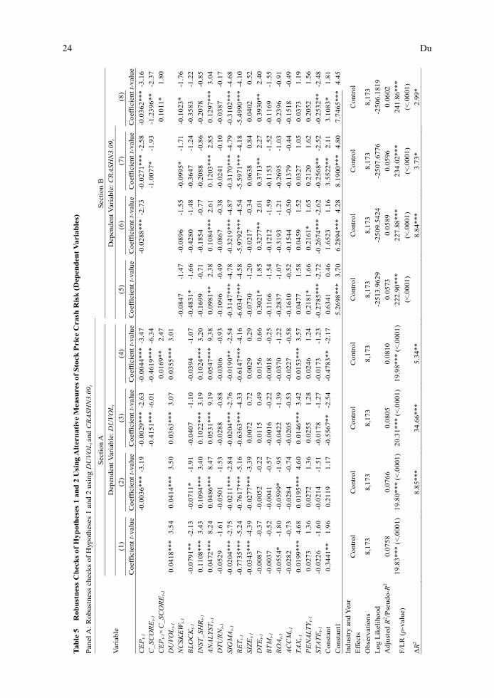
24 Du

Tab

le 5

R

obu

stn

ess

Ch

eck

s of

Hyp

oth

eses

1 a

nd

2 U

sin

g A

lter

nat

ive

Mea

sure

s of

Sto

ck P

rice

Cra

sh R

isk

(D

epen

den

t V

aria

ble

s)

Pan

el A

: R

obus

tnes

s ch

ecks

of

Hyp

othe

ses

1 an

d 2

usin

g D

UV

OL

t an

d C

RA

SHN

3.09

t

Var

iabl

e

S

ecti

on A

Sec

tion

B

D

epen

dent

Var

iabl

e: D

UV

OL

t

Dep

ende

nt V

aria

ble:

CR

ASH

N3.

09t

(1

)

(2)

(3

)

(4)

(5

)

(6)

(7

)

(8)

C

oeff

icie

nt t

-val

ue

Coe

ffic

ient

t-v

alue

C

oeff

icie

nt t

-val

ue

Coe

ffic

ient

t-v

alue

C

oeff

icie

nt t

-val

ue

Coe

ffic

ient

t-v

alue

C

oeff

icie

nt t

-val

ue

Coe

ffic

ient

t-va

lue

CE

Pt-

1

-

0.00

36**

*-3

.19

-0.

0029

***

-2.6

3 -

0.00

44**

*-3

.47

-

0.02

88**

* -2

.73

-0.

0271

***

-2.5

8 -

0.03

62**

*-3

.16

C_S

CO

RE

t-1

-0.

4151

***

-6.0

1 -

0.46

19**

*-6

.34

-1

.007

7*

-1.9

3

-1.2

396*

* -2

.37

CE

Pt-

1×C

_SC

OR

Et-

1

0.01

69**

2.

47

0.10

11*

1.80

DU

VO

Lt-

1

0.

0418

***

3.54

0.04

14**

*3.

50

0.

0363

***

3.07

0.03

55**

*3.

01

NC

SKE

Wt-

1

-0

.084

7 -1

.47

-0

.089

6 -1

.55

-0

.099

5*

-1.7

1

-0.1

023*

-1

.76

BL

OC

Kt-

1

-0

.079

1**

-2.1

3

-0.0

711*

-1

.91

-0

.040

7 -1

.10

-0

.039

4 -1

.07

-0

.483

1*

-1.6

6

-0.4

280

-1.4

8

-0.3

647

-1.2

4

-0.3

583

-1.2

2

INST

_SH

Rt-

1

0.11

08**

*3.

43

0.

1094

***

3.40

0.10

22**

* 3.

19

0.

1024

***

3.20

-0.1

699

-0.7

1

-0.1

854

-0.7

7

-0.2

088

-0.8

6

-0.2

078

-0.8

5

AN

AL

YST

t-1

0.

0472

***

8.24

0.04

86**

*8.

47

0.

0531

***

9.19

0.05

47**

*9.

38

0.

0981

**

2.38

0.10

84**

* 2.

61

0.

1203

***

2.85

0.12

97**

*3.

04

DT

UR

Nt-

1

-0

.052

9 -1

.61

-0

.050

1 -1

.53

-0

.028

8 -0

.88

-0

.030

6 -0

.93

-0

.109

6 -0

.49

-0

.086

7 -0

.38

-0

.024

1 -0

.10

-0

.038

7 -0

.17

SIG

MA

t-1

-0

.020

4***

-2.7

5 -

0.02

11**

*-2

.84

-0.

0204

***

-2.7

6

-0.0

190*

* -2

.54

-0.

3147

***

-4.7

8 -

0.32

19**

* -4

.87

-0.

3170

***

-4.7

9 -

0.3

102*

**-4

.68

RE

Tt-

1

-0.7

735*

**-5

.24

-0.

7617

***

-5.1

6 -

0.63

63**

* -4

.33

-0.

6147

***

-4.1

6 -

6.03

47**

*-4

.58

-5.

9792

***

-4.5

4 -

5.59

71**

* -4

.18

-5.

4990

***

-4.1

0

SIZ

Et-

1

-0.0

343*

**-4

.39

-0.

0277

***

-3.3

9

0.00

72

0.72

0.00

29

0.29

-0.0

730

-1.2

0

-0.0

217

-0.3

4

0.06

38

0.84

0.04

02

0.52

DT

Et-

1

-0

.008

7 -0

.37

-0

.005

2 -0

.22

0.

0115

0.

49

0.

0156

0.

66

0.

3021

* 1.

85

0.

3277

**

2.01

0.37

13**

2.

27

0.

3930

**

2.40

BT

Mt-

1

-0

.003

7 -0

.52

-0

.004

1 -0

.57

-0

.001

6 -0

.22

-0

.001

8 -0

.25

-0

.116

6 -1

.54

-0

.121

2 -1

.59

-0

.115

3 -1

.52

-0

.116

9 -1

.55

RO

At-

1

-0.0

554*

-1

.80

-0

.059

9*

-1.9

5

-0.0

422

-1.3

9

-0.0

370

-1.2

2

-0.2

837

-1.0

7

-0.3

193

-1.2

1

-0.2

695

-1.0

3

-0.2

396

-0.9

1

AC

CM

t-1

-0

.028

2 -0

.73

-0

.028

4 -0

.74

-0

.020

5 -0

.53

-0

.022

7 -0

.58

-0

.161

0 -0

.52

-0

.154

4 -0

.50

-0

.137

9 -0

.44

-0

.151

8 -0

.49

TA

Xt-

1

0.01

99**

*4.

68

0.

0195

***

4.60

0.01

46**

* 3.

42

0.

0153

***

3.57

0.04

77

1.58

0.04

59

1.52

0.03

27

1.05

0.03

73

1.19

PE

NA

LT

Yt-

1

0.

0273

1.

36

0.

0272

1.

36

0.

0255

1.

28

0.

0246

1.

24

0.

2181

* 1.

66

0.

2161

* 1.

65

0.

2120

1.

62

0.

2052

1.

56

STA

TE

t-1

-0

.022

6 -1

.60

-0

.021

4 -1

.51

-0

.017

8 -1

.27

-0

.017

3 -1

.23

-0.

2785

***

-2.7

2 -

0.26

74**

* -2

.62

-0

.256

8**

-2.5

2

-0.2

532*

* -2

.48

Con

stan

t

0.34

41**

1.

96

0.

2119

1.

17

-0

.556

7**

-2.5

4

-0.4

783*

* -2

.17

0.

6341

0.

46

1.

6523

1.

16

3.

5522

**

2.11

3.10

83*

1.81

Con

stan

t1

5.

2698

***

3.70

6.28

94**

* 4.

28

8.

1900

***

4.80

7.74

65**

*4.

45

Indu

stry

and

Yea

r

Eff

ects

C

ontr

ol

C

ontr

ol

C

ontr

ol

C

ontr

ol

C

ontr

ol

C

ontr

ol

C

ontr

ol

C

ontr

ol

Obs

erva

tion

s

8,17

3

8,17

3

8,17

3

8,17

3

8,17

3

8,17

3

8,17

3

8,17

3

Log

Lik

elih

ood

-2

513.

9629

-250

9.54

24

-2

507.

6776

-250

6.18

19

Adj

uste

d R

2 /Pse

udo-

R2

0.07

58

0.

0766

0.08

05

0.

0810

0.05

73

0.

0589

0.05

96

0.

0602

F/L

R (

p-va

lue)

19.8

3***

(<

.000

1)

19.8

0***

(<

.000

1)

20.3

1***

(<

.000

1)

19.9

8***

(<

.000

1)

222.

90**

*

(<.0

001)

22

7.88

***

(<.0

001)

23

4.02

***

(<.0

001)

24

1.86

***

(<.0

001)

ΔR

2

8.

85**

*

34.6

6***

5.34

**

8.

84**

*

3.73

*

2.99

*

Corporate Environmental Performance and Stock Price Crash Risk 25

Pan

el B

: Rob

ustn

ess

chec

ks u

sing

CR

ASH

2.90

t and

CR

ASH

3.00

t

Var

iabl

e

S

ecti

on A

Sec

tion

B

D

epen

dent

Var

iabl

e: C

RA

SH2.

90t

D

epen

dent

Var

iabl

e: C

RA

SH3.

00t

(1

)

(2)

(3

)

(4)

(5

)

(6)

(7

)

(8)

C

oeff

icie

nt t-

valu

e C

oeff

icie

nt t-

valu

e C

oeff

icie

nt t

-val

ue

Coe

ffic

ient

t-va

lue

Coe

ffic

ient

t-v

alue

C

oeff

icie

nt t-

valu

e C

oeff

icie

nt t

-val

ue

Coe

ffic

ient

t-va

lue

CE

Pt-

1

-0.

0218

***

-2.6

1 -

0.01

99**

-2

.38

-0.

0234

***

-2.5

9

-0.

0262

***

-2.7

7 -

0.02

39**

-2

.54

-0.

0291

***

-2.8

9

C_S

CO

RE

t-1

-1.

1499

***

-2.6

4 -

1.25

06**

*-2

.82

-1.

3665

***

-2.8

5 -

1.50

96**

* -3

.11

CE

Pt-

1×C

_SC

OR

Et-

1

0.04

38*

1.68

0.

0650

**

2.08

NC

SKE

Wt-

1

-0.0

445

-0.9

0 -

0.04

78

-0.9

6 -

0.05

93

-1.1

8 -

0.06

03

-1.2

1 -

0.05

81

-1.0

9 -

0.06

23

-1.1

6 -

0.07

63

-1.4

1 -

0.07

79

-1.4

3

BL

OC

Kt-

1

-0

.654

7***

-2.6

6 -

0.61

05**

-2

.48

-0.

5349

**

-2.1

6 -

0.53

09**

-2

.14

-0.

5420

**

-2.0

8 -

0.49

04*

-1.8

8 -

0.40

12

-1.5

3 -

0.39

65

-1.5

1

INST

_SH

Rt-

1

0.03

21

0.16

0.02

13

0.11

-

0.00

29

-0.0

1 -

0.00

20

-0.0

1 -

0.06

12

-0.2

8 -

0.07

52

-0.3

5 -

0.10

62

-0.4

8 -

0.10

50

-0.4

8

AN

AL

YST

t-1

0.

0735

**

2.14

0.08

17**

2.

37

0.

0955

***

2.72

0.09

93**

*2.

80

0.

0847

**

2.28

0.09

45**

2.

53

0.

1111

***

2.93

0.11

68**

* 3.

05

DT

UR

Nt-

1

0.04

69

0.23

0.06

38

0.31

0.13

29

0.63

0.12

74

0.61

-

0.01

91

-0.0

9

0.00

10

0.00

0.08

40

0.39

0.07

54

0.35

SIG

MA

t-1

-0

.292

1***

-5.2

5 -

0.29

73**

*-5

.32

-0.

2924

***

-5.2

5 -

0.28

95**

*-5

.18

-0.

2951

***

-4.9

2 -

0.30

15**

* -5

.01

-0.

2954

***

-4.9

1 -

0.29

10**

* -4

.84

RE

Tt-

1

-5.5

237*

**-5

.00

-5.

4767

***

-4.9

6 -

5.05

21**

*-4

.53

-5.

0111

***

-4.4

8 -

5.76

09**

*-4

.83

-5.

7119

***

-4.7

9 -

5.19

63**

* -4

.30

-5.

1376

***

-4.2

5

SIZ

Et-

1

-0.0

893*

-1

.81

-0.

0508

-0

.99

0.

0468

0.

77

0.

0360

0.

57

-0.

1017

* -1

.87

-0.

0561

-0

.99

0.

0603

0.

89

0.

0444

0.

64

DT

Et-

1

0.10

74

0.77

0.12

67

0.91

0.17

69

1.26

0.18

65

1.32

0.28

69*

1.92

0.30

98**

2.

08

0.

3701

**

2.48

0.38

38**

2.

56

BT

Mt-

1

-0

.064

5 -1

.05

-0.

0676

-1

.09

-0.

0616

-1

.01

-0.

0624

-1

.02

-0.

0701

-1

.05

-0.

0739

-1

.10

-0.

0665

-1

.01

-0.

0677

-1

.03

RO

At-

1

-0.2

791

-1.2

8 -

0.30

48

-1.4

1 -

0.24

71

-1.1

5 -

0.23

43

-1.0

9 -

0.38

85*

-1.6

7 -

0.41

88*

-1.8

1 -

0.34

72

-1.5

0 -

0.32

87

-1.4

2

AC

CM

t-1

-0

.238

8 -0

.90

-0.

2335

-0

.89

-0.

2158

-0

.81

-0.

2225

-0

.83

-0.

1680

-0

.61

-0.

1625

-0

.59

-0.

1394

-0

.50

-0.

1483

-0

.53

TA

Xt-

1

0.03

12

1.24

0.02

94

1.17

0.01

41

0.54

0.01

62

0.62

0.04

24

1.57

0.04

06

1.50

0.02

25

0.80

0.02

55

0.90

PE

NA

LT

Yt-

1

0.

1917

* 1.

72

0.

1902

* 1.

71

0.

1855

* 1.

67

0.

1828

1.

64

0.

2025

* 1.

70

0.

2008

* 1.

68

0.

1952

1.

64

0.

1913

1.

60

STA

TE

t-1

-0

.125

5 -1

.42

-0.

1173

-1

.33

-0.

1048

-1

.19

-0.

1032

-1

.17

-0.

2324

**

-2.4

7 -

0.22

23**

-2

.36

-0.

2077

**

-2.2

1 -

0.20

55**

-2

.18

Con

stan

t

0.62

09

0.55

-

0.14

66

-0.1

3 -

2.31

32*

-1.7

1 -

2.10

99

-1.5

3

0.25

51

0.21

-

0.65

14

-0.5

1 -

3.23

71**

-2

.16

-2.

9381

* -1

.92

Indu

stry

and

Yea

r

Eff

ects

C

ontr

ol

C

ontr

ol

C

ontr

ol

C

ontr

ol

C

ontr

ol

C

ontr

ol

C

ontr

ol

C

ontr

ol

Obs

erva

tion

s

8,17

3

8,17

3

8,17

3

8,17

3

8,17

3

8,17

3

8,17

3

8,17

3

Log

Lik

elih

ood

-3

211.

6456

-320

8.02

86

-3

204.

5691

-320

3.18

69

-2

825.

8588

-282

1.51

74

-2

817.

3205

-281

5.22

16

Pse

udo-

R2

0.

0535

0.05

46

0.

0556

0.05

62

0.

0579

0.05

94

0.

0608

0.06

40

LR

(p

-val

ue)

27

4.05

***

(<.0

001)

276.

27**

*

(<.0

001)

286.

97**

*

(<.0

001)

289.

92**

*

(<.0

001)

238.

42**

*

(<.0

001)

242.

85**

*

(<.0

001)

255.

76**

*

(<.0

001)

260.

90**

*

(<.0

001)

ΔR

2

7.23

***

6.

92**

*

2.76

*

8.68

***

8.

39**

*

4.20

**

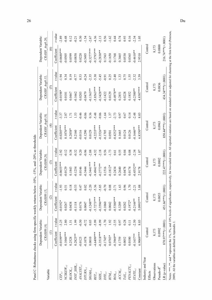
26 Du

P

anel

C: R

obus

tnes

s ch

ecks

usi

ng f

irm

-spe

cifi

c w

eekl

y re

turn

s be

low

-10

%, -

15%

, and

-20

% a

s th

resh

olds

Var

iabl

e

D

epen

dent

Var

iabl

e:

CR

ASH

0.10

t

D

epen

dent

Var

iabl

e:

CR

ASH

0.15

t

D

epen

dent

Var

iabl

e:

CR

ASH

0.20

t

D

epen

dent

Var

iabl

e:

CR

ASH

_Avg

0.10

t

D

epen

dent

Var

iabl

e:

CR

ASH

_Avg

0.15

t

D

epen

dent

Var

iabl

e:

CR

ASH

_Avg

0.20

t

(1

)

(2)

(3

)

(4)

(5

)

(6)

C

oeff

icie

nt

t-va

lue

C

oeff

icie

nt

t-va

lue

C

oeff

icie

nt

t-va

lue

C

oeff

icie

nt

t-va

lue

C

oeff

icie

nt

t-va

lue

C

oeff

icie

nt

t-va

lue

CE

Pt-

1

-0.0

199*

**

-3.2

5

-0.0

192*

-1

.93

-0

.065

5***

-2

.92

-0

.020

5***

-3

.37

-0

.019

8*

-1.9

4

-0.0

688*

**

-2.8

9

NC

SKE

Wt-

1

0.10

44**

* 2.

80

0.

0267

0.

51

-0

.012

9 -0

.12

0.

1076

***

2.87

0.01

81

0.34

-0.0

505

-0.4

8

BLO

CK

t-1

0.

2528

1.

51

0.

0438

0.

18

0.

1843

0.

38

0.

2858

* 1.

71

0.

0467

0.

19

0.

0599

0.

12

INST

_SH

Rt-

1

0.28

25**

1.

99

-0

.111

8 -0

.53

-0

.125

4 -0

.32

0.

2160

1.

53

-0

.166

2 -0

.77

-0

.085

8 -0

.21

AN

ALY

STt-

1

-0.0

125

-0.5

0

0.01

76

0.47

0.01

46

0.20

-0.0

116

-0.4

6

0.02

03

0.53

0.02

20

0.30

DTU

RN

t-1

-0

.107

8 -0

.72

0.

0047

0.

02

-0

.344

4 -0

.96

-0

.129

0 -0

.86

-0

.047

9 -0

.24

-0

.549

5 -1

.54

SIG

MA

t-1

0.

0010

0.

03

-0

.124

8**

-2.2

0

-0.3

441*

**

-2.8

8

0.01

29

0.36

-0.1

363*

* -2

.35

-0

.327

7***

-2

.67

RE

T t-1

-4.6

499*

**

-5.9

9

-5.7

273*

**

-5.3

6

-9.4

941*

**

-4.5

2

-4.2

235*

**

-5.4

8

-5.8

563*

**

-5.3

0

-9.3

793*

**

-4.3

6

SIZE

t-1

-0

.351

8***

-8

.99

-0

.359

6***

-5

.85

-0

.277

2**

-2.1

8

-0.3

526*

**

-9.0

6

-0.3

428*

**

-5.4

5

-0.2

830*

* -2

.13

DTE

t-1

-0

.174

5*

-1.7

0

-0.1

060

-0.7

0

0.15

16

0.56

-0.1

705

-1.6

4

-0.1

422

-0.9

1

0.15

63

0.56

BTM

t-1

0.

0703

* 1.

92

0.

0042

0.

08

-0

.181

2*

-1.7

3

0.05

01

1.37

0.01

29

0.25

-0.1

650

-1.6

2

RO

At-

1

-0.3

969*

* -2

.55

-0

.538

0***

-2

.71

0.

2434

0.

61

-0

.425

2***

-2

.73

-0

.497

8**

-2.4

0

0.17

68

0.44

AC

CM

t-1

0.

1759

0.

97

0.

3289

1.

63

0.

2640

0.

55

0.

1665

0.

97

0.

2851

1.

33

0.

3465

0.

74

TAX

t-1

0.

0052

0.

28

0.

0282

0.

96

0.

0478

0.

84

0.

0124

0.

67

0.

0228

0.

75

0.

0530

0.

93

PE

NA

LTY t

-1

0.

0100

0.

11

0.

1972

* 1.

70

0.

0174

0.

08

0.

0126

0.

14

0.

1852

1.

55

0.

0365

0.

16

STA

TEt-

1

-0.1

657*

* -2

.50

-0

.214

4**

-2.2

1

-0.4

552*

* -2

.34

-0

.164

6**

-2.4

8

-0.2

300*

* -2

.32

-0

.461

0**

-2.3

4

Con

stan

t

6.90

69**

* 8.

03

5.

0993

***

3.88

2.91

78

1.07

6.83

50**

* 8.

03

4.

8307

***

3.59

2.95

10

1.05

Indu

stry

and

Yea

r

Eff

ects

C

ontr

ol

C

ontr

ol

C

ontr

ol

C

ontr

ol

C

ontr

ol

C

ontr

ol

Obs

erva

tions

8,17

3

8,17

3

8,17

3

8,17

3

8,17

3

8,17

3

Pse

udo-

R2

0.

0992

0.08

53

0.

0802

0.09

63

0.

0836

0.08

00

LR

(p-

valu

e)

87

0.97

***(

<.00

01)

45

1.66

***(

<.0

001)

222.

47**

*(<

.000

1)

85

0.44

***(

<.00

01)

43

4.34

***(

<.0

001)

216.

74**

*(<.

0001

)

Not

es:

***,

**,

and

* r

epre

sent

the

1%, 5

%, a

nd 1

0% l

evel

s of

sig

nifi

canc

e, r

espe

ctiv

ely,

for

two-

tail

ed t

ests

. All

rep

orte

d t-

stat

istic

s ar

e ba

sed

on s

tand

ard

erro

rs a

djus

ted

for

clus

teri

ng a

t th

e fi

rm l

evel

(P

eter

sen,

2009

). A

ll th

e va

riab

les

are

defi

ned

in A

ppen

dix

1.

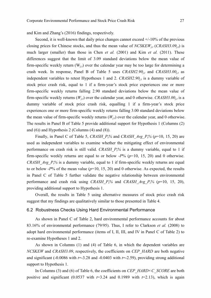
Corporate Environmental Performance and Stock Price Crash Risk 27

and Kim and Zhang’s (2016) findings, respectively.

Second, it is well-known that daily price changes cannot exceed +/-10% of the previous

closing prices for Chinese stocks, and thus the mean value of NCSKEWj,t (CRASH3.09j,t) is

much larger (smaller) than those in Chen et al. (2001) and Kim et al. (2011). These

differences suggest that the limit of 3.09 standard deviations below the mean value of

firm-specific weekly return (Wj,t) over the calendar year may be too large for determining a

crash week. In response, Panel B of Table 5 uses CRASH2.90j,t and CRASH3.00j,t as

independent variables to retest Hypotheses 1 and 2. CRASH2.90j,t is a dummy variable of

stock price crash risk, equal to 1 if a firm-year’s stock price experiences one or more

firm-specific weekly returns falling 2.90 standard deviations below the mean value of

firm-specific weekly returns (Wj,t) over the calendar year, and 0 otherwise. CRASH3.00j,t is a

dummy variable of stock price crash risk, equalling 1 if a firm-year’s stock price

experiences one or more firm-specific weekly returns falling 3.00 standard deviations below

the mean value of firm-specific weekly returns (Wj,t) over the calendar year, and 0 otherwise.

The results in Panel B of Table 5 provide additional support for Hypothesis 1 (Columns (2)

and (6)) and Hypothesis 2 (Columns (4) and (8)).

Finally, in Panel C of Table 5, CRASH_Pt% and CRASH_Avg_Pt% (p=10, 15, 20) are

used as independent variables to examine whether the mitigating effect of environmental

performance on crash risk is still valid. CRASH_Pt% is a dummy variable, equal to 1 if

firm-specific weekly returns are equal to or below -P% (p=10, 15, 20) and 0 otherwise.

CRASH_Avg_Pt% is a dummy variable, equal to 1 if firm-specific weekly returns are equal

to or below -P% of the mean value (p=10, 15, 20) and 0 otherwise. As expected, the results

in Panel C of Table 5 further validate the negative relationship between environmental

performance and crash risk using CRASH_Pt% and CRASH_Avg_Pt% (p=10, 15, 20),

providing additional support to Hypothesis 1.

Overall, the results in Table 5 using alternative measures of stock price crash risk

suggest that my findings are qualitatively similar to those presented in Table 4.

6.2 Robustness Checks Using Hard Environmental Performance

As shown in Panel C of Table 2, hard environmental performance accounts for about

83.16% of environmental performance (79/95). Thus, I refer to Clarkson et al. (2008) to

adopt hard environmental performance (items of I, II, III, and IV in Panel C of Table 2) to

re-examine Hypotheses 1 and 2.

As shown in Columns (1) and (4) of Table 6, in which the dependent variables are

NCSKEW and CRASH3.09, respectively, the coefficients on CEP_HARD are both negative

and significant (-0.0086 with t=-3.28 and -0.0403 with t=-2.59), providing strong additional

support to Hypothesis 1.

In Columns (3) and (6) of Table 6, the coefficients on CEP_HARD×C_SCORE are both

positive and significant (0.0537 with t=3.24 and 0.1989 with t=2.13), which is again

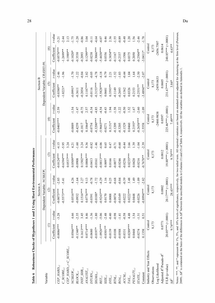
28 Du

Tab

le 6

R

obu

stn

ess

Ch

eck

s of

Hyp

oth

eses

1 a

nd

2 U

sin

g H

ard

En

viro

nm

enta

l Per

form

ance

Var

iabl

e

S

ecti

on A

Sec

tion

B

D

epen

dent

Var

iabl

e: N

CSK

EW

t

Dep

ende

nt V

aria

ble:

CR

ASH

3.09

t

(1

)

(2)

(3

)

(4)

(5

)

(6)

C

oeff

icie

nt

t-va

lue

C

oeff

icie

nt

t-va

lue

C

oeff

icie

nt

t-va

lue

C

oeff

icie

nt

t-va

lue

C

oeff

icie

nt

t-va

lue

C

oeff

icie

nt

t-va

lue

CE

P_H

AR

Dt-

1

-0.0

086*

**

-3.2

8

-0.0

075*

**

-2.8

5

-0.0

124*

**

-4.1

5

-0.0

403*

**

-2.5

9

-0.0

380*

* -2

.46

-0

.057

8***

-3

.21

C_S

CO

RE

t-1

-0.5

573*

**

-5.4

1

-0.6

394*

**

-5.9

5

-1

.022

1*

-1.9

6

-1.2

699*

* -2

.44

CE

P_H

AR

Dt-

1×C

_SC

OR

Et-

1

0.05

37**

* 3.

24

0.

1989

**

2.13

NC

SKE

Wt-

1

0.05

66**

* 4.

66

0.

0516

***

4.26

0.05

09**

* 4.

21

-0

.088

9 -1

.54

-0

.099

1*

-1.7

0

-0.1

020*

-1

.75

BL

OC

Kt-

1

-0.1

340*

* -2

.35

-0

.093

2 -1

.64

-0

.090

8 -1

.60

-0

.425

9 -1

.47

-0

.361

1 -1

.22

-0

.353

0 -1

.20

INST

_SH

Rt-

1

0.16

13**

* 3.

45

0.

1516

***

3.27

0.15

02**

* 3.

24

-0

.181

7 -0

.75

-0

.205

4 -0

.84

-0

.209

3 -0

.86

AN

ALY

STt-

1

0.07

14**

* 8.

46

0.

0776

***

9.13

0.08

06**

* 9.

36

0.

1064

**

2.57

0.11

87**

* 2.

82

0.

1299

***

3.04

DT

UR

Nt-

1

-0.0

680

-1.3

6

-0.0

391

-0.7

8

-0.0

413

-0.8

2

-0.0

754

-0.3

4

-0.0

116

-0.0

5

-0.0

238

-0.1

1

SIG

MA

t-1

-0

.019

7*

-1.8

0

-0.0

188*

-1

.72

-0

.016

1 -1

.46

-0

.320

0***

-4

.85

-0

.315

3***

-4

.78

-0

.306

6***

-4

.64

RE

Tt-

1

-1.0

926*

**

-5.0

6

-0.9

243*

**

-4.2

9

-0.8

813*

**

-4.0

6

-5.9

665*

**

-4.5

4

-5.5

828*

**

-4.1

8

-5.4

430*

**

-4.0

7

SIZ

Et-

1

-0.0

301*

* -2

.48

0.

0170

1.

16

0.

0097

0.

65

-0

.027

1 -0

.43

0.

0601

0.

79

0.

0356

0.

46

DT

Et-

1

-0.0

139

-0.4

0

0.00

88

0.25

0.01

66

0.47

0.31

51*

1.94

0.35

93**

2.

21

0.

3854

**

2.36

BT

Mt-

1

-0.0

108

-0.9

8

-0.0

074

-0.6

8

-0.0

077

-0.7

1

-0.1

209

-1.5

8

-0.1

149

-1.5

2

-0.1

167

-1.5

5

RO

At-

1

-0.0

588

-1.4

1

-0.0

349

-0.8

4

-0.0

246

-0.6

0

-0.3

205

-1.2

2

-0.2

693

-1.0

3

-0.2

337

-0.8

9

AC

CM

t-1

-0

.033

1 -0

.58

-0

.022

2 -0

.39

-0

.025

6 -0

.44

-0

.152

9 -0

.50

-0

.136

2 -0

.44

-0

.150

6 -0

.48

TA

Xt-

1

0.02

89**

* 4.

48

0.

0222

***

3.48

0.02

35**

* 3.

66

0.

0460

1.

52

0.

0326

1.

04

0.

0375

1.

20

PE

NA

LT

Yt-

1

0.04

68

1.54

0.04

48

1.49

0.04

20

1.39

0.21

93*

1.67

0.21

53

1.64

0.20

50

1.56

STA

TE

t-1

-0

.027

4 -1

.31

-0

.022

6 -1

.09

-0

.021

6 -1

.04

-0

.265

8***

-2

.60

-0

.255

1**

-2.5

0

-0.2

504*

* -2

.46

Con

stan

t

0.13

58

0.51

-0.8

994*

**

-2.8

2

-0.7

678*

* -2

.39

-1

.555

8 -1

.09

-3

.489

4**

-2.0

7

-3.0

411*

-1

.78

Indu

stry

and

Yea

r E

ffec

ts

C

ontr

ol

C

ontr

ol

C

ontr

ol

C

ontr

ol

C

ontr

ol

C

ontr

ol

Obs

erva

tion

s

8,17

3

8,17

3

8,17

3

8,17

3

8,17

3

8,17

3

Log

Lik

elih

ood

-2

460.

9838

-245

9.06

33

-2

456.

7507

Adj

uste

d R

2 /Pse

udo-

R2

0.

0771

0.08

02

0.

0812

0.05

97

0.

0605

0.06

14

F/L

R (

p-va

lue)

20.0

5***

(<

.000

1)

20

.17*

** (

<.0

001)

19.8

8***

(<

.000

1)

22

5.46

***

(<.0

001)

231.

67**

* (<

.000

1)

24

0.85

***

(<.0

001)

ΔR

2

9.74

***

28

.43*

**

9.

78**

*

7.49

***

3.

84*

4.

63**

Not

es:

***,

**,

and

* r

epre

sent

the

1%

, 5%

, and

10%

lev

els

of s

igni

fica

nce,

res

pect

ivel

y, f

or t

wo-

tail

ed t

ests

. A

ll r

epor

ted

t-st

atis

tics

are

bas

ed o

n st

anda

rd e

rror

s ad

just

ed f

or c

lust

erin

g at

the

fir

m l

evel

(P

eter

sen,

2009

). Δ

R2 i

s co

mpu

ted

on t

he b

asis

of

the

diff

eren

ces

in Δ

R2 b

etw

een

the

spec

ifie

d m

odel

s in

Col

umns

(1)

and

(5)

of

Tab

le 4

, res

pect

ivel

y. A

ll th

e va

riab

les

are

defi

ned

in A

ppen

dix

1.

Corporate Environmental Performance and Stock Price Crash Risk 29

consistent with Hypothesis 2. Both CEP_HARD and C_SCORE in Columns (3) and (6) also

have significantly negative coefficients, providing support to Hypothesis 1 and consistent

with theoretical expectations.

In a nutshell, the results in Table 6 suggest that my findings are qualitatively similar to

those presented in Table 4 after adopting hard environmental performance as the

independent variable.

VII. The Endogeneity Issue

To mitigate potential endogeneity between corporate environmental performance and

future crash risk, this study follows the literature (e.g. El Ghoul et al., 2011) to employ both

the instrumental variable approach and two-stage regression procedures.

7.1 Using the Instrumental Variable Approach to Mitigate Endogeneity

This study uses the average environmental performance of other firms in the same

industry as the instrumental variable, labelled CEP_HAT, to re-examine Hypotheses 1 and 2.

As shown in Columns (1) and (4) of Table 7, the coefficients on CEP_HAT (i.e. the fitted

values of CEP) are negative and significant (-0.0054 with t=-3.20 and -0.0284 with t=-2.69),

suggesting that the negative association between corporate environmental performance and

future crash risk is still valid after controlling for endogeneity using the instrumental

variable approach. These results also validate Hypothesis 1. In Columns (3) and (6), the

coefficients on CEP_HAT×C_SCORE are both positive and significant (0.0288 with t=2.79

and 0.0866 with t=2.23), validating Hypothesis 2 by indicating that accounting conservatism

attenuates the negative relationship between corporate environmental performance and

future crash risk.

7.2 Using Two-Stage Tobit-OLS (Logistic) Regression Procedures to Mitigate

Endogeneity

For two-stage Tobit-OLS (Logistic) regression procedures, I must identify exogenous

variables for the first stage in which corporate environmental performance (CEP) is the

dependent variable. Following Du et al. (2014), I employ eight exogenous variables as

follows: FINt-1 is the amount of equity or debt financing in year t-1 scaled by total assets at

the beginning of the year (Clarkson et al., 2008); CAPINVt-1 is the amount of capital

spending (property, plant and equipment, intangible assets and other long-term assets) in

year t-1 divided by total sales at the beginning of the year (Clarkson et al., 2008; Du et al.,

2014); LISTAGEt-1 is the number of years from a firm’s IPO; TRANSt-1 is the natural

logarithm of the total mileages of provincial highways and railways (in kilometres) in year

t-1; TAX_PROt-1 is the natural logarithm of provincial tax (in million RMB) in year t-1;

POPt-1 is the natural logarithm of the number of provincial populations in year t-1; UNVt-1 is

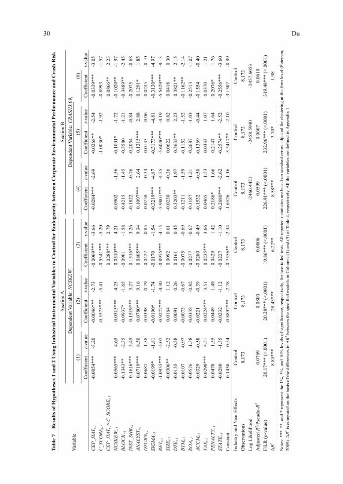
30 Du

T

able

7

Res

ult

s of

Hyp

oth

eses

1 a

nd

2 U

sin

g In

du

stri

al I

nst

rum

enta

l Var

iab

les

to C

ontr

ol f

or E

nd

ogen

eity

bet

wee

n C

orp

orat

e E

nvi

ron

men

tal P

erfo

rman

ce a

nd

Cra

sh R

isk

Var

iabl

e

S

ecti

on A

Sec

tion

B

D

epen

dent

Var

iabl

e: N

CSK

EW

t

Dep

ende

nt V

aria

ble:

CR

ASH

3.09

t

(1

)

(2)

(3

)

(4)

(5

)

(6)

C

oeff

icie

nt

t-va

lue

C

oeff

icie

nt

t-va

lue

C

oeff

icie

nt

t-va

lue

C

oeff

icie

nt

t-va

lue

C

oeff

icie

nt

t-va

lue

C

oeff

icie

nt

t-va

lue

CE

P_H

AT

t-1

-0

.005

4***

-3

.20

-0

.004

6***

-2

.73

-0

.006

9***

-3

.66

-0

.028

4***

-2

.69

-0

.026

8**

-2.5

4

-0.0

339*

**

-3.0

5

C_S

CO

RE

t-1

-0.5

573*

**

-5.4

1

-0.5

341*

**

-5.2

0

-1

.003

0*

-1.9

2

-0.8

993

-1.5

7

CE

P_H

AT

t-1×

C_S

CO

RE

t-1

0.

0288

***

2.79

0.08

66**

2.

23

NC

SKE

Wt-

1

0.05

65**

* 4.

65

0.

0515

***

4.25

0.05

10**

* 4.

21

-0

.090

2 -1

.56

-0

.100

1*

-1.7

2

-0.1

020*

* -1

.97

BL

OC

Kt-

1

-0.1

343*

* -2

.35

-0

.093

7*

-1.6

5

-0.0

901

-1.5

8

-0.4

215

-1.4

5

-0.3

580

-1.2

1

-0.3

489*

* -2

.45

INST

_SH

Rt-

1

0.16

16**

* 3.

45

0.

1519

***

3.27

0.15

16**

* 3.

26

-0

.182

2 -0

.76

-0

.205

4 -0

.84

-0

.207

5 -0

.68

AN

AL

YST

t-1

0.

0719

***

8.50

0.07

80**

* 9.

16

0.

0805

***

9.34

0.10

97**

* 2.

64

0.

1215

***

2.88

0.12

91*

1.85

DT

UR

Nt-

1

-0.0

687

-1.3

8

-0.0

398

-0.7

9

-0.0

427

-0.8

5

-0.0

758

-0.3

4

-0.0

133

-0.0

6

-0.0

245

-0.1

0

SIG

MA

t-1

-0

.019

9*

-1.8

1

-0.0

190*

-1

.74

-0

.017

0 -1

.54

-0

.321

9***

-4

.87

-0

.317

3***

-4

.81

-0

.313

0***

-4

.97

RE

Tt-

1

-1.0

955*

**

-5.0

7

-0.9

272*

**

-4.3

0

-0.8

975*

**

-4.1

5

-5.9

801*

**

-4.5

5

-5.6

040*

**

-4.1

9

-5.5

429*

**

-9.1

3

SIZ

Et-

1

-0.0

306*

* -2

.52

0.

0164

1.

12

0.

0092

0.

61

-0

.023

0 -0

.36

0.

0622

0.

82

0.

0418

0.

30

DT

Et-

1

-0.0

135

-0.3

8

0.00

91

0.26

0.01

61

0.45

0.32

03**

1.

97

0.

3635

**

2.23

0.38

21**

2.

15

BT

Mt-

1

-0.0

107

-0.9

7

-0.0

073

-0.6

7

-0.0

075

-0.6

9

-0.1

211

-1.5

9

-0.1

152

-1.5

2

-0.1

162*

* -2

.14

RO

At-

1

-0.0

576

-1.3

8

-0.0

338

-0.8

2

-0.0

277

-0.6

7

-0.3

187

-1.2

1

-0.2

687

-1.0

3

-0.2

513

-1.0

7

AC

CM

t-1

-0

.032

9 -0

.58

-0

.022

1 -0

.39

-0

.028

0 -0

.49

-0

.153

2 -0

.50

-0

.136

9 -0

.44

-0

.155

4 -0

.40

TA

Xt-

1

0.02

90**

* 4.

51

0.

0224

***

3.51

0.02

35**

* 3.

66

0.

0465

1.

53

0.

0333

1.

07

0.

0370

1.

21

PE

NA

LT

Yt-

1

0.04

70

1.55

0.04

49

1.49

0.04

29

1.42

0.21

86*

1.66

0.21

47

1.64

0.20

76*

1.76

STA

TE

t-1

-0

.028

0 -1

.35

-0

.023

2 -1

.12

-0

.022

7 -1

.10

-0

.268

0***

-2

.62

-0

.257

4**

-2.5

2

-0.2

556*

**

-3.6

0

Con

stan

t

0.14

30

0.54

-0.8

892*

**

-2.7

8

-0.7

556*

* -2

.34

-1

.652

6 -1

.16

-3

.541

7**

-2.1

0

-3.1

507

-0.9

9

Indu

stry

and

Yea

r E

ffec

ts

C

ontr

ol

C

ontr

ol

C

ontr

ol

C

ontr

ol

C

ontr

ol

C

ontr

ol

Obs

erva

tion

s

8,17

3

8,17

3

8,17

3

8,17

3

8,17

3

8,17

3

Log

Lik

elih

ood

-2

460.

4421

-245

8.59

40

-2

457.

6053

Adj

uste

d R

2 /Pse

udo-

R2

0.

0769

0.08

00

0.

0806

0.05

99

0.

0607

0.06

10

F/L

R (

p-va

lue)

20.1

7***

(<

.000

1)

20

.28*

** (

<.0

001)

19.8

6***

(<

.000

1)

22

6.91

***

(<.0

001)

232.

96**

* (<

.000

1)

31

9.48

***

(<.0

001)

ΔR

2

8.85

***

28

.43*

**

6.

22**

8.58

***

3.

70*

1.

98

Not

es:

***,

**,

and

* r

epre

sent

the

1%

, 5%

, and

10%

lev

els

of s

igni

fica

nce,

res

pect

ivel

y, f

or t

wo-

tail

ed t

ests

. A

ll r

epor

ted

t-st

atis

tics

are

bas

ed o

n st

anda

rd e

rror

s ad

just

ed f

or c

lust

erin

g at

the

fir

m l

evel

(P

eter

sen,

2009

). Δ

R2 i

s co

mpu

ted

on t

he b

asis

of

the

diff

eren

ces

in Δ

R2 b

etw

een

the

spec

ifie

d m

odel

s in

Col

umns

(1)

and

(5)

of

Tab

le 4

, res

pect

ivel

y. A

ll t

he v

aria

bles

are

def

ined

in

App

endi

x 1.

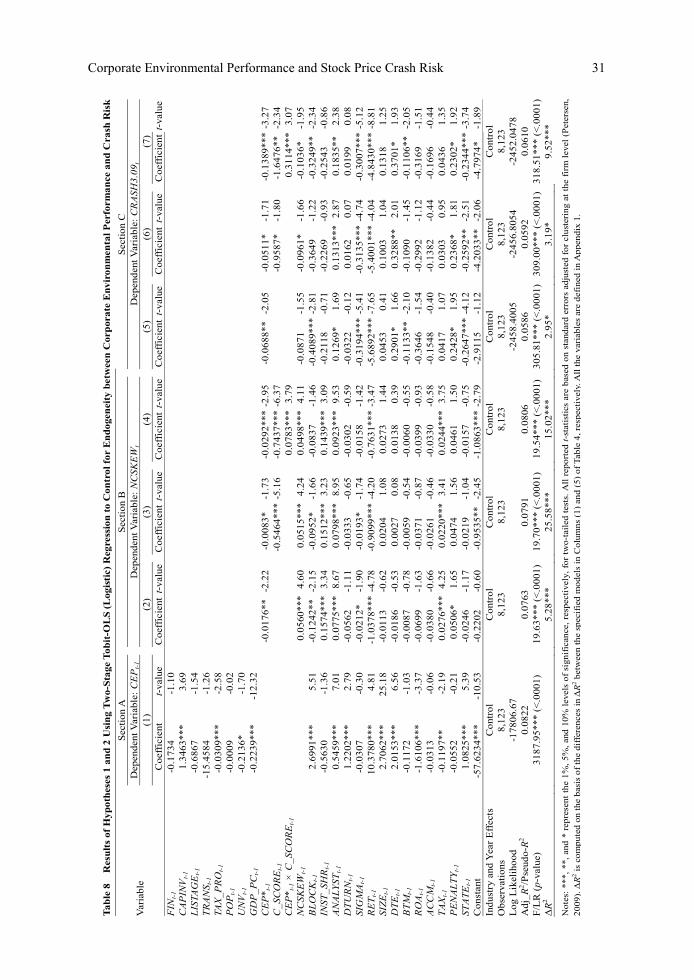
Corporate Environmental Performance and Stock Price Crash Risk 31

T

able

8

Res

ult

s of

Hyp

oth

eses

1 a

nd

2 U

sin

g T

wo-

Sta

ge T

obit

-OL

S (

Log

isti

c) R

egre

ssio

n t

o C

ontr

ol f

or E

nd

ogen

eity

bet

wee

n C

orp

orat

e E

nvi

ron

men

tal

Per

form

ance

an

d C

rash

Ris

k

Var

iabl

e

S

ecti

on A

Sec

tion

B

S

ecti

on C

Dep

ende

nt V

aria

ble:

CE

Pt-

1

D

epen

dent

Var

iabl

e: N

CSK

EW

t

Dep

end

ent V

aria

ble:

CR

ASH

3.09

t

(1)

(2

)

(3)

(4

)

(5)

(6

)

(7)

C

oeff

icie

nt

t-va

lue

C

oeff

icie

nt t

-val

ue

C

oeff

icie

nt t

-val

ue

C

oeff

icie

nt t

-val

ue

C

oef

fici

ent

t-va

lue

C

oeff

icie

nt t

-val

ue

C

oeff

icie

nt t

-val

ue

FIN

t-1

-0

.173

4 -1

.10

CA

PIN

Vt-

1

1.

3463

***

3.69

L

ISTA

GE

t-1

-0

.686

7 -1

.54

TR

AN

S t-1

-15.

4584

-1

.26

TAX

_PR

Ot-

1

-0.0

309*

**

-2.5

8

P

OP

t-1

-0

.000

9 -0

.02

UN

Vt-

1

-0

.213

6*

-1.7

0

G

DP

_PC

t-1

-0

.223

9***

-1

2.32

C

EP

* t-1

-0

.017

6**

-2.2

2

-0.0

083*

-1

.73

-0

.029

2***

-2.9

5

-0.0

688*

* -2

.05

-0

.051

1*

-1.7

1

-0.1

389*

**-3

.27

C_S

CO

RE

t-1

-0

.54

64**

*-5

.16

-0

.743

7***

-6.3

7

-0

.958

7*

-1.8

0

-1.6

476

**

-2.3

4 C

EP

* t-1

× C

_SC

OR

Et-

1

0.

0783

***

3.79

0.31

14**

*3.

07

NC

SKE

Wt-

1

0.05

60**

* 4.

60

0.

0515

***

4.24

0.04

98**

*4.

11

-0

.087

1 -1

.55

-0

.096

1*

-1.6

6

-0.1

036

* -1

.95

BL

OC

Kt-

1

2.69

91**

* 5.

51

-0

.124

2**

-2.1

5

-0.0

952*

-1

.66

-0

.083

7 -1

.46

-0

.408

9***

-2.8

1

-0.3

649

-1.2

2

-0.3

249

**

-2.3

4 IN

ST_S

HR

t-1

-0

.563

0 -1

.36

0.

1574

***

3.34

0.15

12**

*3.

23

0.

1439

***

3.09

-0.2

118

-0.7

1

-0.2

269

-0.9

3

-0.2

543

-0.8

6 A

NA

LY

STt-

1

0.

5459

***

7.01

0.07

75**

* 8.

67

0.

0798

***

8.95

0.09

23**

*9.

53

0.

1269

* 1.

69

0.

1313

***

2.87

0.18

35**

2.

38

DT

UR

Nt-

1

1.

2202

***

2.79

-0.0

562

-1.1

1

-0.0

333

-0.6

5

-0.0

302

-0.5

9

-0.0

322

-0.1

2

0.01

62

0.07

0.01

99

0.08

SI

GM

At-

1

-0.0

307

-0.3

0

-0.0

212*

-1

.90

-0

.019

3*

-1.7

4

-0.0

158

-1.4

2

-0.3

194*

**-5

.41

-0

.313

5***

-4.

74

-0

.300

7***

-5.1

2 R

ET

t-1

10

.378

0***

4.

81

-1

.037

8***

-4.

78

-0

.90

99**

*-4

.20

-0

.763

1***

-3.4

7

-5.6

892*

**-7

.65

-5

.400

1***

-4.

04

-4

.843

0***

-8.8

1 SI

ZE

t-1

2.

7062

***

25.1

8

-0.0

113

-0.6

2

0.02

04

1.08

0.02

73

1.44

0.04

53

0.41

0.10

03

1.04

0.13

18

1.25

D

TE

t-1

2.

0153

***

6.56

-0.0

186

-0.5

3

0.00

27

0.08

0.01

38

0.39

0.29

01*

1.66

0.32

88**

2.

01

0.

3701

* 1.

93

BT

Mt-

1

-0

.117

2 -1

.03

-0

.008

7 -0

.78

-0

.005

9 -0

.54

-0

.006

0 -0

.55

-0

.113

3**

-2.1

0

-0.1

090

-1.4

5

-0.1

106

**

-2.0

5 R

OA

t-1

-1

.610

6***

-3

.37

-0

.069

9 -1

.63

-0

.037

1 -0

.87

-0

.039

9 -0

.93

-0

.364

6 -1

.54

-0

.299

2 -1

.12

-0

.316

9 -1

.51

AC

CM

t-1

-0

.031

3 -0

.06

-0

.038

0 -0

.66

-0

.026

1 -0

.46

-0

.033

0 -0

.58

-0

.154

8 -0

.40

-0

.138

2 -0

.44

-0

.169

6 -0

.44

TA

Xt-

1

-0.1

197*

* -2

.19

0.

0276

***

4.25

0.02

20**

*3.

41

0.

0244

***

3.75

0.04

17

1.07

0.03

03

0.95

0.04

36

1.35

P

EN

AL

TY

t-1

-0

.055

2 -0

.21

0.

0506

* 1.

65

0.

0474

1.

56

0.

0461

1.

50

0.

2428

* 1.

95

0.

2368

* 1.

81

0.

2302

* 1.

92

STA

TE

t-1

1.

0825

***

5.39

-0.0

246

-1.1

7

-0.0

219

-1.0

4

-0.0

157

-0.7

5

-0.2

647*

**-4

.12

-0

.259

2**

-2.5

1

-0.2

344*

**-3

.74

Con

stan

t

-57.

6234

***

-10.

53

-0

.220

2 -0

.60

-0

.953

5**

-2.4

5

-1.0

863*

**-2

.79

-2

.911

5 -1

.12

-4

.203

3**

-2.0

6

-4.7

974

* -1

.89

Indu

stry

and

Yea

r E

ffec

ts

C

ont

rol

C

ontr

ol

C

ontr

ol

C

ontr

ol

C

ontr

ol

C

ontr

ol

C

ontr

ol

Obs

erva

tion

s

8,12

3

8,12

3

8,12

3

8,12

3

8,12

3

8,12

3

8,12

3 L

og L

ikel

ihoo

d

-178

06.6

7

-245

8.40

05

-2

456.

8054

-245

2.04

78

Adj

_R2 /P

seud

o-R

2

0.08

22

0.

0763

0.07

91

0.

0806

0.05

86

0.

0592

0.06

10

F/L

R (

p-va

lue)

3187

.95*

** (

<.0

001)

19.6

3***

(<

.000

1)

19

.70*

** (

<.0

001)

19.5

4***

(<

.000

1)

305

.81*

** (

<.0

001

) 3

09.0

0***

(<

.000

1)

318.

51**

* (<

.000

1)Δ

R2

5.

28**

*

25.5

8***

15.0

2***

2.95

*

3.19

*

9.52

***

Not

es:

***,

**,

and

* r

epre

sent

the

1%

, 5%

, an

d 10

% l

evel

s of

sig

nifi

canc

e, r

espe

ctiv

ely,

for

tw

o-ta

iled

tes

ts.

All

rep

orte

d t-

stat

isti

cs a

re b

ased

on

stan

dard

err

ors

adju

sted

for

clu

ster

ing

at t

he f

irm

lev

el (

Pet

erse

n,20

09).

ΔR

2 is

com

pute

d on

the

bas

is o

f th

e di

ffer

ence

s in

ΔR

2 bet

wee

n th

e sp

ecif

ied

mod

els

in C

olum

ns (

1) a

nd (

5) o

f T

able

4, r

espe

ctiv

ely.

All

the

var

iabl

es a

re d

efin

ed i

n A

ppen

dix

1.

32 Du

the percentage of provincial universities in year t-1, measured as the number of universities

in a province scaled by the total number of universities in mainland China; and GDP_PCt-1

is provincial GDP per capita (in thousand RMB) in year t-1.9

The results of the first stage, presented in Column (1) of Section A in Table 8, show

that corporate environmental performance is significantly positively associated with

BLOCKt-1, ANALYSTt-1, DTURNt-1, RETt-1, SIZEt-1, DTEt-1, STATEt-1, and CAPINVt-1, but is

significantly negatively related to ROAt-1, TAXt-1, TAX_PROt-1, UNVt-1, and GDP_PCt-1.

As shown by the results in Columns (2) and (5) of Table 8, the coefficients on CEP*

(the fitted values of CEP) are both negative and significant, suggesting a negative

association between corporate environmental performance and future crash risk, providing

significant support for Hypothesis 1. In Columns (4) and (7), the coefficients on

CEP*×C_SCORE are significantly positive, again validating Hypothesis 2. Moreover, in

Columns (4) and (7), both CEP* and C_SCORE have significantly negative coefficients,

consistent with Hypothesis 1 and the findings presented in Table 4.

7.3 Using the Propensity Score Matching Approach to Mitigate Endogeneity

Extending instrumental variables and the findings in Table 8, the propensity score

matching (PSM) approach is adopted to further address the endogeneity concern. Panel A of

Table 9 reports the results of the first stage of PSM. The full sample is partitioned into two

subsamples: a CEP_DUM subsample (CEP_DUM=1) and a non-CEP_DUM subsample

(CEP_DUM=0). CEP_DUM is an indicator variable equal to 1 if corporate environment

performance is greater than zero, and 0 otherwise. Panel A of Table 9 shows that, as

expected, CEP_DUM is significantly positively (negatively) associated with ANALYSTt-1,

RETt-1, SIZEt-1, DTEt-1, TOBINQt-1, and STATEt-1 (FINt-1 and LISTAGEt-1). Panel B of Table

9 presents univariate tests (t-tests) of differences in all variables used in the first stage of

PSM. There are significant differences in most variables between the two subsamples in the

context of the full sample. However, the differences in all variables between two

subsamples are insignificant in the matched sample, suggesting a relatively good matching

job in the first stage of PSM.

Panel C of Table 9 shows the results of retesting Hypotheses 1 and 2 using the matched

sample. Columns (2) and (6) of Panel C show significantly negative coefficients on CEPt-1,

consistent with Hypothesis 1. In addition, in Columns (4) and (8) of Panel C, positive and

significant coefficients on CEPt-1×C_SCOREt-1 further validate Hypothesis 2. Overall, Panel

C of Table 9 presents results indistinguishable from those in Table 4 (revised version) after

using the PSM approach to further address the endogeneity concern.

9 The results of the second-stage regression depend closely on the appropriateness of the instruments in the

first stage. Following Sargan (1958) and Wooldridge (1995), I conduct overidentification tests, and find that Sargan χ2 statistics and Wooldridge χ2 statistics are both insignificant, suggesting that there is no serious overidentification in the first-stage regression.

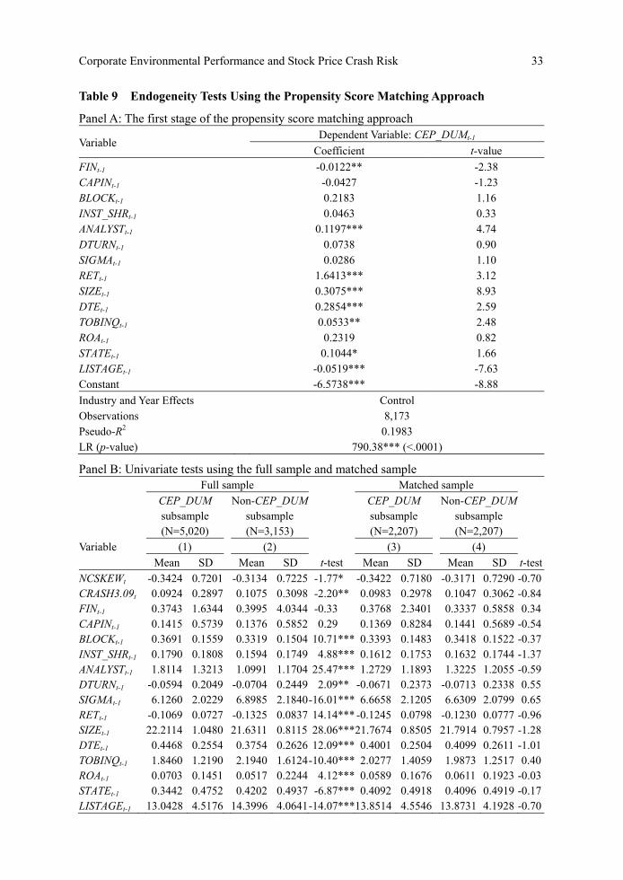
Corporate Environmental Performance and Stock Price Crash Risk 33

Table 9 Endogeneity Tests Using the Propensity Score Matching Approach

Panel A: The first stage of the propensity score matching approach

Variable Dependent Variable: CEP_DUMt-1

Coefficient t-value

FINt-1 -0.0122** -2.38 CAPINt-1 -0.0427 -1.23 BLOCKt-1 0.2183 1.16 INST_SHRt-1 0.0463 0.33 ANALYSTt-1 0.1197*** 4.74 DTURNt-1 0.0738 0.90 SIGMAt-1 0.0286 1.10 RETt-1 1.6413*** 3.12 SIZEt-1 0.3075*** 8.93 DTEt-1 0.2854*** 2.59 TOBINQt-1 0.0533** 2.48 ROAt-1 0.2319 0.82 STATEt-1 0.1044* 1.66 LISTAGEt-1 -0.0519*** -7.63 Constant -6.5738*** -8.88

Industry and Year Effects Control Observations 8,173 Pseudo-R2 0.1983 LR (p-value) 790.38*** (<.0001)

Panel B: Univariate tests using the full sample and matched sample Full sample Matched sample

CEP_DUM subsample (N=5,020)

Non-CEP_DUM

subsample (N=3,153)

CEP_DUM subsample (N=2,207)

Non-CEP_DUM subsample (N=2,207)

Variable (1) (2) (3) (4)

Mean SD Mean SD t-test Mean SD Mean SD t-test

NCSKEWt -0.3424 0.7201 -0.3134 0.7225 -1.77* -0.3422 0.7180 -0.3171 0.7290 -0.70 CRASH3.09t 0.0924 0.2897 0.1075 0.3098 -2.20** 0.0983 0.2978 0.1047 0.3062 -0.84 FINt-1 0.3743 1.6344 0.3995 4.0344 -0.33 0.3768 2.3401 0.3337 0.5858 0.34 CAPINt-1 0.1415 0.5739 0.1376 0.5852 0.29 0.1369 0.8284 0.1441 0.5689 -0.54 BLOCKt-1 0.3691 0.1559 0.3319 0.1504 10.71*** 0.3393 0.1483 0.3418 0.1522 -0.37 INST_SHRt-1 0.1790 0.1808 0.1594 0.1749 4.88*** 0.1612 0.1753 0.1632 0.1744 -1.37 ANALYSTt-1 1.8114 1.3213 1.0991 1.1704 25.47*** 1.2729 1.1893 1.3225 1.2055 -0.59 DTURNt-1 -0.0594 0.2049 -0.0704 0.2449 2.09** -0.0671 0.2373 -0.0713 0.2338 0.55 SIGMAt-1 6.1260 2.0229 6.8985 2.1840-16.01*** 6.6658 2.1205 6.6309 2.0799 0.65 RETt-1 -0.1069 0.0727 -0.1325 0.0837 14.14*** -0.1245 0.0798 -0.1230 0.0777 -0.96 SIZEt-1 22.2114 1.0480 21.6311 0.8115 28.06***21.7674 0.8505 21.7914 0.7957 -1.28 DTEt-1 0.4468 0.2554 0.3754 0.2626 12.09*** 0.4001 0.2504 0.4099 0.2611 -1.01 TOBINQt-1 1.8460 1.2190 2.1940 1.6124-10.40*** 2.0277 1.4059 1.9873 1.2517 0.40 ROAt-1 0.0703 0.1451 0.0517 0.2244 4.12*** 0.0589 0.1676 0.0611 0.1923 -0.03 STATEt-1 0.3442 0.4752 0.4202 0.4937 -6.87*** 0.4092 0.4918 0.4096 0.4919 -0.17 LISTAGEt-1 13.0428 4.5176 14.3996 4.0641-14.07***13.8514 4.5546 13.8731 4.1928 -0.70

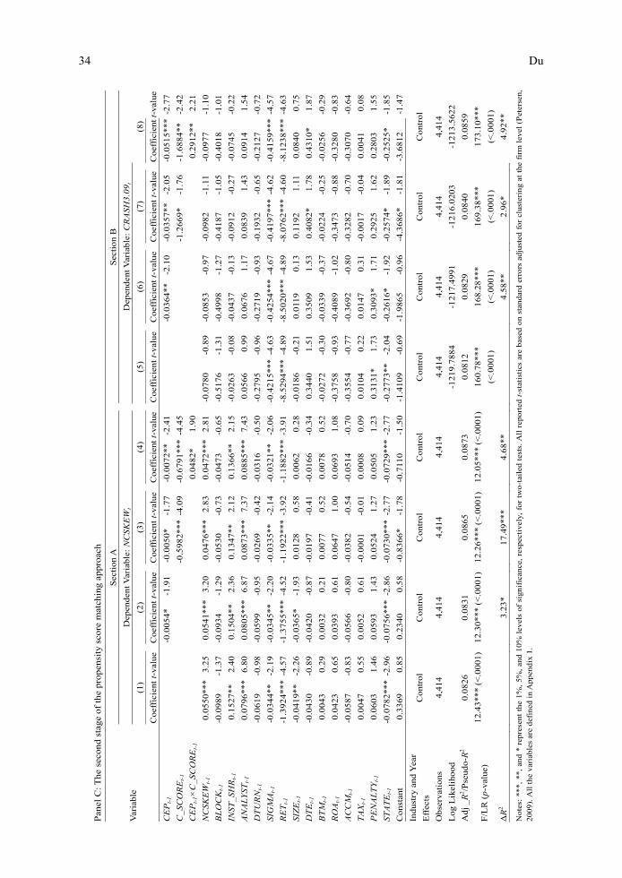
34 Du

Pan

el C

: The

sec

ond

stag

e of

th

e pr

open

sity

sco

re m

atch

ing

appr

oach

Var

iab

le

S

ecti

on A

Sec

tio

n B

D

epen

den

t V

aria

ble:

NC

SK

EW

t

Dep

end

ent

Var

iabl

e: C

RA

SH

3.0

9t

(1

)

(2)

(3

)

(4)

(5

)

(6)

(7

)

(8)

C

oeff

icie

nt t

-val

ue

Coe

ffic

ient

t-v

alue

C

oeff

icie

nt t

-val

ue

Coe

ffic

ient

t-v

alue

C

oeff

icie

nt t

-val

ue

Coe

ffic

ient

t-v

alue

C

oeff

icie

nt t

-val

ue

Co

effi

cien

t t-

valu

e

CE

Pt-

1

-0.0

05

4*

-1.9

1

-0

.00

50

* -1

.77

-0.0

07

2**

-2

.41

-0

.03

64

**

-2.1

0

-0

.03

57

**

-2.0

5

-0

.05

15

***

-2.7

7

C_

SC

OR

Et-

1

-0

.59

82

***

-4

.09

-

0.6

79

1**

*-4

.45

-1.2

66

9*

-1.7

6

-1

.68

84

**

-2.4

2

CE

Pt-

1×

C_S

CO

RE

t-1

0.0

482

* 1

.90

0.2

912

**

2.2

1

NC

SK

EW

t-1

0

.05

50**

*3

.25

0

.05

41**

*3

.20

0

.04

76**

*

2.8

3

0.0

472

***

2.8

1

-0.0

78

0 -0

.89

-0.0

85

3 -0

.97

-0.0

98

2 -1

.11

-0.0

97

7 -1

.10

BL

OC

Kt-

1

-0

.09

89

-1.3

7

-0

.09

34

-1.2

9

-0

.05

30

-0.7

3

-0

.04

73

-0.6

5

-0

.51

76

-1.3

1

-0

.49

98

-1.2

7

-0

.41

87

-1.0

5

-0

.40

18

-1.0

1

INS

T_

SH

Rt-

1

0.1

527

**

2.4

0

0.1

504

**

2.3

6

0.1

347

**

2.1

2

0.1

366

**

2.1

5

-0.0

26

3 -0

.08

-0.0

43

7 -0

.13

-0.0

91

2 -0

.27

-0.0

74

5 -0

.22

AN

AL

YS

Tt-

1

0

.07

96**

*6

.80

0

.08

05**

*6

.87

0

.08

73**

*

7.3

7

0.0

885

***

7.4

3

0.0

566

0

.99

0

.06

76

1.1

7

0.0

839

1

.43

0

.09

14

1.5

4

DT

UR

Nt-

1

-0

.06

19

-0.9

8

-0

.05

99

-0.9

5

-0

.02

69

-0.4

2

-0

.03

16

-0.5

0

-0

.27

95

-0.9

6

-0

.27

19

-0.9

3

-0

.19

32

-0.6

5

-0

.21

27

-0.7

2

SIG

MA

t-1

-0

.03

44

**

-2.1

9

-0

.03

45

**

-2.2

0

-0

.03

35

**

-2.1

4

-0

.03

21

**

-2.0

6

-0

.42

15

***

-4.6

3

-0

.42

54

***

-4

.67

-

0.4

19

7**

* -

4.6

2

-0

.41

59

***

-4.5

7

RE

Tt-

1

-1.3

92

4**

*-4

.57

-

1.3

75

5**

*-4

.52

-

1.1

92

2**

* -

3.9

2

-1

.18

82

***

-3.9

1

-8

.52

94

***

-4.8

9

-8

.50

20

***

-4

.89

-

8.0

76

2**

* -

4.6

0

-8

.12

38

***

-4.6

3

SIZ

Et-

1

-0.0

41

9**

-2

.26

-0.0

36

5*

-1.9

3

0

.01

28

0.5

8

0.0

062

0

.28

-0

.01

86

-0.2

1

0

.011

9 0

.13

0

.119

2 1

.11

0

.08

40

0.7

5

DT

Et-

1

-0

.04

30

-0.8

9

-0

.04

20

-0.8

7

-0

.01

97

-0.4

1

-0

.01

66

-0.3

4

0

.34

40

1.5

1

0.3

509

1

.53

0

.40

82*

1.7

8

0.4

310

* 1

.87

BT

Mt-

1

0

.00

43

0.2

9

0.0

032

0

.21

0

.00

77

0.5

2

0.0

078

0

.52

-0

.02

72

-0.3

0

-0

.03

39

-0.3

7

-0

.02

24

-0.2

5

-0

.02

56

-0.2

9

RO

At-

1

0

.04

23

0.6

5

0.0

393

0

.61

0

.06

47

1.0

0

0.0

693

1

.08

-0

.37

58

-0.9

3

-0

.40

89

-1.0

2

-0

.34

73

-0.8

8

-0

.32

80

-0.8

3

AC

CM

t-1

-0

.05

87

-0.8

3

-0

.05

66

-0.8

0

-0

.03

82

-0.5

4

-0

.05

14

-0.7

0

-0

.35

54

-0.7

7

-0

.36

92

-0.8

0

-0

.32

82

-0.7

0

-0

.30

70

-0.6

4

TA

Xt-

1

0.0

047

0

.55

0

.00

52

0.6

1

-0.0

00

1 -0

.01

0.0

008

0

.09

0

.01

04

0.2

2

0.0

147

0

.31

-0

.00

17

-0.0

4

0

.00

41

0.0

8

PE

NA

LT

Yt-

1

0

.06

03

1.4

6

0.0

593

1

.43

0

.05

24

1.2

7

0.0

505

1

.23

0

.31

31*

1.7

3

0.3

093

* 1

.71

0

.29

25

1.6

2

0.2

803

1

.55

ST

AT

Et-

1

-0

.07

82

***

-2.9

6

-0

.07

56

***

-2.8

6

-0

.07

30

***

-2

.77

-

0.0

72

9**

*-2

.77

-0.2

77

3**

-2

.04

-0.2

61

6*

-1.9

2

-0

.25

74

* -1

.89

-0.2

52

5*

-1.8

5

Co

nsta

nt

0

.33

69

0.8

5

0.2

340

0

.58

-0

.83

66

* -1

.78

-0.7

110

-1.5

0

-1

.41

09

-0.6

9

-1

.98

65

-0.9

6

-4

.36

86

* -1

.81

-3.6

81

2 -1

.47

Ind

ustr

y an

d Y

ear

Eff

ects

C

ont

rol

C

ont

rol

C

ont

rol

C

ont

rol

C

ont

rol

C

ont

rol

C

ont

rol

C

ont

rol

Ob

serv

atio

ns

4

,41

4

4,4

14

4

,41

4

4,4

14

4

,41

4

4,4

14

4

,41

4

4,4

14

Lo

g L

ikel

iho

od

-12

19

.788

4

-12

17

.499

1

-12

16

.020

3

-12

13

.562

2

Ad

j _

R2 /P

seud

o-R

2

0.0

826

0.0

831

0.0

865

0.0

873

0.0

812

0.0

829

0.0

840

0.0

859

F/L

R (

p-v

alue

)

12

.43

***

(<.0

00

1)

12.

30

***

(<.0

00

1)

12

.26

***

(<.0

00

1)

12

.05

***

(<.0

00

1)

1

60

.78

***

(<.0

001

)

1

68

.28

***

(<.0

001

)

1

69

.38

***

(<.0

001

)

1

73

.10

***

(<.0

001

)

ΔR

2

3

.23

*

17

.49

***

4.6

8**

4.5

8**

2.9

6*

4

.92

**

Not

es:

***,

**,

an

d *

rep

rese

nt t

he 1

%,

5%,

and

10%

lev

els

of s

ign

ific

ance

, re

spec

tive

ly,

for

two-

tail

ed t

ests

. A

ll r

epo

rted

t-s

tati

stic

s ar

e b

ased

on

sta

ndar

d er

rors

adj

uste

d fo

r cl

ust

erin

g at

th

e fi

rm l

evel

(P

eter

sen,

2009

). A

ll t

he

vari

able

s ar

e d

efin

ed i

n A

ppen

dix

1.

Corporate Environmental Performance and Stock Price Crash Risk 35

VIII. Conclusion, Managerial Implications, and Limitations

This study examines the influence of corporate environmental performance on stock

price crash risk and further investigates the interactive effect between environmental

performance and accounting conservatism on stock price crash risk. Using a sample of

Chinese listed firms, this study finds a negative relationship between environmental

performance and future crash risk, as well as substitutive effects between environmental

performance and accounting conservatism on mitigating crash risk.

My findings also have several managerial implications. First, it motivates two branches

of future research: (1) the association between corporate environmental performance and

stock market reactions and (2) market efficiency in incorporating and identifying

environmental reputation as an intangible asset. Stock price crash risk can be viewed as a

special and negative market reaction to bad news hoarding (Hanlon and Slemrod, 2009).

Because environmentally responsible firms can attract environmentally sensitive

stakeholders, firms with better environmental performance can distinguish themselves from

their counterparts, and thus the impact of corporate environmental performance on stock

market reactions and market efficiency is worthy of further research.

Second, this study suggests that environmentally responsible firms face fewer future

price crashes due to their reputation, fewer future risks, managers’ better moral integrity, and

greater information transparency. Thus, environmental performance can be viewed as an

important conduit for communicating “soft information” and managers’ moral integrity to

the market. Environmentally friendly firms can actually shape their reputation and build

positive moral capital, thus mitigating future crash risk. In this regard, my study identifies a

specific benefit of corporate environmental performance.

Finally, my study reveals that accounting conservatism mitigates future crash risk and

validates the moderating effect of accounting conservatism. These findings can motivate

future studies to further focus on other characteristics of accounting information and

examine their impacts on stock price crash risk. More importantly, this study shows that

accounting conservatism weakens the negative effect of environmental performance on

future crash risk, suggesting that accounting information and business ethics can substitute

each other in affecting corporate behaviour.

Of course, this study has its limitations. First, due to the fact that there is as yet no CSR

database in China, I follow GRI (2006) and Clarkson et al. (2008) to hand-collect data on

environmental performance. As suggested by Rahman and Post (2012), it would be better to

construct a multidimensional measure of environmental performance, and then address its

influence on future crash risk and other financial behaviour. Second, due to data limitations,

my sample covers only six years, a relatively short period, and thus my findings need

validation by additional examinations based on longer sample periods. Finally, this study is

conducted in the context of China, and thus my findings may not be generalisable to

36 Du

developed markets. Future research can further address the influence of corporate

environmental performance on stock price crash risk in international settings.

As a logical extension of this study, researchers should distinguish CSR strengths

from CSR weaknesses to address whether these have similar or asymmetric impacts on

future crash risk and other corporate financial behaviours. Moreover, it would be very

interesting for researchers to examine how different CSR dimensions and accounting

information jointly impact corporate financial behaviours.

“Open Access. This article is distributed under the terms of the Creative Commons Attribution License which permits any use, distribution, and reproduction in any medium,

provided the original author(s) and the source are credited.”

References

Al-Tuwaijri, S. A., Christensen, T. E., and Hughes, K. E. (2004), ‘The relations among

environmental disclosure, environmental performance, and economic performance: A

simultaneous equations approach’, Accounting, Organizations and Society 29 (5-6):

447-471.

Basu, S. (1997), ‘The conservatism principle and asymmetric timeliness of earnings’,

Journal of Accounting and Economics 24 (1): 3-37.

Beaulieu, P. R. (2001), ‘The effects of judgments of new clients’ integrity upon risk

judgments, audit evidence and fees’, Auditing: A Journal of Practices and Theory 20

(2): 85-100.

Cai, L. and He, C. (2014), ‘Corporate Environmental Responsibility and Equity Prices’,

Journal of Business Ethics 125 (4): 617-635.

Chen, J. C., Patten, D. M., and Roberts, R. W. (2008), ‘Corporate charitable contributions: A

corporate social performance or legitimacy strategy?’, Journal of Business Ethics 82

(1): 131-144.

Chen, J., Chan, K. C., Dong, W., and Zhang, F. (2017), ‘Internal control and stock price

crash risk: Evidence from China’, European Accounting Review 26 (1): 125-152.

Chen, J., Hong, H., and Stein, J. (2001), ‘Forecasting crashes: Trading volume, past returns,

and conditional skewness in stock prices’, Journal of Financial Economics 61 (3):

345-381.

Clarkson, P. M., Li, Y., Richardson, G. D., and Vasvari, F. P. (2008), ‘Revisiting the relation

between environmental performance and environmental disclosure: An empirical

analysis’, Accounting, Organizations and Society 33 (4): 303-327.

Cohen, M. A., Fenn, S. A., and Konar, S. (1997), ‘Environmental and financial performance:

Are they related?’, Working Paper, Owen Graduate School of Management, Nashville,

Corporate Environmental Performance and Stock Price Crash Risk 37

TN.

Costello, A. M. and Wittenberg-Moerman, R. (2011), ‘The Impact of Financial Reporting

Quality on Debt Contracting: Evidence from Internal Control Weakness Reports’,

Journal of Accounting Research 49 (1): 97-136.

Cormier, D., Gordon, I. M., and Magnan, M. (2004), ‘Corporate environmental disclosure:

Contrasting management’s perceptions with reality’, Journal of Business Ethics 49 (2):

143-165.

Cormier, D. and Magnan, M. (1999), ‘Corporate environmental disclosure strategies:

Determinants, costs and benefits’, Journal of Accounting, Auditing and Finance 14 (3):

429-451.

Cui J., Jo, H., and Li, Y. (2015), ‘Corporate social responsibility and insider trading’,

Journal of Business Ethics 130 (4): 869-887.

Deegan, C. and Gordon, B. (1996), ‘A study of the environmental disclosure practices of

Australian corporations’, Accounting and Business Research 26 (3): 187-199.

DeFond, M. L., Lim, C. Y., and Zang, Y. (2016), ‘Client Conservatism and Auditor-Client

Contracting’, The Accounting Review 91 (1): 69-98.

Deng, X., Kang, J., and Low, B. S. (2013), ‘Corporate social responsibility and shareholder

value maximization: Evidence from mergers’, Journal of Financial Economics 110 (1):

87-109.

Dhaliwal, D. S., Li, O. Z., Tsang, A., and Yang, Y. G. (2011), ‘Voluntary nonfinancial

disclosure and the cost of equity capital: The initiation of corporate social

responsibility reporting’, The Accounting Review 86 (1): 59-100.

Dhaliwal, D. S., Radhakrishnan, S., Tsang, A., and Yang, Y. G. (2012), ‘Nonfinancial

disclosure and analyst forecast accuracy: International evidence on corporate social

responsibility disclosure’, The Accounting Review 87 (3): 723-759.

Dixon-Fowler, H. R., Slater, D. J., Johnson, J. L., Ellstrand, A. E., and Romi, A. M. (2013),

‘Beyond “does it pay to be green?” A meta-analysis of moderations of CEP-CFP

relationship’, Journal of Business Ethics 112 (2): 353-366.

Du, X. (2015a), ‘How the market value greenwashing? Evidence from China’, Journal of

Business Ethics 128 (3): 547-574.

Du, X. (2015b), ‘Is corporate philanthropy used as environmental misconduct dressing?

Evidence from Chinese family-owned firms’, Journal of Business Ethics 129 (2):

341-361.

Du, X., Jian, W., Zeng, Q., and Du, Y. (2014), ‘Corporate Environmental Responsibility in

Polluting Industries: Does Religion Matter?’, Journal of Business Ethics 124 (3):

485-507.

Du, X., Weng, J., Zeng, Q., Chang, Y., and Pei, H. (2017), ‘Do lenders applaud corporate

environmental performance? Evidence from Chinese private-owned Firms’, Journal of

38 Du

Business Ethics 143 (1): 179-207.

El Ghoul, S., Guedhami, O., Kwok, C., and Mishra, D. (2011), ‘Does corporate social

responsibility affect the cost of capital?’, Journal of Banking and Finance 35 (9):

2388-2406.

Ettredge, M., Huang, Y., and Zhang, W. (2012), ‘Earnings restatements and differential

timeliness of accounting conservatism’, Journal of Accounting and Economics 53 (3):

489-503.

Giuli, A. D. and Kostovetsky, L. (2014), ‘Are red or blue companies more likely to go green?

Politics and corporate social responsibility’, Journal of Financial Economics 111 (1):

158-180.

Global Reporting Initiative (2006), Sustainability Reporting Guidelines, retrieved 22 June

2014, available at: www.globalreporting.org.

Gray, R., Kouhy R., and Lavers, S. (1995), ‘Corporate social and environmental reporting: A

review of the literature and a longitudinal study of UK disclosure’, Accounting,

Auditing and Accountability Journal 8 (2): 47-77.

Guenster, N., Bauer, R., Derwall, J., and Koedijk, K. (2010), ‘The economic value of

corporate co-efficiency’, European Financial Management 17 (4): 679-704.

Guthrie, J. and Parker, L. (1989), ‘Corporate social reporting: A rebuttal of legitimacy

theory’, Accounting and Business Research 19 (76): 343-352.

Hanlon, M. and Slemrod, J. (2009), ‘What does tax aggressiveness signal? Evidence from

stock price reactions to news about tax shelter involvement’, Journal of Public

Economics 93 (1-2): 126-141.

Heflin, F., Hsu, C., and Jin, Q. (2015), ‘Accounting conservatism and street earnings’,

Review of Accounting Studies 20 (2): 674-709.

Heyes, A. G. (1996), ‘Lender penalty for environmental damage and the equilibrium cost of

capital’, Economica 63 (250): 311- 323.

Hutton, A. P., Marcus, A. J., and Tehranian, H. (2009), ‘Opaque financial reports, R2, and

crash risk’, Journal of Financial Economics 94 (1): 67-86.

Ilinitch, A. Y., Soderstrom, N. S., and Thomas, T. E. (1998), ‘Measuring corporate

environmental performance’, Journal of Accounting and Public Policy 17 (4-5):

383-408.

Ingram, R. and Frazier, K. B. (1980), ‘Environmental performance and corporate disclosure’,

Journal of Accounting Research 18 (2): 614-622.

Keiso, D. E., Weygandt, J. J., and Warfield, T. D. (2007), Intermediate Accounting (12th

Edition), John Wiley & Sons.

Khan, M. and Watts, R. (2009), ‘Estimation and empirical properties of a firm-year measure

of accounting conservatism’, Journal of Accounting and Economics 48 (2): 132-150.

Kim, J. B., Li, Y., and Zhang, L. (2011), ‘Corporate tax avoidance and stock price crash risk:

Corporate Environmental Performance and Stock Price Crash Risk 39

Firm-level analysis’, Journal of Financial Economics 100 (3): 639-662.

Kim, Y., Park, M. S., and Wier, B. (2012), ‘Is earnings quality associated with corporate

social responsibility?’, The Accounting Review 87 (3): 761-796.

Kim, J. B. and Zhang, L. (2016), ‘Accounting conservatism and stock price crash risk:

Firm-level evidence’, Contemporary Accounting Research 33 (1): 412-441.

Kim, Y., Li, H., and Li, S. (2014), ‘Corporate social responsibility and stock price crash risk.

Journal of Banking and Finance 43: 1-13.

Koehn, D. and Ueng, J. (2010), ‘Is philanthropy used by corporate wrongdoers to buy good

will?’, Journal of Management and Governance 14 (1): 1-16.

Konar, S. and Cohen, M. A. (2001), ‘Does the market value environmental performance?’,

Review of Economics and Statistics 83 (2): 281-289.

Lanis, R. and Richardson, G. (2012), ‘Corporate social responsibility and tax aggressiveness:

An empirical analysis’, Journal of Accounting and Public Policy 31 (1): 86-108.

Meng, X. H., Zeng, S. X., Tam, C. M., and Xu, X. D. (2013), ‘Whether top executives’

turnover influences environmental responsibility: From the perspective of

environmental information disclosure’, Journal of Business Ethics 114 (2): 341-353.

Murphy, C. J. (2002), ‘The profitable correlation between environmental and financial

performance: A review of the research’, Light Green Advisors Inc.: Seattle, WA.

Orlitzky, M., Schmidt, F. L., and Rynes, S. L. (2003), ‘Corporate social and financial

performance: A meta-analysis’, Organization Studies 24 (3): 403-441.

Paillé, P., Chen, Y., Boiral, O., and Jin, J. (2014), ‘The impact of human resource

management on environmental performance: An employee-level study’, Journal of

Business Ethics 121 (3): 451-466.

Patten, D. M. (1992), ‘Intra-industry environmental disclosures in response to the Alaskan

oil spill’, Accounting, Organizations and Society 17 (5): 471-475.

Petersen, M. A. (2004), ‘Information: Hard and soft’, Working Paper, Kellogg School of

Management, Northwest University.

Petersen, M. A. (2009), ‘Estimating standard errors in finance panel data sets: Comparing

approaches’, Review of Financial Studies 22 (1): 435-480.

Petersen, M. A. and Rajan, R. G. (1994), ‘The benefits of lending relationships: Evidence

from small business data’, The Journal of Finance 49 (1): 3-37.

Rahman, N. and Post, C. (2012), ‘Measurement issues in environmental corporate social

responsibility (ECSR): Toward a transparent, reliable, and construct valid instrument’,

Journal of Business Ethics 105 (3): 307-319.

Russo, M. V. and Fouts, P. A. (1997), ‘A resource-based perspective on corporate

environmental performance and profitability’, Academy of Management Journal 40 (3):

534-559.

Sargan, J. D. (1958), ‘The estimation of economic relationships using instrumental variables.

40 Du

Econometrica 26 (3): 393-415.

Sharfman, M. P. and Fernando, C. S. (2008), ‘Environmental risk management and the cost

of capital’, Strategic Management Journal 29 (6): 569-592.

Siegel, D. S. and Vitaliano, D. F. (2007), ‘An empirical analysis of the strategic use of

corporate social responsibility’, Journal of Economics and Management Strategy 16

(3): 773-792.

Toms, J. S. (2002), ‘Firm resources, quality signals and the determinants of corporate

environmental reputation: Some UK evidence’, The British Accounting Review 34 (3):

257-282.

Walker, K., Ni, N., and Huo, W. (2013), ‘Is the red dragon green? An examination of the

antecedents and consequences of environmental proactivity in China’, Journal of

Business Ethics 125 (1): 27-43.

Wiseman, J. (1982), ‘An evaluation of environmental disclosures made in corporate annual

reports’, Accounting, Organizations and Society 7 (1): 53-63.

Wooldridge, J. M. (1995), ‘Score diagnostics for linear models estimated by two stage least

squares’, in Maddala, G. S., Srinivasan, T. N., and Phillips, P. C. B. (eds), Advances in

Econometrics and Quantitative Economics: Essays in Honor of Professor C. R. Rao,

Oxford: Blackwell, pp. 66-87.

Xu, N., Li, X., Yuan, Q., and Chan, K. C. (2014), ‘Excess perks and stock price crash risk:

Evidence from China’, Journal of Corporate Finance 25: 419-434.

Xu, N., Jiang, X., Chan, K. C., and Yi, Z. (2013), ‘Analyst coverage, optimism, and stock

price crash risk: Evidence from China’, Pacific-Basin Finance Journal 25: 217-239.

Zhang, M., Xie, L., and Xu, H. (2016), ‘Corporate philanthropy and stock price crash risk:

Evidence from China’, Journal of Business Ethics 139 (3): 595-617.

Zyglidopoulos, S. C., Georgiadis, A. P., Carroll, C. E., and Siegel, D. S. (2012), ‘Does

media attention drive corporate social responsibility?’, Journal of Business Research

65 (11): 1622-1627.

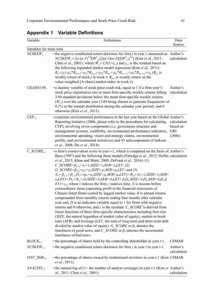
Corporate Environmental Performance and Stock Price Crash Risk 41

Appendix 1 Variable Definitions

Variable Definitions Data Source

Variables for main tests NCSKEWt = the negative conditional return skewness for firm j in year t, measured as

NCSKEWj,t=-[n (n-1)3/2ΣW3j,t]/[(n-1)(n-2)(ΣW2

j,t)3/2] (Kim et al., 2011;

Chen et al., 2001), where Wj,t=LN(1+εj,t) and εj,t is the residual based on the following expanded market model regression (Kim et al., 2011): Rj,τ=μj+μ1j*Rm,τ-2+μ2j*Rm,τ-1+μ3j*Rm,τ+μ4j*Rm, τ+1+μ5j*Rm, τ+2+εjτ (Rj,τ is weekly return of stock j in week τ; Rm,τ is weekly return on the value-weighted [A-share] market index in week τ).

Author’s calculation

CRASH3.09t = a dummy variable of stock price crash risk, equal to 1 if a firm-year’s stock price experiences one or more firm-specific weekly returns falling 3.09 standard deviations below the mean firm-specific weekly returns (Wj,t) over the calendar year (3.09 being chosen to generate frequencies of 0.1% in the normal distribution during the calendar year period), and 0 otherwise (Kim et al., 2011).

Author’s calculation

CEPt-1 = corporate environmental performance in the last year based on the Global Reporting Initiative (2006, please refer to the procedures for calculating CEP), involving seven components (i.e. governance structure and management systems, credibility, environmental performance indicators, environmental spending, vision and strategy claims, environmental profile, and environmental initiatives) and 45 subcomponents (Clarkson et al., 2008; Du et al., 2014).

Author’s calculation based on GRI (2006)

C_SCOREt-1 = a firm’s conservatism score in year t-1, which is computed on the basis of Basu (1997) and the following three models (Ettredge et al., 2012; Heflin et al., 2015; Khan and Watts, 2009; DeFond et al., 2016): (1) C_SCORE=β4,i,t=λ1+λ2SIZE+λ3M/B+λ4LEV, (2) G_SCORE=β3,i,t=μ1+μ2SIZE+μ3M/B+μ4LEV, and (3) Xi,t=β1,i,t+β2,i,tDi,t+(μ1+μ2SIZE+μ3M/B+μ4LEV)×Ri,t+(λ1+λ2SIZE+λ3M/B+λ4LEV)×Di,t×Ri,t+(δ1SIZE+δ2M/B+δ3LEV+δ4Di,tSIZE+δ5Di,tM/B+δ6Di,tLEV)+εi,t, where i indexes the firm, t indexes time, X is income before extraordinary items (operating profit in the financial statements of Chinese listed firms) scaled by lagged market value, R is annual returns compounded from monthly returns ending four months after calendar year end, D is an indicator variable equal to 1 for firms with negative returns and 0 otherwise, and ε is the residual. C_SCORE is derived from linear functions of three firm-specific characteristics including firm size (SIZE, the natural logarithm of market value of equity), market-to-book ratio (M/B), and leverage (LEV, the sum of long-term and short-term debt divided by market value of equity). G_SCORE or β3 denotes the timeliness of good news, and C_SCORE or β4 denotes the incremental timeliness of bad news.

Author’s calculation

BLOCKt-1 = the percentage of shares held by the controlling shareholder in year t-1. CSMAR

NCSKEWt-1 = the negative conditional return skewness for firm j in year t in year t-1. Author’s calculation

INST_SHRt-1 = the percentage of shares owned by institutional investors in year t-1 (Kim et al., 2011).

CSMAR

ANALYSTt-1 = the natural log of (1+ the number of analyst coverage) in year t-1 (Kim et al., 2011; Chen et al., 2001).

Author’s calculation

42 Du

DTURNt-1 = average monthly share turnover over the current calendar year period minus the average monthly share turnover over the previous calendar year period (monthly share turnover is calculated as the monthly trading volume divided by the total number of shares outstanding during the month) (Chen et al., 2001).

Author’s calculation based on CSMAR

SIGMAt-1 = the standard deviation of firm-specific weekly returns over the calendar year period t-1 (multiplied by 100) (Kim et al., 2011).

Author’s calculation

RETt-1 = the arithmetic average of firm-specific weekly returns in year t-1 (multiplied by 100) (Kim et al., 2011).

Author’s calculation

SIZEt-1 = the natural logarithm of the market value of equity at the end of year t-1 (Kim et al., 2011).

Author’s calculation

DTEt-1 = the lagged ratio of total liabilities at the end of year t-1 to the market value of equity at the end of year t-1.

CSMAR

BTMt-1 = the lagged ratio of book-to-market, measured as book value scaled by the market value of equity at the end of year t-1 (Kim et al., 2011; Chen et al., 2001).

CSMAR

ROAt-1 = returns on total assets in year t-1, measured as income before extraordinary items divided by lagged total assets (Kim et al., 2011).

CSMAR

ACCMt-1 = the extent of discretionary accruals, measured as a three-year moving sum of absolute discretionary accruals based on the modified Jones model (Kim et al., 2011).

Author’s calculation

TAXt-1 = a firm’s estimated likelihood of tax sheltering (Kim et al., 2011), measured as “TAX=-4.86+5.20×BTD+4.08×|DAP|-1.41×LEV+0.076×TA+3.51×ROA+1.72×FOREIGN+2.43×R&D”, where BTD is book-tax difference, DAP is the absolute value of discretionary accruals, LEV is the ratio of total liabilities to total assets, TA is the natural log of total assets (unit: billion), ROA is return on total assets, FOREIGN is an indictor variable that equals 1 when a firm reports foreign revenues, and R&D denotes the ratio of the amount of research and development costs scaled by total assets at the beginning of the year.

Author’s calculation

PENALTYt-1 = a dummy variable equal to 1 if a firm is punished by regulators for financial misconduct in year t-1, and 0 otherwise.

CSMAR

STATEt-1 = a dummy variable equal to 1 for state-owned enterprises in year t-1, and 0 otherwise.

CSMAR

Variables for robustness checks DUVOLt = the index of “down-to-up volatility” which captures asymmetric volatility

between negative and positive firm-specific weekly returns, measured as

DOWN UP

tjdtju WnWnDUVOL 2,

2, )1(/)1(log , where nu is the

number of weeks in which Wj,t is greater than the annual mean value of Wj,t and nd is the number of weeks in which Wj,t is lower than the annual mean value of Wj,t, respectively (Chen et al., 2001; Kim et al., 2014).

Author’s calculation

CRASHN3.09t = the number of stock price crashes that a firm-year’s stock price experiences, measured as the number of firm-specific weekly returns falling 3.09 standard deviations below the mean firm-specific weekly returns (Wj,t) over the calendar year, with 3.09 chosen to generate frequencies of 0.1% in the normal distribution during the calendar year period (Kim et al., 2011).

Author’s calculation

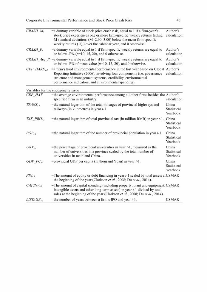
Corporate Environmental Performance and Stock Price Crash Risk 43

CRASH_Mt = a dummy variable of stock price crash risk, equal to 1 if a firm-year’s stock price experiences one or more firm-specific weekly returns falling M standard deviations (M=2.90, 3.00) below the mean firm-specific weekly returns (Wj,t) over the calendar year, and 0 otherwise.

Author’s calculation

CRASH_Pt = a dummy variable equal to 1 if firm-specific weekly returns are equal to or below -P% (p=10, 15, 20), and 0 otherwise.

Author’s calculation

CRASH_Avg_Pt = a dummy variable equal to 1 if firm-specific weekly returns are equal to or below -P% of mean value (p=10, 15, 20), and 0 otherwise.

Author’s calculation

CEP_HARDt-1 = a firm’s hard environmental performance in the last year based on Global Reporting Initiative (2006), involving four components (i.e. governance structure and management systems, credibility, environmental performance indicators, and environmental spending).

Author’s calculation

Variables for the endogeneity issue CEP_HAT = the average environmental performance among all other firms besides the

specified firm in an industry. Author’s calculation

TRANSt-1 = the natural logarithm of the total mileages of provincial highways and railways (in kilometres) in year t-1.

China Statistical Yearbook

TAX_PROt-1 = the natural logarithm of total provincial tax (in million RMB) in year t-1. China Statistical Yearbook

POPt-1 = the natural logarithm of the number of provincial population in year t-1. China Statistical Yearbook

UNVt-1 = the percentage of provincial universities in year t-1, measured as the number of universities in a province scaled by the total number of universities in mainland China.

China Statistical Yearbook

GDP_PCt-1 = provincial GDP per capita (in thousand Yuan) in year t-1. China Statistical Yearbook

FINt-1 = The amount of equity or debt financing in year t-1 scaled by total assets at the beginning of the year (Clarkson et al., 2008; Du et al., 2014).

CSMAR

CAPINVt-1 = The amount of capital spending (including property, plant and equipment, intangible assets and other long-term assets) in year t-1 divided by total sales at the beginning of the year (Clarkson et al., 2008; Du et al., 2014).

CSMAR

LISTAGEt-1 = the number of years between a firm’s IPO and year t-1. CSMAR