8/26/2019

1

Fall 2019

Prof. Ç. Çetinkaya

Chapter 2 Sections 2.1 – 2.2

Response to Harmonic Excitation

1

http://www.youtube.com/watch?v=UB9gA9Af5Tw&feature=related

Section 2.1 Harmonic Excitation of Undamped Systems

m k

x

F=Fo cost Consider the spring-mass damper

system with the following applied

(external) force:

ω is the driving frequency (important

note: this is not ωn)

F0 is the magnitude of the applied force

For simplicity, let us take c = 0 (no

damping case) to start with.

A Thought Experiment …

( ) cos( )oF t F t

2

Equations of Motion: c = 0

( ) cos( )px t X t

0

2

0

00

( ) ( ) cos( )

( ) ( ) cos( )

where ,

n

n

mx t k x t F t

x t x t f t

F kf

m m

The total Solution is the sum of homogenous solution ( xh(t) ) and

particular solution ( xp(t) ).

Propose the particular solution has the form of the forcing function:

F.B.D.

3

Total Solution = Homogeneous Solution + Particular Solution

Substitute Particular Solution into EoM:

2

2 2 2 2

0 0

0

2 2

cos cos cos

Solving this equation for yields the amplitude:

p n px x

n n

n

X t X t f t X X f

fX X

Thus, the particular solution has

the following form:

0

2 2( ) cos( )p

n

fx t t

4

( ) cos( )px t X t

Plug the particular soln (xp(t)) in the EoM to test if it works. And if it does,

determine its amplitude, X = ? :

2

0( ) ( ) cos( )nx t x t f t

8/26/2019

2

Total Solution Total Solution = Homogeneous Solution + Particular Solution

solution ( ( ))

01 2 2 2

homogeneous solution ( ( ))

( ) ( ) + ( )

( ) sin cos cos

p

h

h p

particular x t

n n

nx t

x t x t x t

fx t A t A t t

1 2 and are constants of integration. These constants for ( ) will be

determined from the I.C at = 0.

A A x t

t

Remark:

5

1 2

1 2

( ) sin( )

( ) sin cos

( ) n n

h n

h n n

j t j t

h

x t A t

x t A t A t

x t a e a e

Equivalent forms of homogenous solutions

n

k

m

0 0 01 2 2 0 2 02 2 2 2 2 2

(0) sin 0 cos0 cos0n n n

f f fx A A A x A x

Apply the I.C. to Determine A1 and A2

0 01 2 1 0 12 2

(0) cos0 sin 0 sin 0 n n n n

n n

f vx A A A v A

0 0 00 2 2 2 2

( ) sin cos cosn n

n n n

v f fx t t x t t

6

The general solution with the I.C. becomes:

1 2 2 2

homogeneous

( ) sin cos cos

particular

on n

n

fx t A t A t t

0

0

(0)

(0)

x x

x v

Comparison of Free and Forced Responses

Observations:

•Sum of two harmonic terms of different frequencies.

•Free response has amplitude and phase effected by forcing function (fo).

•Our solution is not defined for n = since it results in division by 0.

• If/when forcing frequency is close to natural frequency, the amplitude of

particular solution grows very large (singularity).

7

( )px t

Response for m = 100 kg, k = 1000 N/m, F = 100 N, = n + 5, v0=0.1m/s

and x0= -0.02 m.

Observe: The obvious presence of two harmonic signals

0 2 4 6 8 10 -0.05

0

0.05

Time (sec)

Dis

pla

ce

me

nt

(x)

Example: Time vs. Displacement Plot

8

0 0 00 2 2 2 2

( ) sin cos cosn n

n n n

v f fx t t x t t

1000 N/m3.16 rad/s 5 8.16 rad/s, 1

100 kgn n o

k Ff N kg

m m

8/26/2019

3

Example 2.1.1 Given for m = 10 kg, k = 1000 N/m, x0 = 0, v0 = 0.2 m/s, Fo = 23 N,

= 2 n.

Determine and plot the system’s response to this harmonic force

excitation.

9

m k

x

F=Fo cost

Example 2.1.1: Solution

00

0

2 2 2 2 2 2

1000 N/m10 rad/s 2 20 rad/s

10 kg

23 N 0.2 m/s2.3 N/kg 0.02 m

10 kg 10 rad/s

2.3 N/kg0.0076m

(10 20 ) rad / s

( ) 0.02sin10 0.0076(cos10 cos 20 )

n n

o

n

n

k

m

F vf

m

f

x t t t t

Compute and plot the response

m=10 kg, k=1000 N/m, x0=0, v0=0.2 m/s, Fo=23 N, =2n

10

0 0 00 2 2 2 2

( ) sin cos cosn n

n n n

v f fx t t x t t

Total solution:

Calculate parameters:

Plug these parameters into the total solution:

Example 2.1.1: Solution Compute and plot the response

( ) 0.02sin10 0.0076(cos10 cos 20 )x t t t t

11

time (sec)

x(t)

Example 2.1.2 Given zero initial conditions, a harmonic input of 10 Hz with 20 N magnitude

and k= 2000 N/m, and a measured response amplitude of 0.1 m, extract the

mass (m) of the system.

12

0

2 2cos cos n

n

ft t

0 0 00 2 2 2 2

( ) sin cos cosn n

n n n

v f fx t t x t t

Total Solution:

m k

x

F=Fo cost

8/26/2019

4

Example 2.1.2: Solution

0

2 2

0

2 2

0

2 2

0.1 m

0

2 22

( ) cos cos

cos 20 cos

2( ) sin sin

2 2

202

20.1 0.1 0.405 kg

2000(2 10)

n

n

n

n

n n

n

n

fx t t t

ft t

fx t t t

f m m

m

I.C.: at rest at t = 0

f =10 Hz with Fo=20 N

k= 2000 N/m

A max= 0.1m

m=? kg

13

This is not amplitude of x(t)

0oF

fm

Amplitude of x(t)

When the drive frequency

and natural frequency are

the same ( =n), the

amplitude of the vibration

grows with no bounds.

This is known as a

resonance condition.

( ) sin( )px t t X t

0 5 10 15 20 25 30 -5

0

5

Time (sec)

Dis

pla

ce

me

nt (x

)

grows without bound

01 2( ) sin cos sin( )

2

fx t A t A t t t

14

Form of the particular solution is:

The total solution becomes:

When =n, What is the Response?

0Substituting this into the EoM and solving for yields: 2

fX X

What Occurs When is Near n?

0

2 2

0

2 2

( ) cos cos

2sin sin

2 2

n

n

n n

n

fx t t t

ft t

Consider the simplified case, namely x(0) = v(0) = 0 (from rest)

0 0 00 2 2 2 2

( ) sin cos cosn n

n n n

v f fx t t x t t

15

General Solution:

Apply the zero initial conditions to obtain: Using the trig identify (sum-to-

product)

http://www.youtube.com/watch?v=5hxQDAmdNWE

0 5 10 15 20 25 30 -1

-0.5

0

0.5

1

Time (sec)

Dis

pla

ce

me

nt

(x)

sin when is small. Namely, the period is large. 2

nnt T

16

0

2 2

2( ) sin sin

2 2

n n

n

fx t t t

1T

What Occurs When is Near n?

8/26/2019

5

0 5 10 15 20 25 30 -1

-0.5

0

0.5

1

Time (sec)

Dis

pla

ce

me

nt

(x)

0

2 2

2( ) sin sin

2 2

n n

n

fx t t t

17

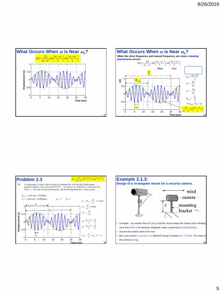
What Occurs When is Near n?

1T

When the drive frequency and natural frequency are close a beating

phenomena occurs.

0 5 10 15 20 25 30 -1

-0.5

0

0.5

1

Time (sec)

x(t

)

2 f0

n

2 2sin

n

2t

0

2 2

2( ) sin sin

2 2

n n

n

fx t t t

18

1

2

1

1

2

2

1

2

2

2

2

2

=

n

n

beat

beat n

T

T

TT

2T

beatT

What Occurs When is Near n?

Slow Fast

0 5 10 15 20 25 30 -1

-0.5

0

0.5

1

Time (sec)

Dis

pla

ce

me

nt

(x)

19

1T

2T

2

0.2 sec 0.628sec

0.02 sec 0.0628sec ? ?

beat

n

T

T

Problem 2.3

beatT

0

2 2

2( ) sin sin

2 2

n n

n

fx t t t

1

1

2

2

1

1

2

2

1

2 2 2 0.628

2 0.0628

2

2 =

2

2 =

2

=2

beat

beat

beat

n

n

beat beat n

T T

T

T

T

T

TT

Example 2.1.3:

• Compute l (no shorter than 0.5 m) so that the mount keeps the camera from vibrating

more then 0.01 m of maximum amplitude under a wind load of 15 N at 10 Hz.

• Assume the motion starts from rest.

• Bar cross section: 2 cm by 2 cm. Material Young’s modulus: E = 71 GPa. The mass of

the camera is 3 kg.

Design of a rectangular mount for a security camera.

20

8/26/2019

6

Example 2.1.3: Solution/Modeling

21

Example 2.1.3: Solution

03

3( ) cos

EIm x x t F t

From the strength of materials (beam bending):

3

12

bhI

Thus, the frequency expression becomes:

3 32

3 3

3

12 4n

E b h E b h

m m

Modeling the mount and camera as a beam with a tip mass,

and the wind as harmonic, the equation of motion becomes:

22

l = ?, lmin = 0.5 m

A max = 0.01 m

Fo = 15 N

f = 10 Hz

m = 3 kg

Cross-section: 2 by 2 cm

E = 71 GPa

2

3

3since and n

EI kk

l m

23

0

2 2

0

2 2

( ) cos cos

2sin sin

2 2

n

n

n n

n

fx t t t

ft t

0 0 00 2 2 2 2

( ) sin cos cosn n

n n n

v f fx t t x t t

Example 2.1.3: Solution Total Solution:

Task: Compute l, making the amplitude less than 1 cm

0 0

2 2 2 2

2 20.01 0.01 0.01

n n

f f

32

34n

E b h

m

Amplitude of x(t)

Case A:

0 0 0

2 2 2 2 2 2

32 2 2

0 0 3

33

2

0

2 2 20.01 0.01

0.01( ) 2 0.01 2 0.014

0.01 0.321 0.685 m4 (0.01 2 )

n n n

n

f f f

Ebhf f

m

Ebh

m f

Example 2.1.3: Solution

24

2 2For 0 namely, n n

Here we are interested computing l that will make the amplitude less

than 0.01 m =1 cm: 2 20

2 2

0 0

2 2 2 22 20

2 2

2Case A 0.01 0, for 0

2 20.01 0.01 0.01

2Case B 0 < 0.01, for 0

n

n

n nn

n

f

f f

f

l = ?, lmin = 0.5 m

A max = 0.01 m

Fo = 15 N

f = 10 Hz = 2π f

m = 3 kg

Cross-section: 2 by 2 cm

E = 71 GPa

32

34n

E bh

m

8/26/2019

7

Case B:

32 2 20

0 02 2 3

33

2

0

20.01 2 0.01( ) 2 0.01 0.01

4

0.01 0.191 0.576 m4 (2 0.01 )

n

n

f Ebhf f

m

Ebh

m f

Example 2.1.3: Solution

25

2 2For 0 namely, n n

l = ?, lmin = 0.5 m

A max = 0.01 m

Fo = 15 N

f = 10 Hz = 2π f

m = 3 kg

Cross-section: 2 by 2 cm

E = 71 GPa

32

34n

E bh

m

Constraint: The length must be at least 0.5 m, (A) and (B) yield:

> 0.685 m (Case A) or 0.5 0.576 (Case B)

Case A:

0

2 2

20.01 0.685 m

n

f

Constraint: the length must be at least 0.5 m, (A) and (B) yield:

> 0.685 m (Case A) or 0.5 0.576 (Case B)

It is desirable that the resonance freq is higher than the excitation freq (also less material is usually desirable), so choose Case B, say l = 0.55 m. To

check the resonance frequency is higher than the excitation frequency, note that for l = 0.55:

3

22 2

3

320 1742 0

12n

Ebh

m

Thus, Case B condition is satisfied. Next check the mass of the designed beam

if low. This is to make certain that it does not affect the frequency:

Observation: It is much less then the camera mass m = 3kg, thus it is (border

line) negligible.

2700 0.55 0.02 0.02 0.59 kgbeamm b h

Example 2.1.3: Design Considerations

26

2

0 0( ) ( ) sin or ( ) ( ) sin nm x t k x t F t x t x t f t

The particular solution then becomes a sine: ( ) sin px t X t

Substitution of this solution into the EoM

above yields, the particular solution:

0

2 2( ) sinp

n

fx t t

Solving for the homogenous solution and evaluating the constants

yields the total solution for this type of excitation as:

0 0 00 2 2 2 2

( ) cos sin sin n n

n n n n

v f fx t x t t t

External Excitation: F(t) = sin( t)

27

Section 2.2 Harmonic Excitation of Damped Systems

28

• Harmonically excited systems with damping, c ≠ 0

• Extending resonance and response calculation to damped

systems

8/26/2019

8

Harmonic Excitation of Damped Systems

2

0 0( ) ( ) ( ) cos ( ) 2 ( ) ( ) cosn nm x t c x t k x t F t x t x t x t f t

m

k x

c

29

Steady State (Particular) Transient (Homogeneous) Solution, ( ) Solution, ( )

( ) sin( ) cos( )n

ph

t

d

x tx t

x t Ae t X t

2

2

1 d n

n

o

c=

km

k

m

Ff

m

0 cosF F t

Free Body Diagram:

( )F tSteady state (particular) solution

2 2 1

( ) cos( ) cos sin

tan

p s s

ss s

s

x t X t A t B t

BX A B

A

Assume that the particular solution xp(t) has the following form:

Note: The rectangular form/representation is used here, but we could use

one of the other forms/representations of the solution.

Determining the Integration Constants

2 2

sin cos

cos sin

p s s

p s s

x A t B t

x A t B t

30

1 2

1 2

( ) sin( )

( ) sin cos

( ) n n

n

n n

j t j t

x t A t

x t A t A t

x t a e a e

2

0( ) 2 ( ) ( ) cosn nx t x t x t f t

As = ? Bs=?

2 2

0

2 2

( ) (2 ) 0

( 2 ) ( ) 0

n s n s

n s n s

A B f

A B

Substitute these into the EoM to obtain, a characteristic equation:

2 2

0

2 2

( 2 )cos

2 sin 0

s n s n s

s n s n s

A B A f t

B A B t

31

This equation is satisfied for all t if and only if both coefficients satisfy the

following conditions simultaneously:

Determining the Integration Constants

Express these two equations as a matrix equation:

2 20

2 2

12 2

0

2 2

( ) 2

02 ( )

( ) 2

02 ( )

sn n

sn n

s n n

s n n

A f

B

A f

B

2 2

0

2 2 2 2

0

2 2 2 2

( )

( ) (2 )

2

( ) (2 )

ns

n n

ns

n n

fA

fB

Solving for As and Bs yields:

32

Inverse:

Matrix:

Determining the Integration Constants

8/26/2019

9

10

2 22 2 2 2

2( ) cos tan

( ) (2 )

np

nn n

X

fx t t

Substitute the values of As and Bs into the particular solution xp:

Total Solution = Homogeneous Solution + Particular Solution

Remarks:

A and are determined from the I.C. in the total solution. In general, these do

not have the same values as in the free response.

As t tends to infinitely, transient dies out to the exponential term.

Total Solution

33

1 2

1 2

( ) sin( )

( ) sin cos

( ) n n

n

n n

j t j t

x t A t

x t A t A t

x t a e a e

Steady State (Particular) Transient (Homogeneous)

Solution, ( ) Solution, ( )

( ) sin( ) cos( )n

ph

t

d

x tx t

x t Ae t X t

34

1 2

1 2

( ) sin( )

( ) sin cos

( ) n n

n

n n

j t j t

x t A t

x t A t A t

x t a e a e

Response of Under-damped Systems

Steady State (Particular) Transient (Homogeneous) Solution, ( ) Solution, ( )

( ) sin( ) cos( )n

ph

t

d

x tx t

x t Ae t X t

Remarks: Damped Forced Response

• If = 0, un-damped equations result in

• Steady state solution prevails for large t (long time-scale)

• Often we ignore the transient term (how large is , how long is t?)

• Coefficients of transient terms (constants of integration) are affected by the initial conditions and the forcing function

• For under-damped systems at resonance, the amplitude is finite.

35

As (n

2 2 ) f0

(n

2 2 )2 (2n )2

Bs 2n f0

(n

2 2 )2 (2n )2

Steady-State (Particular) Solution

( ) cos( ) cos sinp s sx t X t A t B t

Steady-State (Particular) Transient (Homogeneous) Solution, ( ) Solution, ( )

( ) sin( ) cos( )n

ph

t

d

x tx t

x t Ae t X t

Example 2.2.1:

Given that n = 10 rad/s, = 5 rad/s, = 0.01, F0= 1000 N,

m = 100 kg, and the initial conditions x0 = 0.05 m and v0 = 0.

No damping, c=0.

Compute the integration constants.

Compare these to no external forcing case.

36

Important Note:

Solution to this problem in the textbook (3rd Edition) is incorrect.

0 cosF F t

m

k x

c

8/26/2019

10

Example 2.2.1: Solution

2

0.1

0.133 0.013 0.1

1 9.99 / sec

( ) sin(9.99 ) 0.133cos(5 0.013)

n

d n

t

X m rad

rad

x t Ae t t

Using these equations:

n = 10 rad/s, = 5 rad/s, = 0.01, F0= 1000 N, m = 100 kg

I.C. x0 = 0.05 m and v0 = 0. No damping: c=0.

10

2 22 2 2 2

2( ) cos( tan )

( ) (2 )

np

nn n

X

fx t t

( ) sin( )nt

h dx t Ae t

37

Example 2.2.1: Solution

0.1 0.1( ) 0.1 sin(9.99 ) 9.99 cos(9.99 ) 0.665sin(5 0.013)t tx t Ae t Ae t t

Differentiating x(t) yields:

(0) 0.05 sin 0.133cos( 0.013)

(0) 0 0.01 sin 9.999 cos 0.665sin 0.013

x A

v A A

0.1( ) sin(9.99 ) 0.133cos(5 0.013)tx t Ae t t

Applying the ICs, (0) = 0.05m, (0) 0 and solving these two equations

for and results in:

0.519

0.875

x x

A

A m

rad

38

?

?

A

39

Problem 2.30: Solution Hints

2

0.05

oI m l

a m

sF cF

θ

0

2

0

( ) ( ) ( ) cos

( ) 2 ( ) ( ) cosn n

m x t c x t k x t F t

x t x t x t f t

x ↔ θ

O o

On Ignoring the Transient Response

• Always check to make sure the transient (particular solution) is

insignificant for the problem/application at hand;

• Compare transient amplitude to that of homogenous solution;

• For example, transients are very important in earthquakes;

• In many machine design applications, transients may be ignored.

40

8/26/2019

11

Static Displacement

41

0F

m

k

x

c

0

00

FF k x x

k

0

Magnitude:

Non dimensional

form of disp.:

Frequency ratio:

0

2 2 2 2 2 2 2 20

1

( ) (2 ) ( ) (2 )n n n n

f XX

f

2

2 2 2 20 0 02

2 2 2 2 2 2 2

2 2

1

1( ) (2 )

1 1

( ) (2 ) (1 ) (2 )

n

n n

n

n n

n n

dynamic X X k X

static F k m f f

r r

n

n

kr

m

Steady-State Solution (Response): t → ∞

42

12

2 tan

12

c rrk m

Damping ratio:

Steady-State (Particular) Transient (Homogeneous) Solution, ( ) Solution, ( )

( ) sin( ) cos( )n

ph

t

d

x tx t

x t Ae t X t

00

0

F

F k x xk

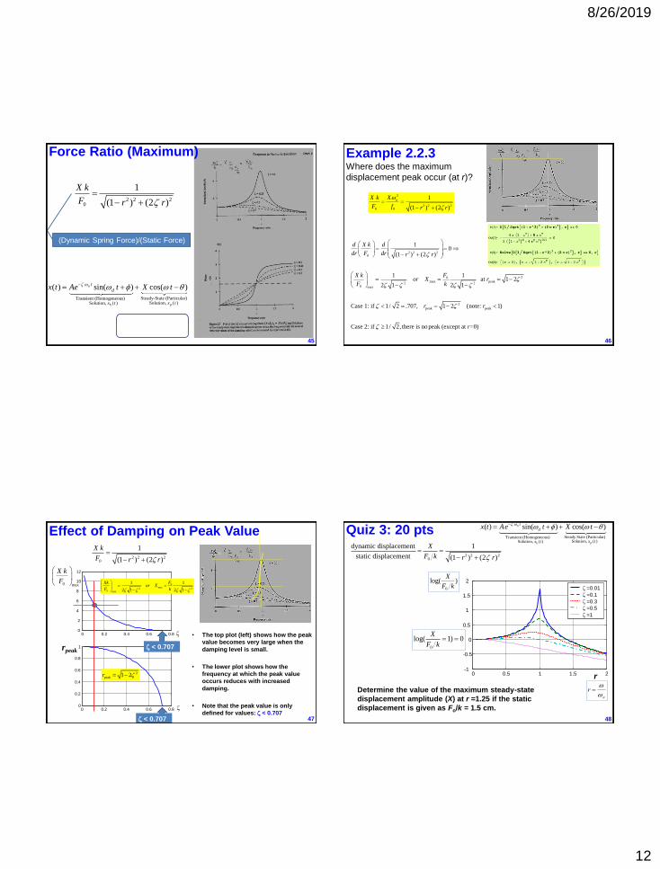
Magnitude Plot: Steady-State Response

0 0.5 1 1.5 2 -1

-.05

0

0.5

1

1.5

2

r

=0.01

=0.1

=0.3

=0.5

=1

• Resonance is close to r = 1

• For = 0, r =1 defines

resonance

• As grows resonance

moves r <1, and X decreases

• The exact value of r can be

found from maximizing the

magnitude.

43

r

n

2 2 20

dynamic displacement 1

static displacement (1 ) (2 )

X

F k r r

0

log( )X

F k

Steady State (Particular) Transient (Homogeneous) Solution, ( ) Solution, ( )

( ) sin( ) cos( )n

ph

t

d

x tx t

x t Ae t X t

log(1) 0

0

log( 1) 0X

F k

• Resonance occurs at = /2

• The phase changes more rapidly

when the damping is small

• From low to high values of r the

phase always changes by 1800 or

radians

0 0.5 1 1.5 2 0

0.5

1

1.5

2

2.5

3

3.5

r

Ph

as

e (ra

d)

=0.01

=0.1

=0.3

=0.5

=1

12

2tan1

rr

Phase Plot: Steady State Response

44

/2

r

n

Steady State (Particular) Transient (Homogeneous) Solution, ( ) Solution, ( )

( ) sin( ) cos( )n

ph

t

d

x tx t

x t Ae t X t

8/26/2019

12

45

12

2tan

1r

r

2 2 20

1

(1 ) (2 )

X k

F r r

(Dynamic Spring Force)/(Static Force)

Force Ratio (Maximum)

Steady-State (Particular) Transient (Homogeneous) Solution, ( ) Solution, ( )

( ) sin( ) cos( )n

ph

t

d

x tx t

x t Ae t X t

2 2 20

20max peak

2 20 max

2

peak peak

10

(1 ) (2 )

1 1 at 1 2

2 1 2 1

Case 1: if 1 / 2 .707, 1 2 (note: 1)

Case 2: if 1 / 2, there is no peak (except at =0)

d X k d

dr F dr r r

X k For X r

F k

r r

r

Example 2.2.3 Where does the maximum

displacement peak occur (at r)?

46

2

2 2 20 0

1

(1 ) (2 )

nX k X

F f r r

Effect of Damping on Peak Value

0 0.2 0.4 0.6 0.8 0

2

4

6

8

10

12

0 0.2 0.4 0.6 0.8 0

0.2

0.4

0.6

0.8

1

rpeak

0 max

X k

F

• The top plot (left) shows how the peak

value becomes very large when the

damping level is small.

• The lower plot shows how the

frequency at which the peak value

occurs reduces with increased

damping.

• Note that the peak value is only

defined for values: < 0.707 47

2 2 20

1

(1 ) (2 )

X k

F r r

< 0.707

< 0.707

0max

2 20 max

1 1

2 1 2 1

FXkor X

F k

2

peak 1 2r

Quiz 3: 20 pts

0 0.5 1 1.5 2 -1

-0.5

0

0.5

1

1.5

2

r

=0.01

=0.1

=0.3

=0.5

=1

Determine the value of the maximum steady-state

displacement amplitude (X) at r =1.25 if the static

displacement is given as Fo/k = 1.5 cm.

48

r

n

2 2 20

dynamic displacement 1

static displacement (1 ) (2 )

X

F k r r

0

log( )X

F k

Steady State (Particular) Transient (Homogeneous) Solution, ( ) Solution, ( )

( ) sin( ) cos( )n

ph

t

d

x tx t

x t Ae t X t

0

log( 1) 0X

F k