1

Clustering via Kernel DecompositionA. Szymkowiak-Have∗, M.A.Girolami †, Jan Larsen∗

∗Informatics and Mathematical ModellingTechnical University of Denmark, Building 321

DK-2800 Lyngby, DenmarkPhone: +45 4525 3899,3923

Fax: +45 4587 2599E-mail: asz,jl@imm.dtu.dk

Web: isp.imm.dtu.dk†School of ICT, University of Paisley

High Street, Paisley, UKPhone: +44 141 848 3317

Fax: +44 141 848 3542E-mail: mark.girolami@paisley.ac.uk

Abstract— Spectral clustering methods were proposed recentlywhich rely on the eigenvalue decomposition of an affinity matrix.In this work the affinity matrix is created from the elements of anon-parametric density estimator and then decomposed to obtainposterior probabilities of class membership. Hyperparametersare selected using standard cross-validation methods.

Index Terms— spectral clustering, kernel decomposition, ag-gregated Markov model, kernel principal component analysis

I. INTRODUCTION

The spectral clustering methods [1], [2], [3] are attractivein the case of complex data sets, which possess for examplemanifold structures, when the classical models such as K-means often fail in the correct estimation. The proposedmodels in the literature are, however, incomplete, since theydo not offer methods for the estimation of the model hyper-parameters which have to be manually tuned [1]. The needarises to construct a self-contained model, which would notonly provide accurate clustering but also which would estimateboth the model complexity and all the necessary parametersfor estimation. The additional advantage can also be providedby the probabilistic outcome, where the confidence in the pointassignment to the clusters is given.

The kernel principal component analysis (KPCA) [4] de-composition of a Gram matrix has been shown to be aparticularly elegant method for extracting nonlinear featuresfrom multivariate data. KPCA has been shown to be a dis-crete analogue of the Nystrom approximation to obtainingthe eigenfunctions of a process from a finite sample [5].Building on this observation the relationship between KPCAand non-parametric orthogonal series density estimation washighlighted in [6], and the relation with spectral clustering hasrecently been investigated in [7]. The basis functions obtainedfrom KPCA can be viewed as the finite sample estimates of thetruncated orthogonal series [6], however, a problem commonto orthogonal series density estimation is that the strict non-negativity required of a probability density is not guaranteed

when employing these finite order sequences to make pointestimates [8], this is of course also observed with the KPCAdecomposition [6].

To further explore the relationship between the decompo-sition of a Gram matrix, the basis functions obtained fromKPCA and density estimation, a matrix decomposition whichmaintains the positivity of point probability density estimatesis desirable. In this paper we show that such a decompositioncan be obtained in a straightforward manner and we observeuseful similarities between such a decomposition and spectralclustering methods [1], [2], [3].

The following sections consider the non-parametric estima-tion of a probability density from a finite sample [8] and relatesthis to the identification of class structure within the densityfrom the sample. Two kernel functions, the choice of whichdependent on the data type and dimensionality, are proposed.The derivation of the generalization error is also presented,which enables the determination of the model parameters andmodel complexity [9], [10]. The experiments are performedon artificial data sets as well as on more realistic collections.

II. DENSITY ESTIMATION AND DECOMPOSITION OF THEGRAM MATRIX

Consider the estimation of an unknown probability densityfunction p(x) from a finite sample of N points {x1, · · · ,xN}where x ∈ Rd. The sample drawn from the density can beemployed to estimate the density in a non-parametric form byusing a Parzen window estimator (refer to [8], [9], [10] fora review of such non-parametric density estimation methods)such that the estimate is given by

p(x) =1

N

N∑

n=1

Kh(x,xn) (1)

where Kh(xi,xj) denotes the kernel function of width h,between points xi and xj , which itself satisfies the require-ments of a density function [8]. It is important to note that

the pairwise kernel function values Kh(xi,xj) provide thenecessary information regarding the sample estimate of theunderlying probability density function p(x). Therefore thekernel or Gram matrix constructed from a sample of points(and a kernel function which itself is a density) provides thenecessary information to faithfully reconstruct the estimateddensity from the pairwise kernel interactions in the sample.

For applications of unsupervised kernel methods such asKPCA the selection of the kernel parameter, in the case of theGaussian kernel h, is often problematic. However, noting thatthat the kernel matrix can be viewed as defining the sampledensity estimate, then methods such as leave-one-out cross-validation can be employed in obtaining an appropriate valueof the kernel width parameter. We shall return to this point inthe following sections.

A. Kernel Decomposition

The density estimate can be decomposed in the followingprobabilistic manner as

p(x) =

N∑

n=1

p(x,xn) (2)

=

N∑

n=1

p(x|xn)P (xn) (3)

such that each sample point is equally probable a priori,P (xn) = N−1, i.e. data is assumed independent and iden-tically distributed (i.i.d). The kernel operation, such that thekernel is itself a density function, can then be seen to be theabove conditional density p(x|xn) = Kh(x,xn).

The sample of N points drawn from the underlying densityforms a set and as such we can define a probability space overthe N points. A discrete posterior probability can be definedfor a point x (either in or out of sample) given each of the N

sample points

P (xn|x) =p(x|xn)P (xn)

∑N

n′=1p(x|xn′)P (xn′)

=K(x,xn)

∑N

n′=1K(x,xn′)

≡ K(x,xn) (4)

such that∑N

n=1P (xn|x) = 1, P (xn|x) ≥ 0 ∀ n and each

P (xn) = 1

N.

Now if it is assumed that there is an underlying, hiddenclass/cluster structure in the density then the sample posteriorprobability can be decomposed by introducing a discrete classvariable such that

P (xn|x) =

C∑

c=1

P (xn, c|x) =

C∑

c=1

P (xn|c,x)P (c|x) (5)

and noting that the sample points have been drawn i.i.d fromthe respective C classes forming the distribution such thatxn⊥x | c, then

P (xn|x) =C

∑

c=1

P (xn, c|x) =C

∑

c=1

P (xn|c)P (c|x) (6)

with constraints∑N

n=1P (xn|c) = 1 and

∑C

c=1P (c|x) = 1.

Considering the decomposition of the posterior sampleprobabilities for each point in the available sample P (xi|xj) =∑C

c=1P (xi|c)P (c|xj), ∀ i, j = 1, · · · , N we see that this is

identical to the aggregate Markov model originally proposedby Saul and Periera [11], where the matrix of posteriors(elements of the normalized kernel matrix) can be now beviewed as an estimated state transition matrix for a firstorder Markov process. This decomposition then provides classposterior probabilities P (c|xn) which can be employed forclustering purposes.

A divergence based criterion such as cross-entropyN

∑

i=1

N∑

j=1

K(xi,xj) log

{

C∑

c=1

P (xi|c)P (c|xj)

}

(7)

or distance based criterion such as squared error

N∑

i=1

N∑

j=1

{

K(xi,xj) −

{

C∑

c=1

P (xi|c)P (c|xj)

}}2

(8)

can be locally optimized by employing the standard non-negative matrix multiplicative update equations (NMF) [12],[13] or equivalently the iterative algorithm which performsProbabilistic Latent Semantic Analysis (PLSA) [14]. If thenormalized Gram matrix is defined as G = {P (xi,xj)} =K(xi,xj) then the decomposition of that matrix with NMF[12], [13] or PLSA [14] algorithms will yield G = WH suchthat W = {P (xi|c)} and H = {P (c|xj)} are understood asthe required probabilities which satisfy the previously definedstochastic constraints.

B. Clustering with the Kernel Decomposition

Having obtained the elements P (xi|c) and P (c|xj) of thedecomposed matrix employing NMF or PLSA, the class poste-riors P (c|xj) will indicate the class structure of the samples.We are now in a position to assign newly observed out-of-sample points to a particular class. If we observe a new pointz in addition to the sample then the estimated decompositioncomponents can, in conjunction with the kernel, provide therequired class posterior P (c|z).

P (c|z) =

N∑

n=1

P (c|xn)P (xn|z) (9)

=

N∑

n=1

P (c|xn)K(z,xn) (10)

=N

∑

n=1

P (c|xn)K(z,xn)

∑N

n′=1K(z,xn′)

(11)

This can be viewed as a form of ’kernel’ based non-negativematrix factorization where the ’basis’ functions P (c|xn) definethe class structure of the estimated density.

For the case of a Gaussian (radial basis function) kernelthis interpretation of a kernel based clustering motivates thedefinition of the kernel smoothing parameter by means of out-of sample predictive likelihood and as such cross-validationcan be employed in estimating the kernel width parameter.In addition the problem of choosing the number of possible

2

classes, a problem common to all non-parametric clusteringmethods such as spectral clustering [1],[15] can now beaddressed using theoretically sound model selection methodssuch as cross-validation. This overcomes the lack of an objec-tive means of selecting the smoothing parameter in most otherforms of spectral clustering [1],[15] as the proposed methodfirst defines a non-parametric density estimate, and then theinherent class structure is identified by the basis decompositionof the normalized kernel in the form of class conditionalposterior probabilities. This highlights another advantage, overpartitioning based methods [1], [15], of this view on kernelbased clustering in that projection coefficients are providedenabling new or previously unobserved points to be allocatedto clusters. Thus projection of the normalized kernel functionof a new point onto the class-conditional basis functions willyield the posterior probability of class membership for the newpoint.

In attempting to identify the model order, eg. number ofclasses, a generalization error based on the out-of-samplenegative predictive likelihood, is defined as follow

Lout = N−1

out

Nout∑

n=1

log {p(zn)} (12)

where Nout denotes the number of out-of-sample points. Theout-of-sample likelihood (12) is derived from the decomposi-tion in the following manner

p(z) =1

N

N∑

n=1

p(z|xn) (13)

=1

N

N∑

n=1

C∑

c=1

p(z|c)P (c|xn) (14)

The p(z|c) can be decomposed given the finite sample suchthat p(z|c) =

∑N

l=1p(z|xl)P (xl|c) where p(z|xl) = K(z|xl).

So the unconditional density estimate of an out of samplepoint given the current kernel decomposition which assumesa specific class structure in the data can be computed as thefollowing.

p(z) =1

N

N∑

n=1

N∑

l=1

C∑

c=1

K(z|xl)P (xl|c)P (c|xn), (15)

where P (xl|c) = W and P (c|xn) = H are estimatedparameters.

C. Kernels

For continuous data such that x ∈ Rd a common choiceof kernel, for both kernel PCA and density estimation, is theisotropic Gaussian kernel

Kh(x,xn) = (2π)−d

2 h−d exp

{

−1

2h2||x − xn||

2

}

(16)

Of course many other forms of kernel can be employed,though they may not themselves satisfy the requirements ofbeing a density. In the case of discrete data such as vector

space representations of text we consider for example thelinear cosine inner-product

K(x,xn) =x

Txn

||x|| · ||xn||. (17)

The decomposition of this cosine based Gram matrix directlywill yield the required probabilities.

Although, the cosine inner-product does not satisfy itselfthe density requirements (

∫

K(x,xn) = 1) it can be appliedin the presented model as long as the kernel integral is finite.This condition is satisfied when the data points are a priorinormalized, e.g. to the unit sphere and the empty vectors areexcluded from the data set. The density values obtained fromsuch non-density kernels provide the incorrect generalizationerrors which are scaled by the unknown constant factor andtherefore can be still used in estimation of the parameters.

This interpretation provides a means of spectral clusteringwhich, in the case of continuous data, is linked directly to non-parametric density estimation and extends easily to discretedata such as for example text. We should also note that theaggregate Markov perspective allows us to take the randomwalk viewpoint as elaborated in [15] and so a K-connectedgraph1 may be employed in defining the kernel similarityKK(x,xn). Similarly to the smoothing parameter and thenumber of clusters, the number of connected points in thegraph can be also estimated from the generalization error.

The following experiments and subsequent analysis providean objective assessment and comparison of a number ofclassical and recently proposed clustering methods.

III. EXPERIMENTS

In the experiments we used, the four following data setsdescribed below.

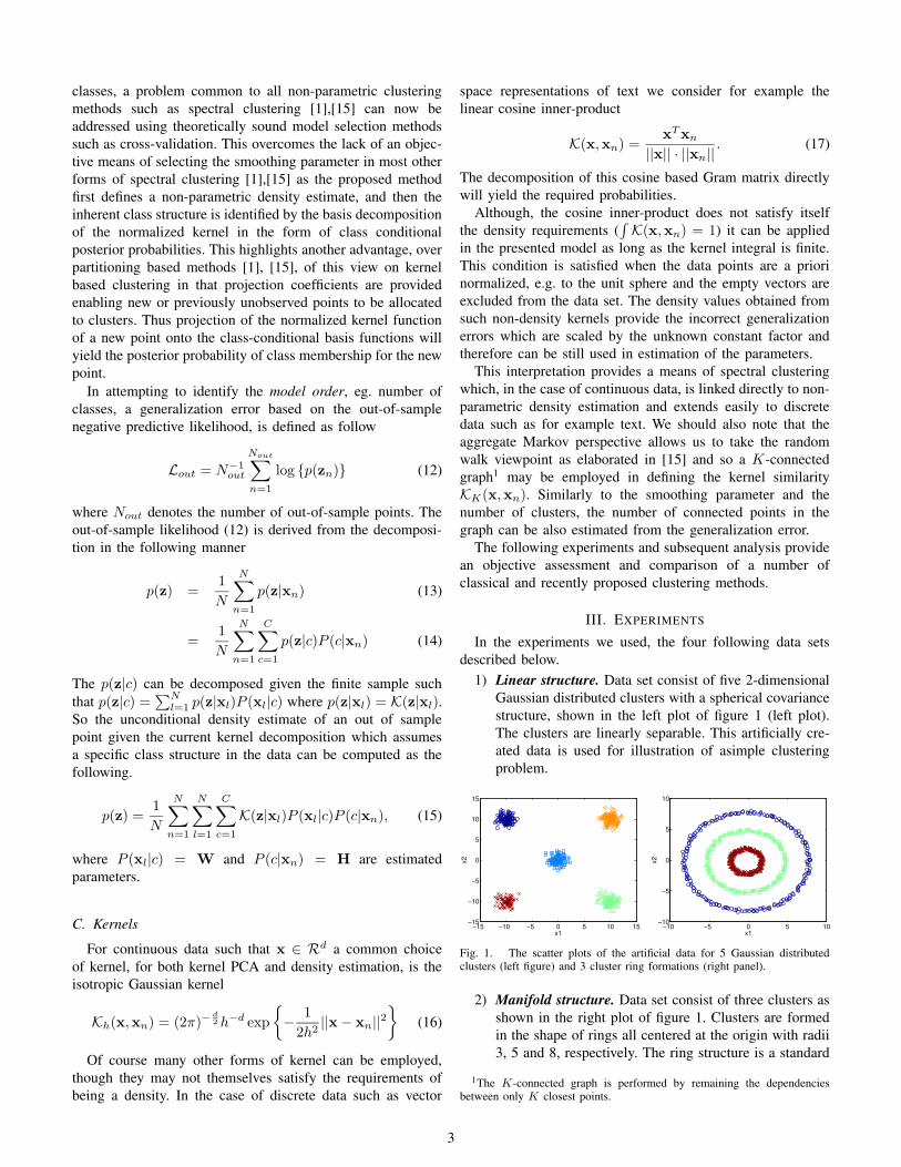
1) Linear structure. Data set consist of five 2-dimensionalGaussian distributed clusters with a spherical covariancestructure, shown in the left plot of figure 1 (left plot).The clusters are linearly separable. This artificially cre-ated data is used for illustration of asimple clusteringproblem.

−15 −10 −5 0 5 10 15−15

−10

−5

0

5

10

15

x1

x2

−10 −5 0 5 10−10

−5

0

5

10

x1

x2

Fig. 1. The scatter plots of the artificial data for 5 Gaussian distributedclusters (left figure) and 3 cluster ring formations (right panel).

2) Manifold structure. Data set consist of three clusters asshown in the right plot of figure 1. Clusters are formedin the shape of rings all centered at the origin with radii3, 5 and 8, respectively. The ring structure is a standard

1The K-connected graph is performed by remaining the dependenciesbetween only K closest points.

3

example used in spectral clustering, for example [1], [2].The data is 2 dimensional. This is given as an exampleof complex nonlinear data on which methods such asK-means will fail.

3) Email collection. The Email data set2 consist of emailsgrouped into three categories: conference, job and spam,used earlier in [16], [17], [18]. The collection was hand-labeled. In order to process text data a term-vector isdefined as the complete set of all the words existingin all the email documents. Then each email documentis represented by a histogram: the frequency vector ofoccurrences of each of the word from a term-vector. Thecollection of such email histograms is denoted the term-document matrix. In order to achieve good performance,suitable preprocessing is performed. It includes remov-ing stopwords3 and other high and low frequency words,stemming4 and normalizing histograms to unit L2-normlength. After preprocessing, the term-document matrixconsist of 1405 email histograms described by 7798terms. The data points are discrete and high dimensionaland the categories are not linearly separable.

4) Newsgroups. The collection5 consist originally of 20categories each containing approximately 1000 news-group documents. In the performed experiments 4 cat-egories (computer graphics, motorcycles, baseball andChristian religion) were selected each containing 200instances. The labels of the collection are selected basedon the catalogs names the data was stored in. Thedata was processed in a similar way as that presentedabove. In preprocessing 2 documents were removed6.After preprocessing the data consists of 798 newsgroupdocuments described in the space of 1368 terms.

In the case of continuous space collections (Gaussian andRings clusters) data vectors were normalized with its maxi-mum value so, they fall in the range between 0 and 1. Thisstep is necessary when the features describing data points havesignificantly different values and ranges. The normalizationto the unit L2-norm length was applied for the Email andNewsgroup collections.

For Gaussian and Rings clusters the isotropic Gaussiankernel equation (16) is used. With discrete data sets (Emailsand Newsgroups) the cosine inner-product equation (17) isapplied.

The Gaussian clusters example is a simple linear separa-tion problem. The model was trained using 500 randomlygenerated samples, and generalization error computed from2500 validation set samples. The aggregated Markov model,as a probabilistic framework, allows the new data points, notincluded in the training set, to be uniquely mapped in the

2The Email database ia available at http://isp.imm.dtu.dk/staff/anna3Stopword are high frequency words that are helping to build the sentence,

e.g. conjunctions, pronouns, prepositions etc. A list of 584 stopwords is usedin the experiments

4Stemming denotes the process of merging words with typical endings intothe common stem. For example for English language the endings like e.g.-ed, -ing, -s are considered.

5The Newsgroups collection is available at e.g. http://kdd.ics.uci.edu/6Reduction in term space (stopwords removing, stemming, etc. ) resulted

with empty documents, which were removed from the data set.

0 0.1 0.2 0.3 0.4 0.502468

101214161820

h − smoothing parameter

Gen

eral

izat

ion

erro

r

5 Gaussian clusters

0.04 0.06 0.08 0.1−0.4

−0.3

−0.2

−0.1

0

h

Gen

. err

or

2 3 4 5 6 7 8 9 10−326

−324

−322

−320

−318

−316

x 10 −3

c − number of clusters

Gen

eral

izat

ion

erro

r

5 Gaussian clusters

−0.3

2516

86

−0.3

2516

78

−0.3

2516

86

−0.3

2516

87

Fig. 2. The generalization error as a function of smoothing parameter h (leftpanel) for 5 Gaussian distributed clusters. The optimum choice is h = 0.06.The right figure presents, for optimum smoothing parameter, the generalizationerror as a function of number of clusters. Here, any cluster number below orequal 5 may give the minimum error for which the error values are shownabove the points. The optimum choice is a maximum model, i.e. K = 5 (seethe explanation in the text). The error-bars show ± standard error of the meanvalue.

model. It is possible to select optimum model parameters: h,K in K-connected graph in discrete data sets and the optimumnumber of clusters c by minimizing the generalization errordefined by the equations (12) and (14).

In 20 experiments, different training sets were generated,and the final error is an average over 20 outcomes of thealgorithm on the same validation set. The left plot of figure2 presents the dependency of the generalization error as afunction of the kernel smoothing parameter h, averaged forall the model orders. The minimum is obtained for h = 0.06.For that optimum h the model complexity c is then investigated(right plot of figure 2). Here, the minimal error is obtained forall 2, 3, 4 and 5 clusters and as the optimal solution 5 clustersare chosen, which is explained in appendix .

For Gaussian clusters the cluster posterior p(c|z) is pre-sented on figure 3. Perfect decision surfaces can be observed.For comparison, on figure 4, the components of the traditional

−1 −0.5 0 0.5 1−1

−0.50

0.51

0

0.5

1

CLUSTER 1

p(c=

1|z)

−1 −0.5 0 0.5 1−1

−0.50

0.51

0

0.5

1

CLUSTER 2

p(c=

2|z)

−1 −0.5 0 0.5 1−1

−0.50

0.51

0

0.5

1

CLUSTER 3

p(c=

3|z)

−1 −0.5 0 0.5 1−1

−0.50

0.51

0

0.5

1

CLUSTER 4

p(c=

4|z)

−1 −0.5 0 0.5 1−1

−0.50

0.51

0

0.5

1

CLUSTER 5

p(c=

5|z)

Fig. 3. The cluster posterior values p(c|z) obtained from the aggregateMarkov model for Gaussian clusters. The decision surfaces are positive. Theseparation in this case is perfect.

kernel PCA are presented. Here, both the positive and thenegative values are observed, which makes it difficult todetermine the optimum decision surface.

The Ring data is a highly nonlinear clustering problem.In the experiments, 600 examples were used for training, forgeneralization 3000 validation set samples were generated andthe experiments were repeated 40 times, with different trainingsets. The generalization error, shown on figures 5, is an average

4

−1 −0.5 0 0.5 1−1−0.5

00.51

−0.1

−0.05

0

0.05

CLUSTER 1

−1 −0.5 0 0.5 1−1−0.5

00.51−0.05

0

0.05

0.1

0.15

CLUSTER 2

−1 −0.5 0 0.5 1−1−0.5

00.51

−0.1

−0.05

0

0.05

CLUSTER 3

−1 −0.5 0 0.5 1−1−0.5

00.51

−0.1

−0.05

0

0.05

CLUSTER 4

−1 −0.5 0 0.5 1−1−0.5

00.51−0.05

0

0.05

0.1

0.15

CLUSTER 5

Fig. 4. The components of the traditional Kernel PCA model for Gaussianclusters. The decision surfaces are both positive and negative.

0 0.05 0.1 0.15 0.2 0.25 0.305

10152025303540455055

h − smoothing parameter

Gen

eral

izat

ion

erro

r

3 Rings

0.05 0.055 0.06 0.065 0.07 0.0750.94

0.96

0.98

1

1.02

h

Gen

. err

or

2 3 4 5 6 7 8 9 109609

9609

9610

9610

9611

9611

9612

9612

9613 x 10−4

c − number of clusters

Gen

eral

izat

ion

erro

r

3 Rings, h = 0.065

0.60

927

0.60

925

Fig. 5. The generalization error as a function of smoothing parameter h

for 3 clusters formed in the shape of rings (left panel). The optimum choiceis h = 0.065. On the right figure the generalization error as a function ofnumber of clusters is shown for the optimum choice of smoothing parameter.The error bars shows the standard error of the mean value.

over errors obtained in each of the 40 runs on the samevalidation set and for all the model orders c. The optimumsmoothing parameter (figure 5, left plot) is equal h = 0.065and the minimum in generalization error is obtained for 3clusters. As in the Gaussian clusters example, a smaller modelof 2 clusters is also probable7.

−1−0.5

00.5

1

−1

−0.5

0

0.5

10

0.5

1

CLUSTER 1

p(c=

1|z)

−1−0.5

00.5

1

−1

−0.5

0

0.5

10

0.5

1

CLUSTER 2

p(c=

2|z)

−1−0.5

00.5

1

−1

−0.5

0

0.5

10

0.5

1

CLUSTER 3

p(c=

3|z)

Fig. 6. The cluster posterior values p(c|z) obtained from the aggregateMarkov model for Rings. The decision surfaces are positive. The separationin this case is perfect.

−1−0.5

00.5

1

−1

−0.5

0

0.5

1−0.2

−0.1

0

CLUSTER 1

−1−0.5

00.5

1

−1

−0.5

0

0.5

1−0.1

0

0.1

CLUSTER 2

−1−0.5

00.5

1

−1

−0.5

0

0.5

1−0.1

0

0.1

CLUSTER 3

Fig. 7. The components of the traditional Kernel PCA model for Ringsstructure. The decision surfaces are both positive and negative.

7The generalization error is similar for both 2 and 3 numbers of clusters.

The cluster posterior for Rings data set and the kernel PCAcomponents are presented in figures 6 and 7, respectively. Alsoin this case perfect (0/1) decision surfaces are observed (figure6), which are the outcome of the aggregated Markov model.The components of kernel PCA present, as in the previouscase, the separation possibility but with more ambiguity forselection the decision surface.

2.651

2.6515

2.652

2.6525

2.653

2.6535

2.654

2.6545

c − number of clusters

K−c

onne

cted

gra

ph

Email collection

Gen

eral

izat

ion

erro

r

2 3 4 5 6 7 8 9 10

0

100

200

300

400

500

600

700

2 3 4 5 6 7 8 9 10

2.65

2.651

2.652

2.653

2.654

2.655

c − number of clusters

Gen

eral

izat

ion

erro

r

Email collection

K=50K=100

88.8 0.8 0.3

9.7 97.6 0.3

1.5 1.6 99.5

3

CONF

2

JOB

1

SPAM

Fig. 8. Left upper panel presents the mean generalization error as a functionof both the cluster number and the k - cutoff threshold in the k-connectedgraph for Emails collection. For clarity in made decision the selected cut offthresholds (K=50 and K=100) are shown on the right plot. The optimal modelis the choice of K = 50 (50-connected graph) with 3 clusters. Lower figurepresents the confusion matrix for labeling produced by the selected optimalmodel and the original labeling. Only the small confusion can be observed.

The generalization error for Email collection is shown inleft plot of figure 8. The mean values are presented averagedfrom 20 random choices of the training and the test set. Fortraining 702 samples are reserved and the rest of 703 examplesis used in calculation of the generalization error. Since, usedkernel is the cosine inner-product, the K-connected graphis applied to set the threshold on the Gram matrix andremain the dependency only between the closest samples. ForEmail collection, the minimal generalization error is obtainedwhen using 50-connected graph with the model complexityof 3 clusters. In this example, since the data categories areoverlapping, the smaller models are not favored as it was in thecase of well separated data as Rings and Gaussian data sets. Inthe right plot of the figure 8 the confusion matrix8 is presented.With respect to the labels it can be concluded that the spamemails are well separated (99.5%) and the overlapping betweenthe conference and job emails is only slightly larger. In general,the data is well classified.

The generalization error for the Newsgroups collection isshown in the left plot of figure 9. For the training, 400 samplesrandomly selected from the set was used and the rest of the col-lection (398 examples) was designated for generalization error.40 experiments was performed and figure 9 displays the mean

8The confusion matrix contains information about actual and predictedclassification done by the classification system.

5

3.14

3.142

3.144

3.146

3.148

3.15

3.152

c − number of clusters

K−c

onne

cted

gra

phNewsgroups collection

Gen

eral

izat

ion

erro

r2 3 4 5 6 7 8 9 10

2

10

20

30

40

50

100

200

300

400

2 3 4 5 6 7 8 9 10

3.138

3.14

3.142

3.144

3.146

3.148

c − number of clusters

Gen

eral

izat

ion

erro

r

Newsgroups collection

K=10K=20K=30K=40

3.5 1.0 89.9 5.1

78.9 1.0 2.2 2.0

3.5 0.0 0.0 85.9

14.0 98.0 7.9 7.1

4

Comp.

3

Motor

2

Baseb.

1

Christ.

2.4 2.0 89.1 0.0

83.5 1.0 3.6 5.0

1.2 2.0 0.9 91.1

12.9 95.1 6.4 4.0

4

Comp.

3

Motor

2

Baseb.

1

Christ.

Fig. 9. Left upper panel presents the mean generalization error as a functionof both the cluster number and the k - cutoff threshold in the k-connectedgraph for Newsgroups collection. The error for selected K (10 20 30 40) isshown on the right plot. The optimal model complexity is 4 clusters whenusing 20-connected graph. Lower figure presents the confusion matrix forlabeling produced by the selected optimal model and the original labeling.Only the small confusion can be observed.

value of the generalization error. The optimum model has 4clusters in model using 20-connected graph, even thought thedifferences around the minimum are small compered to themaximum values of the investigated generalization error. Inthe right plot of the figure 8 the confusion matrix is presented.With respect to the labels it can be concluded that the datais well separated and classified. The data points are, however,more confused than in the case od email collection. In average10% of each cluster is misclassified.

In order to perform the comparison of the aggregatedMarkov model with the classical spectral clustering methodas presented in [1] another experiment was performed, figureof which are not presented in this paper. For both, continuousan discrete data sets, using both the Gaussian kernel andinner-product the investigation of the overall performance inclassification9 was made. It was found, that both aggregatedMarkov model and the spectral clustering model for selectedmodel parameters did equally well in the sense of miss-classification error. However, the spectral clustering model wasless sensitive to the choice of smoothing parameter h.

IV. DISCUSSION

The aggregated Markov model provides a probabilisticclustering and the generalization error formula can be derivedleading to the possibility of selecting model order and param-eters. These virtues were not offered by the classical spectralclustering methods like [1] and [15].

In the case of continuous data, it can be noted that thequality of the clustering is directly related to the qualityof the density estimate. Once a density has been estimatedthe proposed clustering method attempts to find modes in

9measured by the miss-classification error

the density. Also if the density is poorly estimated due toperhaps a window smoothing parameter which is too largethen class structure may be over-smoothed and so modesmay be lost, in other words essential class structure may notbe identified by the clustering. The same argument appliesto a smoothing parameter which is too small thus causingnon-existent structure to be discovered. The same argumentcan be made for the connectedness of the underlying graphconnecting the points under consideration.

The disadvantage of the proposed model, in comparisonwith considered classical spectral clustering methods, is thecomputational complexity which is larger. As the vectorsinitializing the Gram matrix decomposition the eigenvectorsare used, what ensures faster convergence and better decom-position outcome. It is, however, not necessarily, in case ofwell separated, simple data sets.

APPENDIX

In case of the presented model the minimal values of thegeneralization error are observed for all the model complex-ities smaller or equal the correct complexity. It is noticedonly in the case of well separated clusters which is thecase of the presented examples. When perfect (0/1 valued)cluster posterior probability p(c|zi) is observed, the probabilityof the sample p(zi) is similar for both smaller and largermodels. It is true, as long as the natural cluster separationsare not split, i.e. as long as the sample has large (close to 1)probability of belonging to one of the clusters p(c|zi) ≈ 1. Asan example lets consider the structure of 3 linear separableclusters. The generalization error 14 depends on the out-of-sample kernel function K(z|xl), which is constant for variousvalues of the model parameter c and the result of the Grammatrix decomposition P (xl|c)P (c|xn). Therefore, the level ofthe generalization error as a function of model complexityparameter c depends only on the result of the Gram matrixdecomposition. In the presented case, for the correct, 3 cluster,scenario the class posterior takes the binary 0/1 values. Whensmaller number of clusters are considered, the out-of-sampleclass posterior values are still binary as in the presented modelit is enough that the out-of-sample is close to any of thetraining samples in the clusters and not to all of them. Formore complex models the class posterior is no longer binary,since the natural cluster structure is broken, i.e./ at least twoclusters are placed close to each other and the point assignmentis ambiguous. Therefore, the generalization error values areincreased.

REFERENCES

[1] A. Ng, M. Jordan, and Y. Weiss, “On spectral clustering: Analysis and analgorithm,” in In Advances in Neural Information Processing Systems,vol. 14, 2001, pp. 849–856.

[2] F. R. Bach and M. I. Jordan, “Learning spectral clustering,” in Advancesin Neural Information Processing Systems, 2003.

[3] R. Kannan, S. Vempala, and A. Vetta, “On clusterings: Good, bad andspectral,” CS Department, Yale University, Tech. Rep., 2000. [Online].Available: citeseer.nj.nec.com/495691.html

[4] B. Scholkopf, A. Smola, and K.-R. Muller, “Nonlinear componentanalysis as a kernel eigenvalue problem,” Neural Computation, vol. 10,pp. 1299–1319, 1998.

6

[5] C. William and M. Seeger, “Using the nystrom method to speedup kernel machines,” in Advances in Neural Information ProcessingSystems, T. Leen, T. Dietterich, and V. Tresp, Eds., vol. 13. MIT Press,2000, pp. 682–688.

[6] M. Girolami, “Orthogonal series density estimation and the kerneleigenvalue problem,” Neural Computation, vol. 14, no. 3, pp. 669 –688, 2002.

[7] Y. Bengio, P. Vincent, and J.-F. Paiement, “Learning eigenfuncions ofsimilarity : Linking spectral clustering and kernel pca,” Dpartementd’informatique et recherche oprationnelle, Universit de Montral, Tech.Rep., 2003.

[8] I. A.J, “Recent developments in nonparametric density estimation,”Journal of the American Statistical Association, vol. 86, pp. 205–224,1991.

[9] B. Silverman, “Density estimation for statistics and data analysis,”Monographs on Statistics and Applied Probability, 1986.

[10] D. F. Specht, “A general regression neural network,” IEEE Transactionson Neural Networks, vol. 2, pp. 568–576, 1991.

[11] L. Saul and F. Pereira, “Aggregate and mixed-order Markov modelsfor statistical language processing,” in Proceedings of the SecondConference on Empirical Methods in Natural Language Processing,C. Cardie and R. Weischedel, Eds. Somerset, New Jersey: Associationfor Computational Linguistics, 1997, pp. 81–89.

[12] D. D. Lee and H. S. Seung, “Algorithms for non-negative matrixfactorization,” in Advances in Neural Information Processing Systems,2000, pp. 556–562.

[13] D. Donoho and V. Stodden, “When does non-negative matrix factor-ization give a correct decomposition into parts,” in Advances in NeuralInformation Processing Systems, 2003.

[14] T. Hofmann, “Probabilistic Latent Semantic Indexing,” in Proceedingsof the 22nd Annual ACM Conference on Research and Development inInformation Retrieval, Berkeley, California, August 1999, pp. 50–57.

[15] M. Meila and J. Shi, “Learning segmentation by random walks,” inAdvances in Neural Information Processing Systems, 2000, pp. 873–879.

[16] J. Larsen, L. Hansen, A. Szymkowiak-Have, T. Christiansen, andT. Kolenda, “Webmining: Learning from the world wide web,” specialissue of Computational Statistics and Data Analysis, vol. 38, pp. 517–532, 2002.

[17] J. Larsen, A. Szymkowiak-Have, and L. Hansen, “Probabilistic hierar-chical clustering with labeled and unlabeled data,” International Journalof Knowledge-Based Intelligent Engineering Systems, vol. 6(1), pp. 56–62, 2002.

[18] A. Szymkowiak, J. Larsen, and L. Hansen, “Hierarchical clustering fordatamining,” in Proceedings of KES-2001 Fifth International Conferenceon Knowledge-Based Intelligent Information Engineering Systems &Allied Technologies, 2001, pp. 261–265.

7