CLIMATE CHANGE MONITORING REPORT 2014 - 気象庁 · CLIMATE CHANGE MONITORING REPORT 2014 ... 19...
79
CLIMATE CHANGE MONITORING REPORT 2014 September 2015 JAPAN METEOROLOGICAL AGENCY
Transcript of CLIMATE CHANGE MONITORING REPORT 2014 - 気象庁 · CLIMATE CHANGE MONITORING REPORT 2014 ... 19...
CLIMATE CHANGE MONITORING REPORT 2014
September 2015
JAPAN METEOROLOGICAL AGENCY

Published by the Japan Meteorological Agency
1-3-4 Otemachi, Chiyoda-ku, Tokyo 100-8122, Japan
Telephone +81 3 3211 4966 Facsimile +81 3 3211 2032
E-mail [email protected]
CLIMATE CHANGE MONITORING REPORT 2014
Sepetmber 2015
JAPAN METEOROLOGICAL AGENCY

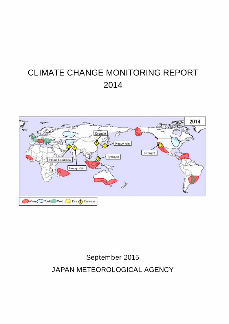
Cover: Extreme events and weather-related disasters observed in 2014 Schematic representation of major extreme climatic events and weather-related disasters occurring during the year. See Section 1.1 for detail.
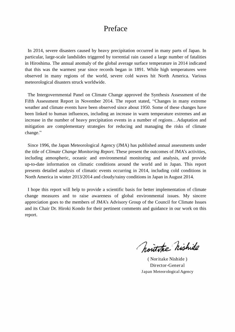
Preface
In 2014, severe disasters caused by heavy precipitation occurred in many parts of Japan. In particular, large-scale landslides triggered by torrential rain caused a large number of fatalities in Hiroshima. The annual anomaly of the global average surface temperature in 2014 indicated that this was the warmest year since records began in 1891. While high temperatures were observed in many regions of the world, severe cold waves hit North America. Various meteorological disasters struck worldwide.
The Intergovernmental Panel on Climate Change approved the Synthesis Assessment of the
Fifth Assessment Report in November 2014. The report stated, “Changes in many extreme weather and climate events have been observed since about 1950. Some of these changes have been linked to human influences, including an increase in warm temperature extremes and an increase in the number of heavy precipitation events in a number of regions…Adaptation and mitigation are complementary strategies for reducing and managing the risks of climate change.”
Since 1996, the Japan Meteorological Agency (JMA) has published annual assessments under
the title of Climate Change Monitoring Report. These present the outcomes of JMA’s activities, including atmospheric, oceanic and environmental monitoring and analysis, and provide up-to-date information on climatic conditions around the world and in Japan. This report presents detailed analysis of climatic events occurring in 2014, including cold conditions in North America in winter 2013/2014 and cloudy/rainy conditions in Japan in August 2014.
I hope this report will help to provide a scientific basis for better implementation of climate
change measures and to raise awareness of global environmental issues. My sincere appreciation goes to the members of JMA’s Advisory Group of the Council for Climate Issues and its Chair Dr. Hiroki Kondo for their pertinent comments and guidance in our work on this report.
( Noritake Nishide )
Director-General Japan Meteorological Agency

Index
Chapter 1 Climate in 2014 ……………………………………………………………… 1 1.1 Global climate summary ………..…………….………………………………….…… 1 1.2 Climate in Japan …………….……..………………………………………………… 4
1.2.1 Annual characteristics ………………………………...…...………………… 4 1.2.2 Seasonal characteristics …………………………...………………………… 5
1.3 Atmospheric circulation and oceanographic conditions ………………………… 8 1.3.1 Characteristics of individual seasons ……….…………………….………… 8 1.3.2 Analysis of specific events occurring in 2014 …………………………… 15
Chapter 2 Climate Change ……………………………………………………………… 19
2.1 Changes in temperature ……………………………………………………..……… 19 2.1.1 Global surface temperature ………………………………………………… 19 2.1.2 Surface temperature over Japan …………………………………………… 21 2.1.3 Long-term trends of extreme temperature events in Japan ………………… 22 2.1.4 Urban heat island effect at urban stations in Japan ………………………… 23
2.2 Changes in precipitation ………………………………………………………….… 25 2.2.1 Global precipitation over land ………………………………………….… 25 2.2.2 Precipitation over Japan …………………………………………………… 25 2.2.3 Snow depth in Japan ………………………………………………………26 2.2.4 Long-term trends of extreme precipitation events in Japan ………….…… 27 2.2.5 Long-term trends of heavy rainfall analyzed using AMeDAS data …..…… 28
2.3 Changes in the phenology of cherry blossoms and acer leaves in Japan …………… 30 2.4 Tropical cyclones …………………………………………………………..……… 31 2.5 Sea surface temperature …………………………………………………………… 32
2.5.1 Global sea surface temperature …………………………………….……… 32 2.5.2 Sea surface temperature (around Japan) …………………………………… 33
2.6 El Niño/La Niña and PDO (Pacific Decadal Oscillation) ………………………… 34 2.6.1 El Niño/La Niña …………………………………………………………… 34 2.6.2 Pacific Decadal Oscillation ……………………………………………… 35
2.7 Global upper ocean heat content …………………………………………………… 36 2.8 Sea levels around Japan …………………………………………………………… 37 2.9 Sea ice ……………………………..………………………………………………… 39
2.9.1 Sea ice in Arctic and Antarctic areas ……………………………………… 39 2.9.2 Sea ice in the Sea of Okhotsk ……………………………………………… 40
2.10 Snow cover in the Northern Hemisphere ……………………………………… 40
Chapter3 Atmospheric and Marine Environment Monitoring ………………………... 42 3.1 Monitoring of greenhouse gases …………………………………………………...... 42
3.1.1 Global and domestic atmospheric carbon dioxide concentrations ……….. 43 [Column] Ocean acidification in the Pacific ……………………………………… 48 3.1.2 Global and domestic atmospheric methane concentrations ……………… 49
3.1.3 Global and domestic atmospheric nitrous oxide concentrations ………… 51
3.2 Monitoring of the ozone layer and ultraviolet radiation …………………………… 53 3.2.1 Global and domestic observation of ozone-depleting substances ………… 53 3.2.2 Ozone layer …………………………………………..…………………… 55 3.2.3 Solar UV radiation in Japan ………………………….…………………… 57
3.3 Monitoring of aerosols and surface radiation ……………………………………… 58 3.3.1 Aerosols …………………………………………………………………… 58 3.3.2 Kosa (Aeolian dust) .…………………...………..………………………… 58 3.3.3 Solar radiation and downward infrared radiation ………………………… 59
Explanatory note on detection of statistical significance in long-term trends …………… 62 Glossary …………………………………………………………...……………………… 64 Map 1 Names of world regions ………………………………………………………...… 68 Map 2 Names of Japan’s island areas and
Names of Japanese regions used in this report ……… 68 Map 3 Distribution of surface meteorological observation stations in Japan ………...…… 69 References …………………………………………………...…………………………… 70

(Chapter 1 Climate in 2014)
1
Chapter 1 Climate in 2014
1.1 Global climate summary ○ Extremely high temperatures were frequently observed in low-latitude areas from June
onward. ○ Extremely low temperatures were frequently observed around the Midwest of the USA,
while extremely high temperatures were observed throughout the year from the southwestern USA to northwestern Mexico. Drought persisted in the southwestern USA.
○ Weather-related disasters were caused by torrential rains in northern Afghanistan (April to June), India (July to September), Nepal (August) and Pakistan (September). Major extreme climate events and weather-related disasters occurring in 2014 are shown in
Figure 1.1-1 and Table 1.1-1. Extremely high temperatures were frequently observed in low-latitude areas in the second
half of the year (see (6), (12), (13) and (18) in Figure 1.1-1). Extremely low temperatures were observed around the Midwest of the USA from January to
March, in July and in November, while extremely high temperatures were observed throughout the year from the southwestern USA to northwestern Mexico (see (15) and (17) in Figure 1.1-1). The three-month mean temperature from January to March in Detroit, Michigan, was -5.8°C (4.9°C lower than the normal), and the annual mean temperature in San Francisco, California, was 16.7°C (2.2°C higher than the normal). Wildfires and agricultural losses caused by the persistent drought in the southwestern USA were reported (see (16) in Figure 1.1-1).
Torrential rains in parts of Japan from 30 July to 26 August caused more than 80 fatalities (see (1) in Figure 1.1-1). In northern Afghanistan, floods and landslides caused more than 750 fatalities from April to June. During the monsoon season from June to September, torrential rains caused more than 1,000 fatalities in India, more than 250 in Nepal and more than 360 in Pakistan.
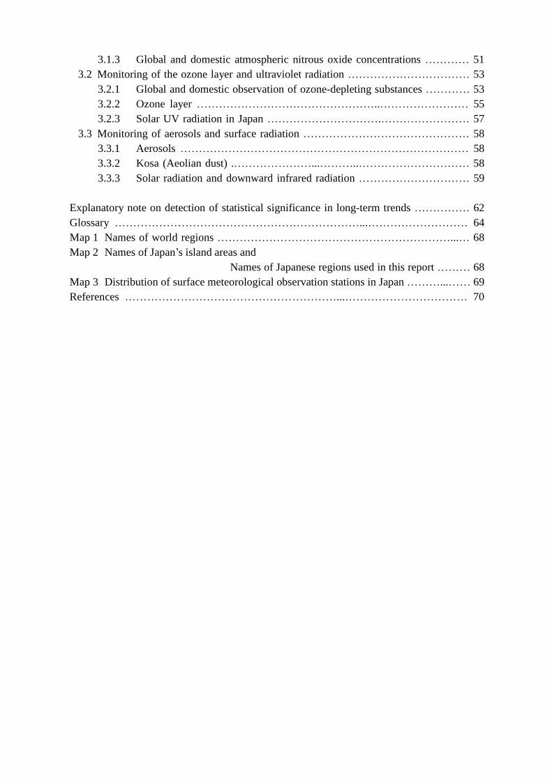
Annual mean temperatures were above normal in many parts of the world, and were below normal in the Philippines, from Western Siberia to Central Asia and from central Canada to the southern USA (Figure 1.1-2).
Annual precipitation amounts were above normal from Central Siberia to the eastern part of Central Asia, on the southern Scandinavian Peninsula, in southeastern Europe, around the Red Sea, in the northeastern USA, in western Mexico, in the southern part of South America and from Micronesia to the southern Philippines, and were below normal on the southern Arabian Peninsula and in southern Algeria (Figure 1.1-3).
(Chapter 1 Climate in 2014)
2
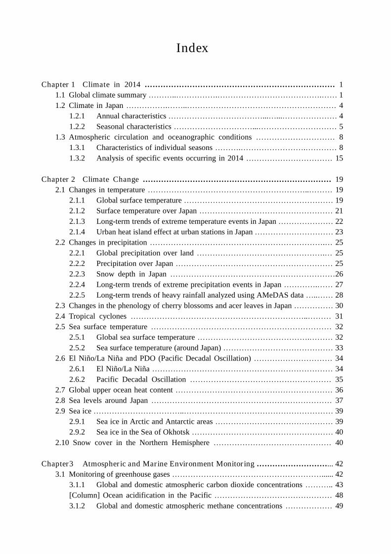
Figure 1.1-1 Extreme events and weather-related disasters observed in 2014
Schematic representation of major extreme climatic events and weather-related disasters occurring during the year.
Table 1.1-1 Extreme events and weather-related disasters occurring in 2014
No. Events
(1) Torrential rain in Japan (August)
(2) Drought in northeastern and eastern China (June − August)
(3) Low temperatures in the southern part of Western Siberia (July, September – October)
(4) Low temperatures in the southern part of Central Asia (February, October – November)
(5) Typhoon in the Philippines (July)
(6) High temperatures from Malaysia to Indonesia (June – July, October – November)
(7) Torrential rain in India, Nepal and Pakistan (July − September)
(8) Floods and Landslides in northern Afghanistan (April − June)
(9) Heavy precipitation in southeastern Europe (May – June, August – September, December)
(10) High temperatures in southern Europe (February, April, October – November)
(11) Heavy precipitation in western Europe (January – February, May, July – August, November)
(12) High temperatures in western Africa (June – July, November)
(13) High temperatures around northern Madagascar (July – August, October – December)
(14) High temperatures in western Alaska (January, August, November)
(15) Low temperatures around the Midwest of the USA (January – March, July, November)
(16) Drought in California (all year round)
(17) High temperatures from the southwestern USA to northwestern Mexico (all year round)
(18) High temperatures around the Caribbean Sea (June – July, November)
(19) High temperatures (January – February, September – October) and heavy precipitation (June – July, September – October) around southern Brazil
(20) High temperatures in southern Australia (May, September – October) Data and information on disasters are based on official reports of the United Nations and national governments and databases of research institutes (EM-DAT).
(Chapter 1 Climate in 2014)
3
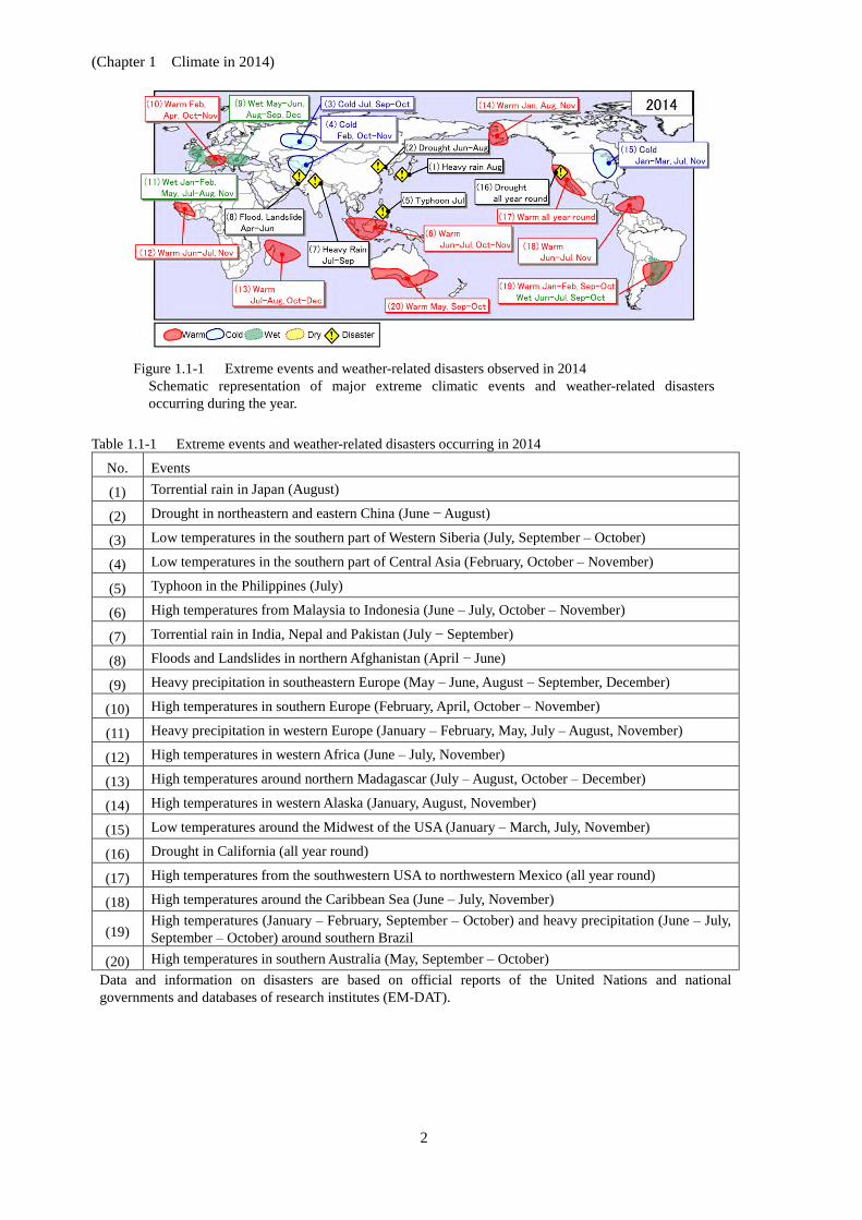
Figure 1.1-2 Annual mean temperature anomalies in 2014
Categories are defined by the annual mean temperature anomaly against the normal divided by its standard deviation and averaged in 5° × 5° grid boxes. Red marks indicate values above the normal calculated from 1981 to 2010, and blue marks indicate values below the normal. The thresholds of each category are –1.28, –0.44, 0, +0.44 and +1.281. Areas over land without graphical marks are those where observation data are insufficient or where normal data are unavailable.
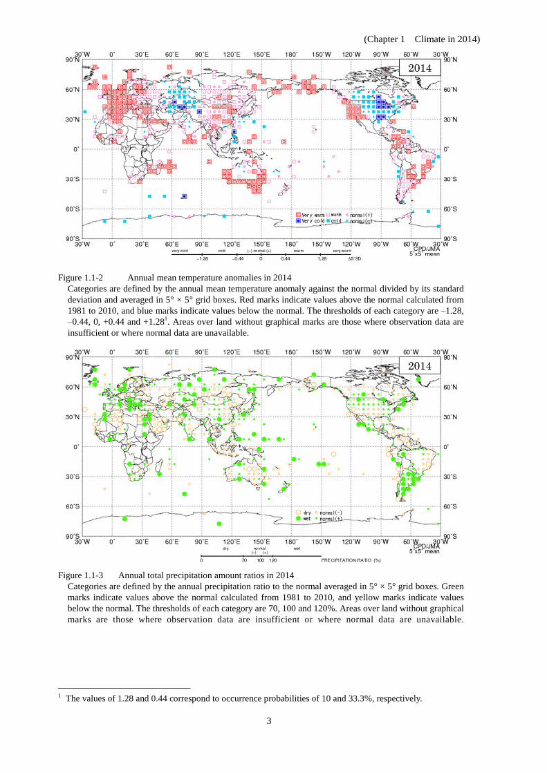
Figure 1.1-3 Annual total precipitation amount ratios in 2014
Categories are defined by the annual precipitation ratio to the normal averaged in 5° × 5° grid boxes. Green marks indicate values above the normal calculated from 1981 to 2010, and yellow marks indicate values below the normal. The thresholds of each category are 70, 100 and 120%. Areas over land without graphical marks are those where observation data are insufficient or where normal data are unavailable.
1 The values of 1.28 and 0.44 correspond to occurrence probabilities of 10 and 33.3%, respectively.
(Chapter 1 Climate in 2014)
4
1.2 Climate in Japan2 ○ Annual sunshine durations were significantly above normal on the Pacific side of northern
Japan and in eastern Japan in conjunction with dominant migratory high-pressure systems. These conditions brought sunny weather to northern and eastern Japan in spring and autumn.
○ Western Japan experienced a cool and wet summer for the first time since 2003 due to weaker-than-normal northwestward expansion of the Pacific High.
○ Two record-breaking heavy snowfall events hit the Kanto/Koshin region of eastern Japan in February.
○ Hazardous extremely heavy rains were observed nationwide due to active fronts and typhoons from late July to August.
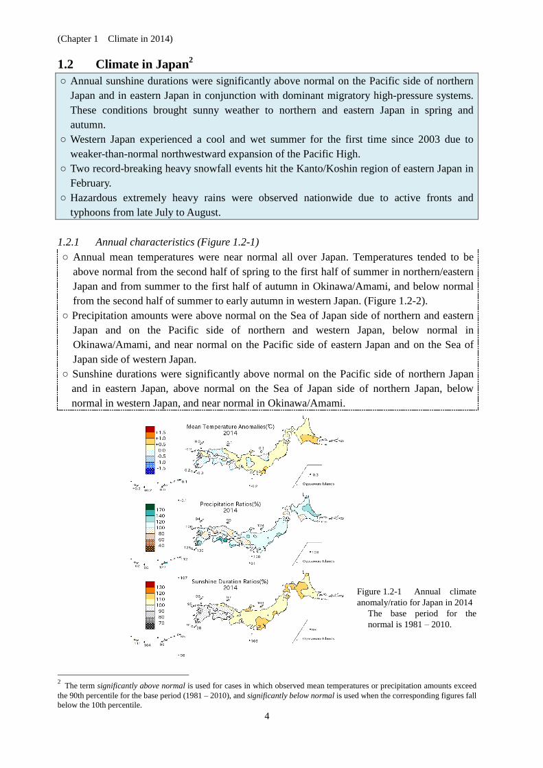
1.2.1 Annual characteristics (Figure 1.2-1) ○ Annual mean temperatures were near normal all over Japan. Temperatures tended to be
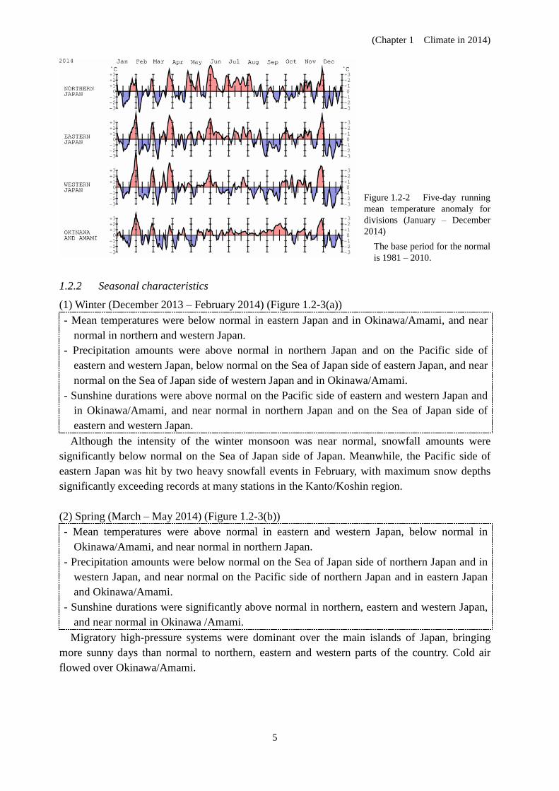
above normal from the second half of spring to the first half of summer in northern/eastern Japan and from summer to the first half of autumn in Okinawa/Amami, and below normal from the second half of summer to early autumn in western Japan. (Figure 1.2-2).
○ Precipitation amounts were above normal on the Sea of Japan side of northern and eastern Japan and on the Pacific side of northern and western Japan, below normal in Okinawa/Amami, and near normal on the Pacific side of eastern Japan and on the Sea of Japan side of western Japan.
○ Sunshine durations were significantly above normal on the Pacific side of northern Japan and in eastern Japan, above normal on the Sea of Japan side of northern Japan, below normal in western Japan, and near normal in Okinawa/Amami.
Figure 1.2-1 Annual climate anomaly/ratio for Japan in 2014
The base period for the normal is 1981 – 2010.
2 The term significantly above normal is used for cases in which observed mean temperatures or precipitation amounts exceed the 90th percentile for the base period (1981 – 2010), and significantly below normal is used when the corresponding figures fall below the 10th percentile.
(Chapter 1 Climate in 2014)
5
Figure 1.2-2 Five-day running mean temperature anomaly for divisions (January – December 2014)
The base period for the normal is 1981 – 2010.
1.2.2 Seasonal characteristics
(1) Winter (December 2013 – February 2014) (Figure 1.2-3(a)) - Mean temperatures were below normal in eastern Japan and in Okinawa/Amami, and near
normal in northern and western Japan. - Precipitation amounts were above normal in northern Japan and on the Pacific side of
eastern and western Japan, below normal on the Sea of Japan side of eastern Japan, and near normal on the Sea of Japan side of western Japan and in Okinawa/Amami.
- Sunshine durations were above normal on the Pacific side of eastern and western Japan and in Okinawa/Amami, and near normal in northern Japan and on the Sea of Japan side of eastern and western Japan.
Although the intensity of the winter monsoon was near normal, snowfall amounts were significantly below normal on the Sea of Japan side of Japan. Meanwhile, the Pacific side of eastern Japan was hit by two heavy snowfall events in February, with maximum snow depths significantly exceeding records at many stations in the Kanto/Koshin region.
(2) Spring (March – May 2014) (Figure 1.2-3(b)) - Mean temperatures were above normal in eastern and western Japan, below normal in
Okinawa/Amami, and near normal in northern Japan. - Precipitation amounts were below normal on the Sea of Japan side of northern Japan and in
western Japan, and near normal on the Pacific side of northern Japan and in eastern Japan and Okinawa/Amami.
- Sunshine durations were significantly above normal in northern, eastern and western Japan, and near normal in Okinawa /Amami.
Migratory high-pressure systems were dominant over the main islands of Japan, bringing more sunny days than normal to northern, eastern and western parts of the country. Cold air flowed over Okinawa/Amami.
(Chapter 1 Climate in 2014)
6
(3) Summer (June – August 2014) (Figure 1.2-3(c)) - Mean temperatures were above normal in northern and eastern Japan and in
Okinawa/Amami, and below normal in western Japan. - Precipitation amounts were significantly above normal in northern Japan and on the Pacific
side of western Japan, above normal on the Sea of Japan side of eastern and western Japan, and near normal on the Pacific side of eastern Japan and in Okinawa/Amami.
- Sunshine durations were significantly below normal in western Japan, below normal on the Sea of Japan side of eastern Japan and in Okinawa/Amami, above normal on the Sea of Japan side of northern Japan, and near normal on the Pacific side of northern and eastern Japan.
Due to weaker-than-normal northwestward expansion of the Pacific High, western Japan experienced a cool summer for the first time since 2003, and the sunshine duration total for the Pacific side of western Japan was the lowest for August since 1946. Hazardous extremely heavy rains were observed nationwide due to active fronts and typhoons from late July to August.
(4) Autumn (September – November 2014) (Figure 1.2-3(d)) - Mean temperatures were significantly above normal in Okinawa/Amami, and near normal in
northern, eastern and western Japan. - Precipitation amounts were below normal in northern Japan and Okinawa/Amami, and near
normal in eastern and western Japan. - Sunshine durations were significantly above normal in northern Japan and on the Sea of
Japan side of eastern Japan, and above normal on the Pacific side of eastern Japan and in Okinawa/Amami.
Migratory high-pressure systems were dominant over the Tohoku region of northern Japan and the Hokuriku region on the Sea of Japan side of eastern Japan, bringing the highest sunshine durations since 1946 to the Sea of Japan side of eastern Japan. The enhanced Pacific High covered the Sakishima Islands of southwestern Japan, bringing hot and dry conditions to the area from the second half of summer to the first half of autumn. (5) Early Winter (December 2014)
In conjunction with a stronger-than-normal winter monsoon pattern, monthly mean temperatures were below normal nationwide. Snowfall amounts were above normal on the Sea of Japan side of the country. On the same side of northern and eastern Japan, monthly precipitation amounts were the highest on record for December since 1946 due to cold surges and cyclones frequently passing near the country.
(Chapter 1 Climate in 2014)
7
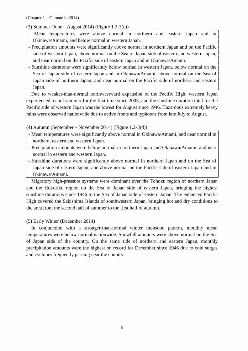
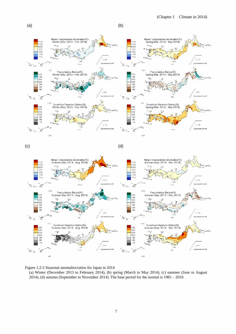
(a) (b)
(c) (d)
Figure 1.2-3 Seasonal anomalies/ratios for Japan in 2014 (a) Winter (December 2013 to February 2014), (b) spring (March to May 2014), (c) summer (June to August 2014), (d) autumn (September to November 2014). The base period for the normal is 1981 – 2010.

(Chapter 1 Climate in 2014)
8
1.3 Atmospheric circulation and oceanographic conditions3
○ In winter, central to eastern North America was repeatedly affected by harsh cold waves associated with the Arctic cold air mass sitting more toward North America than normal and significant southward meandering of the jet stream.
○ In August, western Japan experienced record-high precipitation and a record-low sunshine duration, primarily due to two typhoons approaching and making landfall in rapid succession in combination with a stationary front and sustained inflow of moist air associated with the jet stream meandering and flowing south of its normal position.
○ Although El Niño conditions emerged in summer and continued thereafter, global atmospheric circulation did not resemble that of a typical El Niño episode. Monitoring of atmospheric and oceanographic conditions (e.g., upper air flow, tropical
convective activity and sea surface temperatures (SSTs)) is key to understanding the causes of extreme weather events4 . This section briefly outlines the characteristics of atmospheric circulation and oceanographic conditions seen in 2014. 1.3.1 Characteristics of individual seasons5 (1) Winter (December 2013 – February 2014)6
SSTs were above normal in western parts of the equatorial Pacific and below normal in central to eastern parts (Figure 1.3-1). In association with these conditions, tropical convective activity was enhanced over the area from Indonesia to the western equatorial Pacific, and was suppressed over the central equatorial Pacific (Figure 1.3-2).
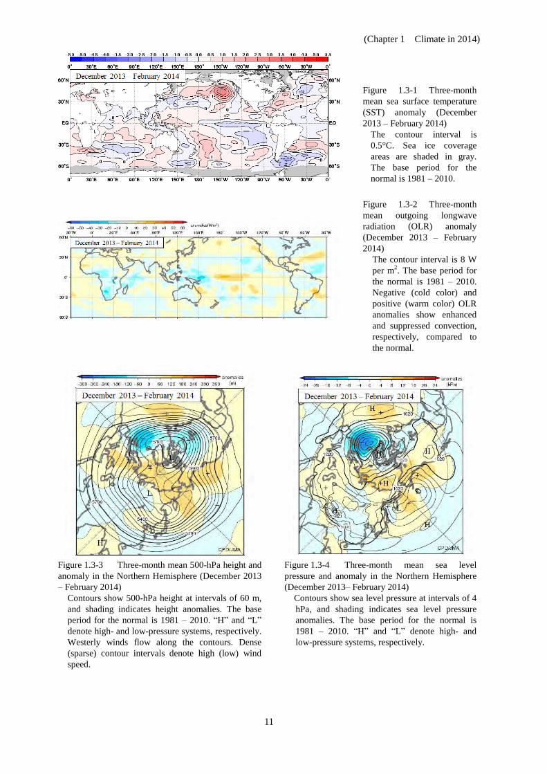
In the 500-hPa height field, positive anomalies were seen over the Arctic region and negative anomalies were seen across central to eastern North America (Figure 1.3-3), indicating above-normal inflow of the Arctic cold air mass into central to eastern North America. This led to repeated cold waves and severe impacts on socio-economic activity in the region. An anticyclone centered on the southwest of the USA was stronger than normal in its northward extension, causing northerly winds to be dominant and southerly moist winds to be suppressed over the southwestern USA and resulting in drier-than-normal conditions there. Meanwhile, distinctive negative anomalies and equatorward-protruding 500-hPa height contours were observed to the west of Europe, indicating the persistence of an upper-tropospheric trough. In association, numerous extratropical cyclones formed and developed to the west of Europe (Figure 1.3.4), bringing wetter-than-normal winter conditions to the UK and France. (2) Spring (March – May 2014) 3 See the Glossary for terms relating to El Niño phenomena, monsoons and Arctic Oscillation. 4 The main charts used for monitoring of atmospheric circulation and oceanographic conditions are: sea surface temperature
(SST) maps representing SST distribution for monitoring of oceanographic variability elements such as El Niño/La Niña phenomena; outgoing longwave radiation (OLR) maps representing the strength of longwave radiation from the earth’s surface under clear sky conditions into space or from the top of clouds under cloudy conditions into space for monitoring of convective activity; 500-hPa height maps representing air flow at a height of approximately 5,000 meters for monitoring of atmospheric circulation variability elements such as westerly jet streams and the Arctic Oscillation; and sea level pressure maps representing air flow and pressure systems on the earth’s surface for monitoring of the Pacific High, the Siberian High, the Arctic Oscillation and other phenomena.
5 JMA publishes Monthly Highlights on the Climate System including information on the characteristics of climatic anomalies and extreme events around the world, atmospheric circulation and oceanographic conditions. It can be found at http://ds.data.jma.go.jp/tcc/tcc/products/clisys/highlights/index.html.
6 See Section 1.3.2 (1) for details of cold conditions over Japan and northern East Asia.
(Chapter 1 Climate in 2014)
9
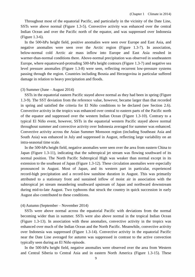
Throughout most of the equatorial Pacific, and particularly in the vicinity of the Date Line, SSTs were above normal (Figure 1.3-5). Convective activity was enhanced over the central Indian Ocean and over the Pacific north of the equator, and was suppressed over Indonesia (Figure 1.3-6).
In the 500-hPa height field, positive anomalies were seen over Europe and East Asia, and negative anomalies were seen over the Arctic region (Figure 1.3-7). In association, below-normal cold Arctic air mass inflow into Europe and East Asia resulted in warmer-than-normal conditions there. Above-normal precipitation was observed in southeastern Europe, where equatorward-protruding 500-hPa height contours (Figure 1.3-7) and negative sea level pressure anomalies (Figure 1.3-8) were seen, reflecting recurrent low-pressure systems passing through the region. Countries including Bosnia and Herzegovina in particular suffered damage in relation to heavy precipitation and floods. (3) Summer (June – August 2014)
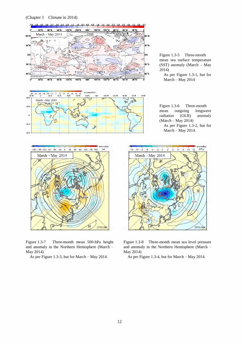
SSTs in the equatorial eastern Pacific stayed above normal as they had been in spring (Figure 1.3-9). The SST deviation from the reference value, however, became larger than that recorded in spring and satisfied the criteria for El Niño conditions to be declared (see Section 2.6). Convective activity in the tropics was enhanced over central to eastern parts of the Pacific north of the equator and suppressed over the western Indian Ocean (Figure 1.3-10). Contrary to a typical El Niño event, however, SSTs in the equatorial western Pacific stayed above normal throughout summer and convective activity over Indonesia averaged for summer was enhanced. Convective activity across the Asian Summer Monsoon region (including Southeast Asia and South Asia) was enhanced in July and suppressed in August, reflecting large variability on an intra-seasonal time scale.
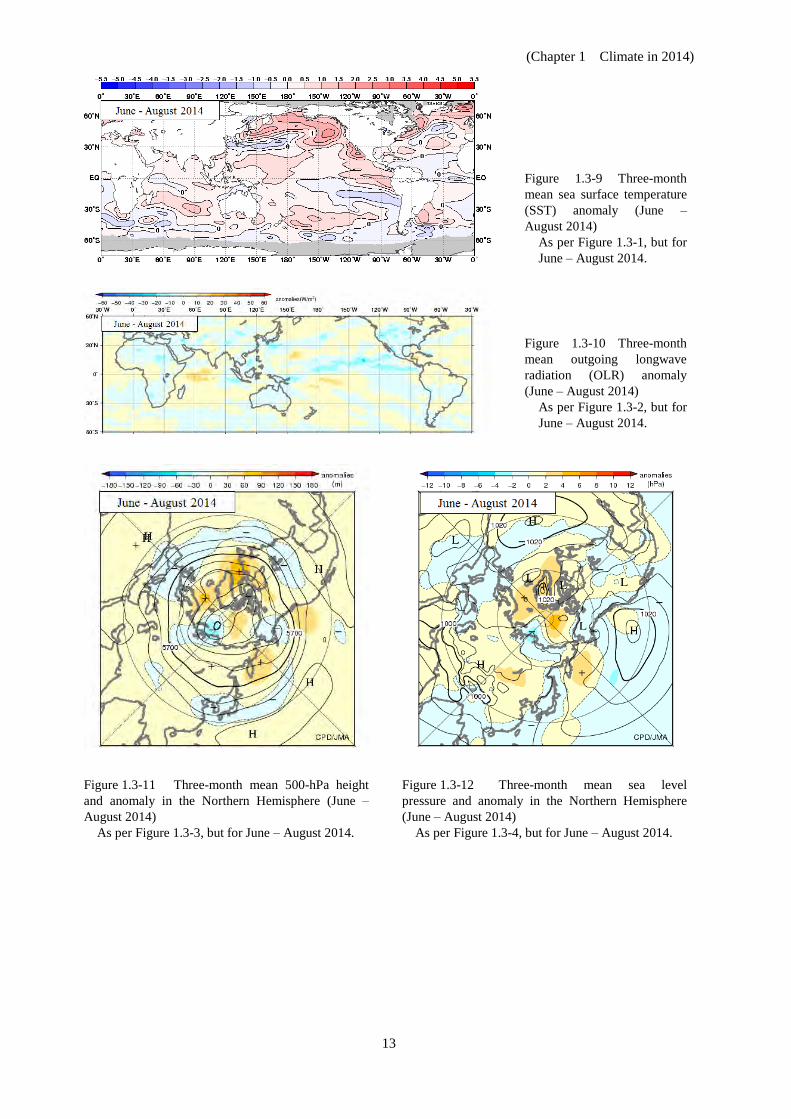
In the 500-hPa height field, negative anomalies were seen over the area from eastern China to Japan (Figure 1.3-11), indicating that the subtropical jet stream was flowing southward of its normal position. The North Pacific Subtropical High was weaker than normal except in its extension to the southeast of Japan (Figure 1.3-12). These circulation anomalies were especially pronounced in August. Most of Japan, and its western part in particular, experienced record-high precipitation and a record-low sunshine duration in August. This was primarily attributed to a stationary front and sustained inflow of moist air in association with the subtropical jet stream meandering southward upstream of Japan and northward downstream during mid-to-late August. Two typhoons that struck the country in quick succession in early August also contributed to these conditions. (4) Autumn (September – November 2014)
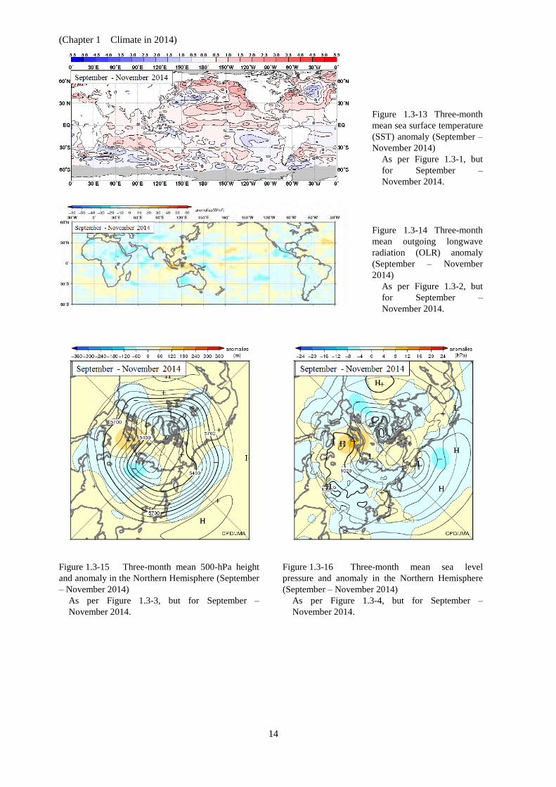
SSTs were above normal across the equatorial Pacific with deviations from the normal becoming wider than in summer. SSTs were also above normal in the tropical Indian Ocean (Figure 1.3-13). In association with these anomalies, convective activity in the tropics was enhanced over much of the Indian Ocean and the North Pacific. Meanwhile, convective activity over Indonesia was suppressed (Figure 1.3-14). Convective activity in the equatorial Pacific near the Date Line averaged for autumn was suppressed in contrast to the active convection typically seen during an El Niño episode.
In the 500-hPa height field, negative anomalies were observed over the area from Western and Central Siberia to Central Asia and in eastern North America (Figure 1.3-15). These

(Chapter 1 Climate in 2014)
10
anomalies indicate southward meandering of the jet stream, bringing above-normal inflow of the Arctic cold air mass. Equatorward-protruding 500-hPa height contours (Figure 1.3-15) and negative sea level pressure anomalies (Figure 1.3-16) were seen to the west of Europe. These anomalies were pronounced in November when recurrent extratropical cyclones influenced and brought above-normal precipitation to southwestern Europe.
(Chapter 1 Climate in 2014)
11
Figure 1.3-1 Three-month mean sea surface temperature (SST) anomaly (December 2013 – February 2014)
The contour interval is 0.5°C. Sea ice coverage areas are shaded in gray. The base period for the normal is 1981 – 2010.
Figure 1.3-2 Three-month mean outgoing longwave radiation (OLR) anomaly (December 2013 – February 2014)
The contour interval is 8 W per m2. The base period for the normal is 1981 – 2010. Negative (cold color) and positive (warm color) OLR anomalies show enhanced and suppressed convection, respectively, compared to the normal.
Figure 1.3-3 Three-month mean 500-hPa height and anomaly in the Northern Hemisphere (December 2013 – February 2014)
Contours show 500-hPa height at intervals of 60 m, and shading indicates height anomalies. The base period for the normal is 1981 – 2010. “H” and “L” denote high- and low-pressure systems, respectively. Westerly winds flow along the contours. Dense (sparse) contour intervals denote high (low) wind speed.
Figure 1.3-4 Three-month mean sea level pressure and anomaly in the Northern Hemisphere (December 2013– February 2014)
Contours show sea level pressure at intervals of 4 hPa, and shading indicates sea level pressure anomalies. The base period for the normal is 1981 – 2010. “H” and “L” denote high- and low-pressure systems, respectively.
(Chapter 1 Climate in 2014)
12
Figure 1.3-5 Three-month mean sea surface temperature (SST) anomaly (March – May 2014)
As per Figure 1.3-1, but for March – May 2014
Figure 1.3-6 Three-month mean outgoing longwave radiation (OLR) anomaly (March – May 2014)
As per Figure 1.3-2, but for March – May 2014.
Figure 1.3-7 Three-month mean 500-hPa height and anomaly in the Northern Hemisphere (March – May 2014)
As per Figure 1.3-3, but for March – May 2014.
Figure 1.3-8 Three-month mean sea level pressure and anomaly in the Northern Hemisphere (March – May 2014)
As per Figure 1.3-4, but for March – May 2014.
(Chapter 1 Climate in 2014)
13
Figure 1.3-9 Three-month mean sea surface temperature (SST) anomaly (June – August 2014)
As per Figure 1.3-1, but for June – August 2014.
Figure 1.3-10 Three-month mean outgoing longwave radiation (OLR) anomaly (June – August 2014)
As per Figure 1.3-2, but for June – August 2014.
Figure 1.3-11 Three-month mean 500-hPa height and anomaly in the Northern Hemisphere (June – August 2014)
As per Figure 1.3-3, but for June – August 2014.
Figure 1.3-12 Three-month mean sea level pressure and anomaly in the Northern Hemisphere (June – August 2014)
As per Figure 1.3-4, but for June – August 2014.
(Chapter 1 Climate in 2014)
14
Figure 1.3-13 Three-month mean sea surface temperature (SST) anomaly (September – November 2014)
As per Figure 1.3-1, but for September – November 2014.
Figure 1.3-14 Three-month mean outgoing longwave radiation (OLR) anomaly (September – November 2014)
As per Figure 1.3-2, but for September – November 2014.
Figure 1.3-15 Three-month mean 500-hPa height and anomaly in the Northern Hemisphere (September – November 2014)
As per Figure 1.3-3, but for September – November 2014.
Figure 1.3-16 Three-month mean sea level pressure and anomaly in the Northern Hemisphere (September – November 2014)
As per Figure 1.3-4, but for September – November 2014.
(Chapter 1 Climate in 2014)
15
1.3.2 Analysis of specific events occurring in 20147 (1) Winter 2013/2014 cold waves over North America8
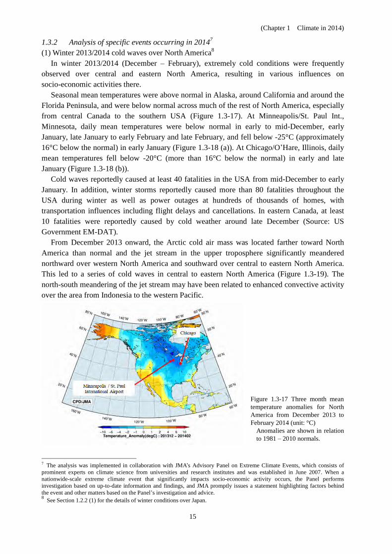
In winter 2013/2014 (December – February), extremely cold conditions were frequently observed over central and eastern North America, resulting in various influences on socio-economic activities there.
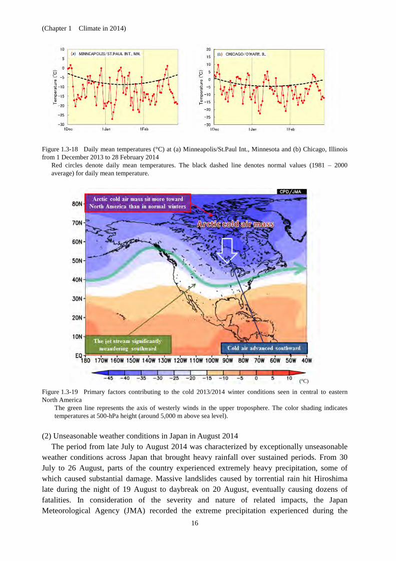
Seasonal mean temperatures were above normal in Alaska, around California and around the Florida Peninsula, and were below normal across much of the rest of North America, especially from central Canada to the southern USA (Figure 1.3-17). At Minneapolis/St. Paul Int., Minnesota, daily mean temperatures were below normal in early to mid-December, early January, late January to early February and late February, and fell below -25°C (approximately 16°C below the normal) in early January (Figure 1.3-18 (a)). At Chicago/O’Hare, Illinois, daily mean temperatures fell below -20°C (more than 16°C below the normal) in early and late January (Figure 1.3-18 (b)).
Cold waves reportedly caused at least 40 fatalities in the USA from mid-December to early January. In addition, winter storms reportedly caused more than 80 fatalities throughout the USA during winter as well as power outages at hundreds of thousands of homes, with transportation influences including flight delays and cancellations. In eastern Canada, at least 10 fatalities were reportedly caused by cold weather around late December (Source: US Government EM-DAT).
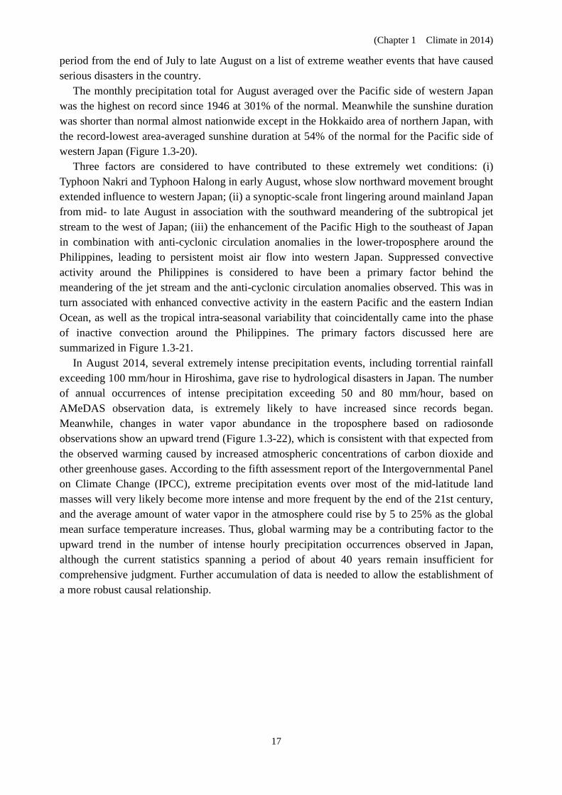
From December 2013 onward, the Arctic cold air mass was located farther toward North America than normal and the jet stream in the upper troposphere significantly meandered northward over western North America and southward over central to eastern North America. This led to a series of cold waves in central to eastern North America (Figure 1.3-19). The north-south meandering of the jet stream may have been related to enhanced convective activity over the area from Indonesia to the western Pacific.
Figure 1.3-17 Three month mean temperature anomalies for North America from December 2013 to February 2014 (unit: °C)
Anomalies are shown in relation to 1981 – 2010 normals.
7 The analysis was implemented in collaboration with JMA’s Advisory Panel on Extreme Climate Events, which consists of prominent experts on climate science from universities and research institutes and was established in June 2007. When a nationwide-scale extreme climate event that significantly impacts socio-economic activity occurs, the Panel performs investigation based on up-to-date information and findings, and JMA promptly issues a statement highlighting factors behind the event and other matters based on the Panel’s investigation and advice. 8 See Section 1.2.2 (1) for the details of winter conditions over Japan.
(Chapter 1 Climate in 2014)
16
Figure 1.3-19 Primary factors contributing to the cold 2013/2014 winter conditions seen in central to eastern North America
The green line represents the axis of westerly winds in the upper troposphere. The color shading indicates temperatures at 500-hPa height (around 5,000 m above sea level).
(2) Unseasonable weather conditions in Japan in August 2014
The period from late July to August 2014 was characterized by exceptionally unseasonable weather conditions across Japan that brought heavy rainfall over sustained periods. From 30 July to 26 August, parts of the country experienced extremely heavy precipitation, some of which caused substantial damage. Massive landslides caused by torrential rain hit Hiroshima late during the night of 19 August to daybreak on 20 August, eventually causing dozens of fatalities. In consideration of the severity and nature of related impacts, the Japan Meteorological Agency (JMA) recorded the extreme precipitation experienced during the
Figure 1.3-18 Daily mean temperatures (°C) at (a) Minneapolis/St.Paul Int., Minnesota and (b) Chicago, Illinois from 1 December 2013 to 28 February 2014
Red circles denote daily mean temperatures. The black dashed line denotes normal values (1981 – 2000 average) for daily mean temperature.
(°C)
(Chapter 1 Climate in 2014)
17
period from the end of July to late August on a list of extreme weather events that have caused serious disasters in the country.
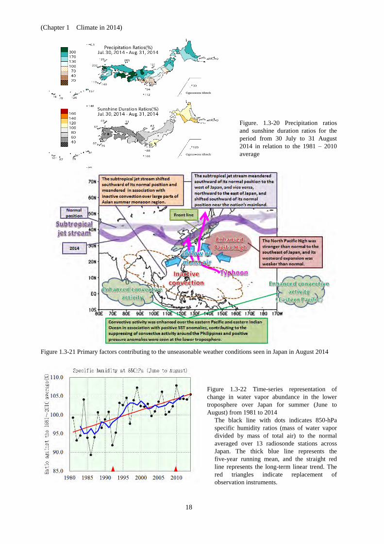
The monthly precipitation total for August averaged over the Pacific side of western Japan was the highest on record since 1946 at 301% of the normal. Meanwhile the sunshine duration was shorter than normal almost nationwide except in the Hokkaido area of northern Japan, with the record-lowest area-averaged sunshine duration at 54% of the normal for the Pacific side of western Japan (Figure 1.3-20).
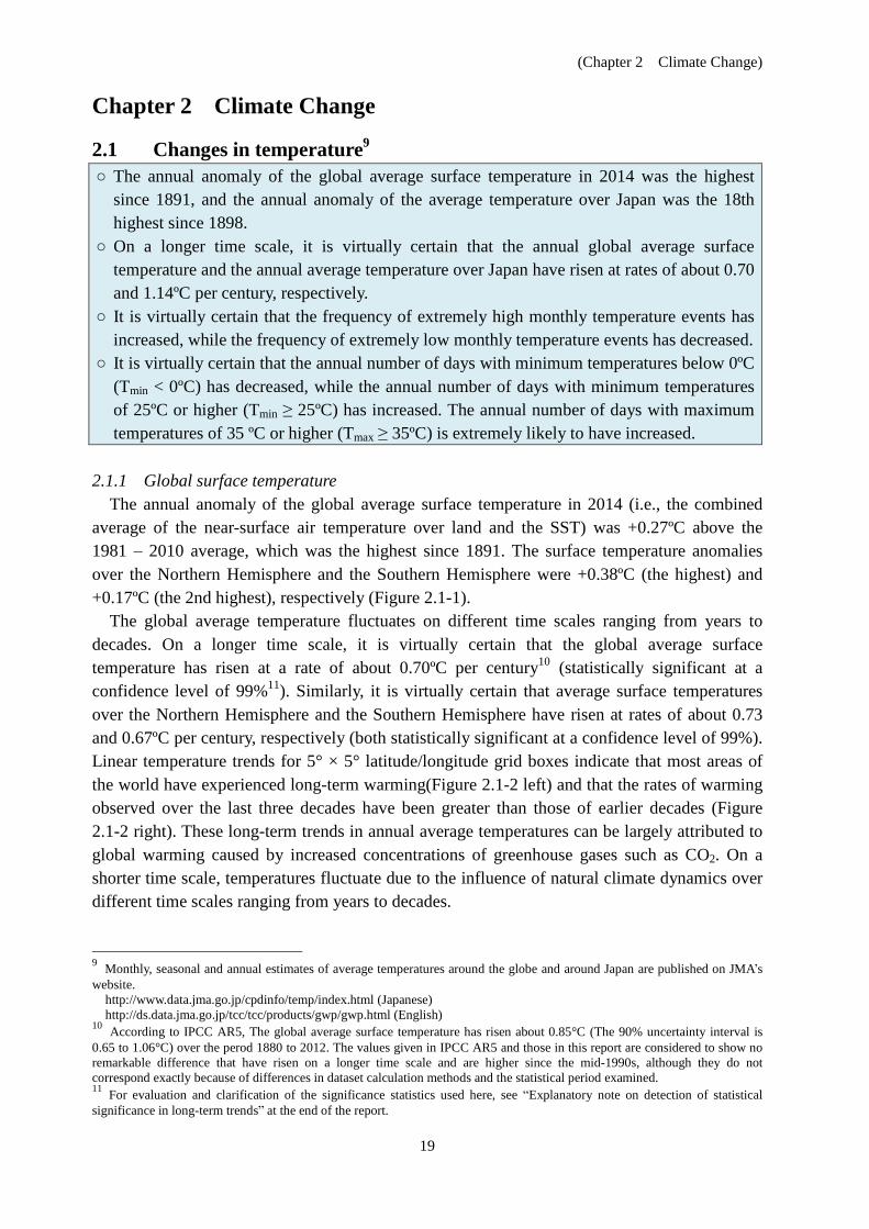
Three factors are considered to have contributed to these extremely wet conditions: (i) Typhoon Nakri and Typhoon Halong in early August, whose slow northward movement brought extended influence to western Japan; (ii) a synoptic-scale front lingering around mainland Japan from mid- to late August in association with the southward meandering of the subtropical jet stream to the west of Japan; (iii) the enhancement of the Pacific High to the southeast of Japan in combination with anti-cyclonic circulation anomalies in the lower-troposphere around the Philippines, leading to persistent moist air flow into western Japan. Suppressed convective activity around the Philippines is considered to have been a primary factor behind the meandering of the jet stream and the anti-cyclonic circulation anomalies observed. This was in turn associated with enhanced convective activity in the eastern Pacific and the eastern Indian Ocean, as well as the tropical intra-seasonal variability that coincidentally came into the phase of inactive convection around the Philippines. The primary factors discussed here are summarized in Figure 1.3-21.
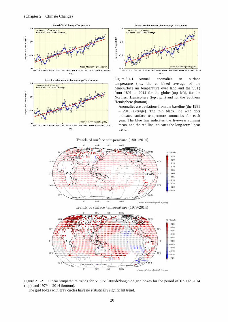
In August 2014, several extremely intense precipitation events, including torrential rainfall exceeding 100 mm/hour in Hiroshima, gave rise to hydrological disasters in Japan. The number of annual occurrences of intense precipitation exceeding 50 and 80 mm/hour, based on AMeDAS observation data, is extremely likely to have increased since records began. Meanwhile, changes in water vapor abundance in the troposphere based on radiosonde observations show an upward trend (Figure 1.3-22), which is consistent with that expected from the observed warming caused by increased atmospheric concentrations of carbon dioxide and other greenhouse gases. According to the fifth assessment report of the Intergovernmental Panel on Climate Change (IPCC), extreme precipitation events over most of the mid-latitude land masses will very likely become more intense and more frequent by the end of the 21st century, and the average amount of water vapor in the atmosphere could rise by 5 to 25% as the global mean surface temperature increases. Thus, global warming may be a contributing factor to the upward trend in the number of intense hourly precipitation occurrences observed in Japan, although the current statistics spanning a period of about 40 years remain insufficient for comprehensive judgment. Further accumulation of data is needed to allow the establishment of a more robust causal relationship.
(Chapter 1 Climate in 2014)
18
Figure. 1.3-20 Precipitation ratios and sunshine duration ratios for the period from 30 July to 31 August 2014 in relation to the 1981 – 2010 average
Figure 1.3-21 Primary factors contributing to the unseasonable weather conditions seen in Japan in August 2014
Figure 1.3-22 Time-series representation of change in water vapor abundance in the lower troposphere over Japan for summer (June to August) from 1981 to 2014
The black line with dots indicates 850-hPa specific humidity ratios (mass of water vapor divided by mass of total air) to the normal averaged over 13 radiosonde stations across Japan. The thick blue line represents the five-year running mean, and the straight red line represents the long-term linear trend. The red triangles indicate replacement of observation instruments.
(Chapter 2 Climate Change)
19
Chapter 2 Climate Change
2.1 Changes in temperature9 ○ The annual anomaly of the global average surface temperature in 2014 was the highest
since 1891, and the annual anomaly of the average temperature over Japan was the 18th highest since 1898.
○ On a longer time scale, it is virtually certain that the annual global average surface temperature and the annual average temperature over Japan have risen at rates of about 0.70 and 1.14ºC per century, respectively.
○ It is virtually certain that the frequency of extremely high monthly temperature events has increased, while the frequency of extremely low monthly temperature events has decreased.
○ It is virtually certain that the annual number of days with minimum temperatures below 0ºC (Tmin < 0ºC) has decreased, while the annual number of days with minimum temperatures of 25ºC or higher (Tmin ≥ 25ºC) has increased. The annual number of days with maximum temperatures of 35 ºC or higher (Tmax ≥ 35ºC) is extremely likely to have increased.
2.1.1 Global surface temperature
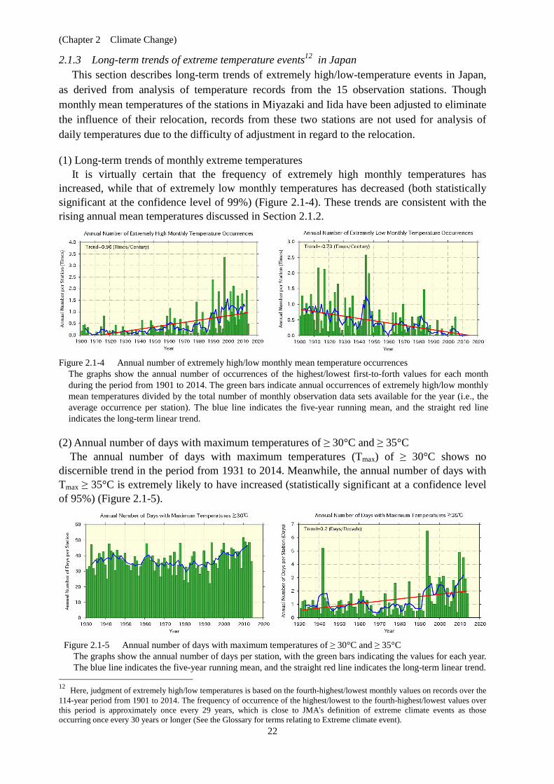
The annual anomaly of the global average surface temperature in 2014 (i.e., the combined average of the near-surface air temperature over land and the SST) was +0.27ºC above the 1981 – 2010 average, which was the highest since 1891. The surface temperature anomalies over the Northern Hemisphere and the Southern Hemisphere were +0.38ºC (the highest) and +0.17ºC (the 2nd highest), respectively (Figure 2.1-1).
The global average temperature fluctuates on different time scales ranging from years to decades. On a longer time scale, it is virtually certain that the global average surface temperature has risen at a rate of about 0.70ºC per century10 (statistically significant at a confidence level of 99%11). Similarly, it is virtually certain that average surface temperatures over the Northern Hemisphere and the Southern Hemisphere have risen at rates of about 0.73 and 0.67ºC per century, respectively (both statistically significant at a confidence level of 99%). Linear temperature trends for 5° × 5° latitude/longitude grid boxes indicate that most areas of the world have experienced long-term warming(Figure 2.1-2 left) and that the rates of warming observed over the last three decades have been greater than those of earlier decades (Figure 2.1-2 right). These long-term trends in annual average temperatures can be largely attributed to global warming caused by increased concentrations of greenhouse gases such as CO2. On a shorter time scale, temperatures fluctuate due to the influence of natural climate dynamics over different time scales ranging from years to decades.
9 Monthly, seasonal and annual estimates of average temperatures around the globe and around Japan are published on JMA’s website.
http://www.data.jma.go.jp/cpdinfo/temp/index.html (Japanese) http://ds.data.jma.go.jp/tcc/tcc/products/gwp/gwp.html (English)
10 According to IPCC AR5, The global average surface temperature has risen about 0.85°C (The 90% uncertainty interval is 0.65 to 1.06°C) over the perod 1880 to 2012. The values given in IPCC AR5 and those in this report are considered to show no remarkable difference that have risen on a longer time scale and are higher since the mid-1990s, although they do not correspond exactly because of differences in dataset calculation methods and the statistical period examined. 11 For evaluation and clarification of the significance statistics used here, see “Explanatory note on detection of statistical significance in long-term trends” at the end of the report.
(Chapter 2 Climate Change)
20
Figure 2.1-1 Annual anomalies in surface temperature (i.e., the combined average of the near-surface air temperature over land and the SST) from 1891 to 2014 for the globe (top left), for the Northern Hemisphere (top right) and for the Southern Hemisphere (bottom).
Anomalies are deviations from the baseline (the 1981 – 2010 average). The thin black line with dots indicates surface temperature anomalies for each year. The blue line indicates the five-year running mean, and the red line indicates the long-term linear trend.
Figure 2.1-2 Linear temperature trends for 5° × 5° latitude/longitude grid boxes for the period of 1891 to 2014 (top), and 1979 to 2014 (bottom).
The grid boxes with gray circles have no statistically significant trend.

(Chapter 2 Climate Change)
21
2.1.2 Surface temperature over Japan Long-term changes in the surface temperature over Japan are analyzed using observational
records dating back to 1898. Table 2.1-1 lists the meteorological stations whose data are used to derive annual mean surface temperatures.
Table 2.1-1 Observation stations whose data are used to calculate surface temperature anomalies over Japan
Miyazaki and Iida were relocated in May 2000 and May 2002, respectively, and their temperatures have been adjusted to eliminate the influence of the relocation.
Element Observation stations
Temperature (15 stations)
Abashiri, Nemuro, Suttsu, Yamagata, Ishinomaki, Fushiki, Iida, Choshi, Sakai, Hamada, Hikone, Miyazaki, Tadotsu, Naze, Ishigakijima
The mean surface temperature in Japan for 2014 is estimated to have been 0.14ºC above the
1981 – 2010 average, which is the 18th warmest on record since 1898 (Figure 2.1-3). The surface temperature fluctuates on different time scales ranging from years to decades. On a longer time scale, it is virtually certain that the annual mean surface temperature over Japan has risen at a rate of about 1.14ºC per century (statistically significant at a confidence level of 99%). Similarly, it is virtually certain that the seasonal mean temperatures for winter, spring, summer and autumn have risen at rates of about 1.08, 1.29, 1.06 and 1.19ºC per century, respectively (all statistically significant at a confidence level of 99%).
It is noticeable from Figure 2.1-3 that the annual mean temperature remained relatively low before the 1940s, started to rise and reached a local peak around 1960, entered a cooler era through to the mid-1980s and then began to show a rapid warming trend in the late 1980s. The warmest years on record have all been observed since the 1990s.
The high temperatures seen in recent years have been influenced by fluctuations over different time scales ranging from years to decades, as well as by global warming resulting from increased concentrations of greenhouse gases such as CO2. This trend is similar to that of worldwide temperatures, as described in Section 2.1.1.
Figure 2.1-3 Annual surface temperature anomalies from 1898 to 2014 in Japan.
Anomalies are deviations from the baseline (the 1981 – 2010 average). The thin black line indicates the surface temperature anomaly for each year. The blue line indicates the five-year running mean, and the red line indicates the long-term linear trend.
(Chapter 2 Climate Change)
22
2.1.3 Long-term trends of extreme temperature events12 in Japan This section describes long-term trends of extremely high/low-temperature events in Japan,
as derived from analysis of temperature records from the 15 observation stations. Though monthly mean temperatures of the stations in Miyazaki and Iida have been adjusted to eliminate the influence of their relocation, records from these two stations are not used for analysis of daily temperatures due to the difficulty of adjustment in regard to the relocation.
(1) Long-term trends of monthly extreme temperatures
It is virtually certain that the frequency of extremely high monthly temperatures has increased, while that of extremely low monthly temperatures has decreased (both statistically significant at the confidence level of 99%) (Figure 2.1-4). These trends are consistent with the rising annual mean temperatures discussed in Section 2.1.2.
Figure 2.1-4 Annual number of extremely high/low monthly mean temperature occurrences
The graphs show the annual number of occurrences of the highest/lowest first-to-forth values for each month during the period from 1901 to 2014. The green bars indicate annual occurrences of extremely high/low monthly mean temperatures divided by the total number of monthly observation data sets available for the year (i.e., the average occurrence per station). The blue line indicates the five-year running mean, and the straight red line indicates the long-term linear trend.
(2) Annual number of days with maximum temperatures of ≥ 30°C and ≥ 35°C
The annual number of days with maximum temperatures (Tmax) of ≥ 30°C shows no discernible trend in the period from 1931 to 2014. Meanwhile, the annual number of days with Tmax ≥ 35°C is extremely likely to have increased (statistically significant at a confidence level of 95%) (Figure 2.1-5).
Figure 2.1-5 Annual number of days with maximum temperatures of ≥ 30°C and ≥ 35°C
The graphs show the annual number of days per station, with the green bars indicating the values for each year. The blue line indicates the five-year running mean, and the straight red line indicates the long-term linear trend.
12 Here, judgment of extremely high/low temperatures is based on the fourth-highest/lowest monthly values on records over the 114-year period from 1901 to 2014. The frequency of occurrence of the highest/lowest to the fourth-highest/lowest values over this period is approximately once every 29 years, which is close to JMA’s definition of extreme climate events as those occurring once every 30 years or longer (See the Glossary for terms relating to Extreme climate event).
(Chapter 2 Climate Change)
23
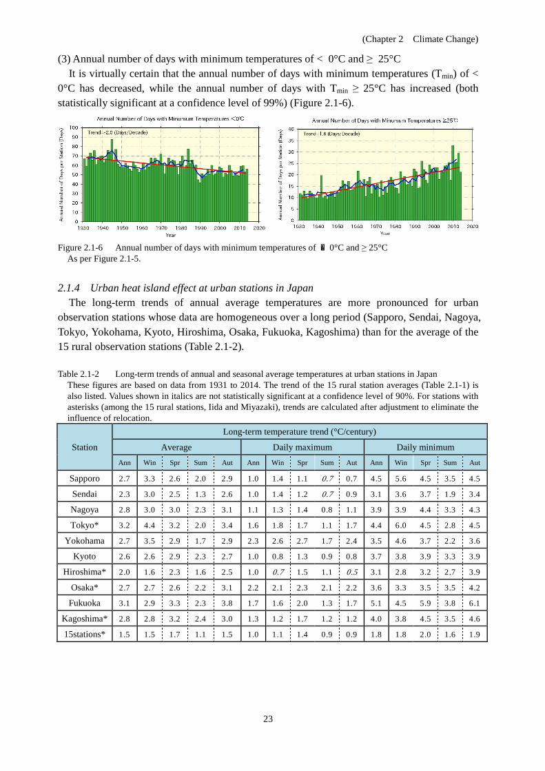
(3) Annual number of days with minimum temperatures of < 0°C and ≥ 25°C It is virtually certain that the annual number of days with minimum temperatures (Tmin) of <
0°C has decreased, while the annual number of days with Tmin ≥ 25°C has increased (both statistically significant at a confidence level of 99%) (Figure 2.1-6).
Figure 2.1-6 Annual number of days with minimum temperatures of <0°C and ≥ 25°C
As per Figure 2.1-5.
2.1.4 Urban heat island effect at urban stations in Japan The long-term trends of annual average temperatures are more pronounced for urban
observation stations whose data are homogeneous over a long period (Sapporo, Sendai, Nagoya, Tokyo, Yokohama, Kyoto, Hiroshima, Osaka, Fukuoka, Kagoshima) than for the average of the 15 rural observation stations (Table 2.1-2). Table 2.1-2 Long-term trends of annual and seasonal average temperatures at urban stations in Japan
These figures are based on data from 1931 to 2014. The trend of the 15 rural station averages (Table 2.1-1) is also listed. Values shown in italics are not statistically significant at a confidence level of 90%. For stations with asterisks (among the 15 rural stations, Iida and Miyazaki), trends are calculated after adjustment to eliminate the influence of relocation.
Station
Long-term temperature trend (°C/century)
Average Daily maximum Daily minimum Ann Win Spr Sum Aut Ann Win Spr Sum Aut Ann Win Spr Sum Aut
Sapporo 2.7 3.3 2.6 2.0 2.9 1.0 1.4 1.1 0.7 0.7 4.5 5.6 4.5 3.5 4.5
Sendai 2.3 3.0 2.5 1.3 2.6 1.0 1.4 1.2 0.7 0.9 3.1 3.6 3.7 1.9 3.4
Nagoya 2.8 3.0 3.0 2.3 3.1 1.1 1.3 1.4 0.8 1.1 3.9 3.9 4.4 3.3 4.3
Tokyo* 3.2 4.4 3.2 2.0 3.4 1.6 1.8 1.7 1.1 1.7 4.4 6.0 4.5 2.8 4.5
Yokohama 2.7 3.5 2.9 1.7 2.9 2.3 2.6 2.7 1.7 2.4 3.5 4.6 3.7 2.2 3.6
Kyoto 2.6 2.6 2.9 2.3 2.7 1.0 0.8 1.3 0.9 0.8 3.7 3.8 3.9 3.3 3.9
Hiroshima* 2.0 1.6 2.3 1.6 2.5 1.0 0.7 1.5 1.1 0.5 3.1 2.8 3.2 2.7 3.9
Osaka* 2.7 2.7 2.6 2.2 3.1 2.2 2.1 2.3 2.1 2.2 3.6 3.3 3.5 3.5 4.2
Fukuoka 3.1 2.9 3.3 2.3 3.8 1.7 1.6 2.0 1.3 1.7 5.1 4.5 5.9 3.8 6.1
Kagoshima* 2.8 2.8 3.2 2.4 3.0 1.3 1.2 1.7 1.2 1.2 4.0 3.8 4.5 3.5 4.6
15stations* 1.5 1.5 1.7 1.1 1.5 1.0 1.1 1.4 0.9 0.9 1.8 1.8 2.0 1.6 1.9
(Chapter 2 Climate Change)
24
As it can be assumed that the long-term trends averaged over the 15 rural stations reflect large-scale climate change, the differences in the long-term trends of urban stations from the average of the 15 stations largely represent the influence of urbanization.
Detailed observation reveals that the long-term trends are more significant in winter, spring and autumn than in summer and more pronounced for minimum temperatures than for maximum temperatures at every urban observation station.
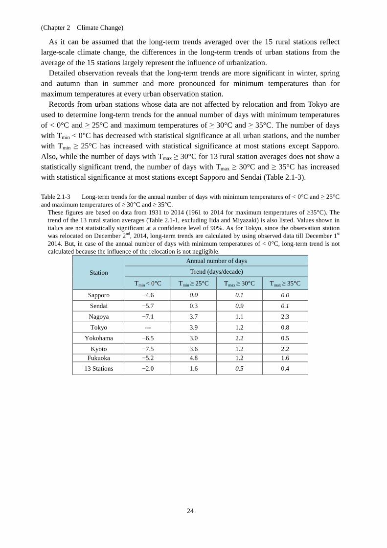
Records from urban stations whose data are not affected by relocation and from Tokyo are used to determine long-term trends for the annual number of days with minimum temperatures of < 0°C and ≥ 25°C and maximum temperatures of ≥ 30°C and ≥ 35°C. The number of days with Tmin < 0°C has decreased with statistical significance at all urban stations, and the number with Tmin ≥ 25°C has increased with statistical significance at most stations except Sapporo. Also, while the number of days with Tmax ≥ 30°C for 13 rural station averages does not show a statistically significant trend, the number of days with Tmax ≥ 30°C and ≥ 35°C has increased with statistical significance at most stations except Sapporo and Sendai (Table 2.1-3). Table 2.1-3 Long-term trends for the annual number of days with minimum temperatures of < 0°C and ≥ 25°C and maximum temperatures of ≥ 30°C and ≥ 35°C.
These figures are based on data from 1931 to 2014 (1961 to 2014 for maximum temperatures of ≥35°C). The trend of the 13 rural station averages (Table 2.1-1, excluding Iida and Miyazaki) is also listed. Values shown in italics are not statistically significant at a confidence level of 90%. As for Tokyo, since the observation station was relocated on December 2nd, 2014, long-term trends are calculated by using observed data till December 1st 2014. But, in case of the annual number of days with minimum temperatures of < 0°C, long-term trend is not calculated because the influence of the relocation is not negligible.
Station
Annual number of days
Trend (days/decade)
Tmin < 0°C Tmin ≥ 25°C Tmax ≥ 30°C Tmax ≥ 35°C
Sapporo −4.6 0.0 0.1 0.0
Sendai −5.7 0.3 0.9 0.1 Nagoya −7.1 3.7 1.1 2.3
Tokyo --- 3.9 1.2 0.8
Yokohama −6.5 3.0 2.2 0.5
Kyoto −7.5 3.6 1.2 2.2 Fukuoka −5.2 4.8 1.2 1.6
13 Stations −2.0 1.6 0.5 0.4

(Chapter 2 Climate Change)
25
2.2 Changes in precipitation13
○ The annual anomaly of global precipitation (for land areas only) in 2014 was 0 mm. ○ The annual anomaly of precipitation in 2014 was +124 mm in Japan. ○ It is virtually certain that the annual numbers of days with precipitation of ≥ 100 mm and ≥ 200 mm are have increased and that the annual number of days with precipitation of ≥ 1.0 mm has decreased.
2.2.1 Global precipitation over land
Annual precipitation (for land areas only) in 2014 was 0 mm above the 1981 – 2010 average (Figure 2.2-1), and the figure has fluctuated periodically since 1901. In the Northern Hemisphere, records show large amounts of rainfall around 1930 and in the 1950s. Long-term trends are not analyzed because the necessary precipitation data for sea areas are not available.
Figure 2.2-1 Annual anomalies in precipitation (over land areas only) from 1901 to 2014 for the globe (top left), for the Northern Hemisphere (top right) and for the Southern Hemisphere (bottom). Anomalies are deviations from the baseline (the 1981 – 2010 average).
The bars indicate the precipitation anomaly for each year, and the blue line indicates the five-year running mean.
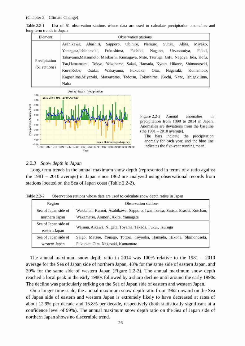
2.2.2 Precipitation over Japan
This section describes long-term trends in precipitation over Japan as derived from analysis of precipitation records from 51 observation stations (Table 2.2-1).
Annual precipitation in 2014 was +123.8 mm above the 1981 – 2010 average. Japan experienced relatively large amounts of rainfall until the mid-1920s and around the 1950s. The annual figure has become more variable since the 1970s (Figure 2.2-2).
13 Data on annual precipitation around the world and in Japan are published on JMA’s website.
http://www.data.jma.go.jp/cpdinfo/temp/index.html (Japanese) http://ds.data.jma.go.jp/tcc/tcc/products/gwp/gwp.html (English)
(Chapter 2 Climate Change)
26
Table 2.2-1 List of 51 observation stations whose data are used to calculate precipitation anomalies and long-term trends in Japan
Element Observation stations
Precipitation (51 stations)
Asahikawa, Abashiri, Sapporo, Obihiro, Nemuro, Suttsu, Akita, Miyako, Yamagata,Ishinomaki, Fukushima, Fushiki, Nagano, Utsunomiya, Fukui, Takayama,Matsumoto, Maebashi, Kumagaya, Mito, Tsuruga, Gifu, Nagoya, Iida, Kofu, Tsu,Hamamatsu, Tokyo, Yokohama, Sakai, Hamada, Kyoto, Hikone, Shimonoseki, Kure,Kobe, Osaka, Wakayama, Fukuoka, Oita, Nagasaki, Kumamoto, Kagoshima,Miyazaki, Matsuyama, Tadotsu, Tokushima, Kochi, Naze, Ishigakijima, Naha
Figure 2.2-2 Annual anomalies in precipitation from 1898 to 2014 in Japan. Anomalies are deviations from the baseline (the 1981 – 2010 average).
The bars indicate the precipitation anomaly for each year, and the blue line indicates the five-year running mean.
2.2.3 Snow depth in Japan Long-term trends in the annual maximum snow depth (represented in terms of a ratio against
the 1981 – 2010 average) in Japan since 1962 are analyzed using observational records from stations located on the Sea of Japan coast (Table 2.2-2).
Table 2.2-2 Observation stations whose data are used to calculate snow depth ratios in Japan
Region Observation stations
Sea of Japan side of northern Japan
Wakkanai, Rumoi, Asahikawa, Sapporo, Iwamizawa, Suttsu, Esashi, Kutchan, Wakamatsu, Aomori, Akita, Yamagata
Sea of Japan side of eastern Japan
Wajima, Aikawa, Niigata, Toyama, Takada, Fukui, Tsuruga
Sea of Japan side of western Japan
Saigo, Matsue, Yonago, Tottori, Toyooka, Hamada, Hikone, Shimonoseki, Fukuoka, Oita, Nagasaki, Kumamoto
The annual maximum snow depth ratio in 2014 was 100% relative to the 1981 – 2010 average for the Sea of Japan side of northern Japan, 48% for the same side of eastern Japan, and 39% for the same side of western Japan (Figure 2.2-3). The annual maximum snow depth reached a local peak in the early 1980s followed by a sharp decline until around the early 1990s. The decline was particularly striking on the Sea of Japan side of eastern and western Japan.
On a longer time scale, the annual maximum snow depth ratio from 1962 onward on the Sea of Japan side of eastern and western Japan is extremely likely to have decreased at rates of about 12.9% per decade and 15.8% per decade, respectively (both statistically significant at a confidence level of 99%). The annual maximum snow depth ratio on the Sea of Japan side of northern Japan shows no discernible trend.

(Chapter 2 Climate Change)
27
Figure 2.2-3 Annual maximum snow depth ratio from 1962 to 2014 on the Sea of Japan side for northern Japan (top left), eastern Japan (top right) and western Japan (bottom). Annual averages are presented as ratios against the baseline (the 1981 – 2010 average).
The bars indicate the snow depth ratio for each year. The blue line indicates the five-year running mean, and the red line indicates the long-term linear trend.
2.2.4 Long-term trends of extreme precipitation events in Japan This section describes long-term trends in frequencies of extremely wet/dry months and
heavy daily precipitation events in Japan based on analysis of precipitation data from 51 observation stations. (1) Extremely wet/dry months14
It is virtually certain that the frequency of extremely dry months increased during the period from 1901 to 2014 (statistically significant at a confidence level of 99%) (Figure2.2-4 left). There has been no discernible trend in the frequency of extremely wet months (Figure2.2-4 right).
Figure 2.2-4 Annual number of extremely wet/dry months The graphs show the annual number of occurrences of the first-to-forth heaviest/lightest precipitation values for each month during the period from 1901 to 2014. The green bars indicate annual occurrences of extremely heavy/light monthly precipitation divided by the total number of monthly observation data sets available for the year (i.e., the average occurrence per station). The blue line indicates the five-year running mean, and the straight red line indicates the long-term liner trend.
14 Here, judgment of extremely heavy/light precipitation is based on the fourth–highest/lowest monthly values on record over the 114-year period from 1901 to 2014. The frequency of occurrence of the highest/lowest to the fourth–highest/lowest values over the this period is approximately once every 29 years, which is close to JMA’s definition of extreme climate events as those occurring once every 30 years or longer (See the Glossary for terms relating to Extreme climate event).

(Chapter 2 Climate Change)
28
(2) Annual number of days with precipitation of ≥ 100 mm, ≥ 200 mm and ≥ 1.0 mm It is virtually certain that the annual numbers of days with precipitation of ≥ 100 mm and ≥ 200 mm (Figure 2.2-5) have increased from 1901 to 2014 and that the annual number of days with precipitation of ≥ 1.0 mm (Figure 2.2-6) has decreased over the same period (statistically significant at a confidence level of 99%). These results suggest decrease in the annual number of wet days including light precipitation and in contrast, an increase in extremely wet days.
Figure 2.2-5 Annual number of days with precipitation ≥ 100 mm and ≥ 200 mm The blue line indicates the five-year running mean, and the straight red line indicates the long-term liner trend.
Figure 2.2-6 Annual number of days with precipitation of ≥ 1.0 mm
As per figure 2.2-5.
2.2.5 Long-term trends of heavy rainfall analyzed using AMeDAS data
JMA operationally observes precipitation at about 1,300 unmanned regional meteorological observation stations all over Japan (collectively known as the Automated Meteorological Data Acquisition System, or AMeDAS). Observation was started in the latter part of the 1970s at many points, and observation data covering the 39-year period through to 2014 are available. Although the period covered by AMeDAS observation records is shorter than that of Local Meteorological Observatories or Weather Stations (which have observation records for the past 100 years or so), there are around eight times as many AMeDAS stations as Local Meteorological Observatories and Weather Stations combined. Hence, AMeDAS is better equipped to capture heavy precipitation events that take place on a limited spatial scale.
Here, trends in annual number of events with extreme precipitation exceeding 50 mm/80 mm per hour (every-hour-on-the-hour observations) (Figure 2.2-7) and 200 mm/400 mm per day (Figure 2.2-8) are described based on AMeDAS observation data15. 15 The number of AMeDAS station was about 800 in 1976, and had gradually increased to about 1,300 by 2014. To account for these numerical differences, the annual number of precipitation events needs to be converted to a per-1,000-station basis. Data from wireless robot precipitation observation stations previously deployed in mountainous areas are also excluded.
(Chapter 2 Climate Change)
29
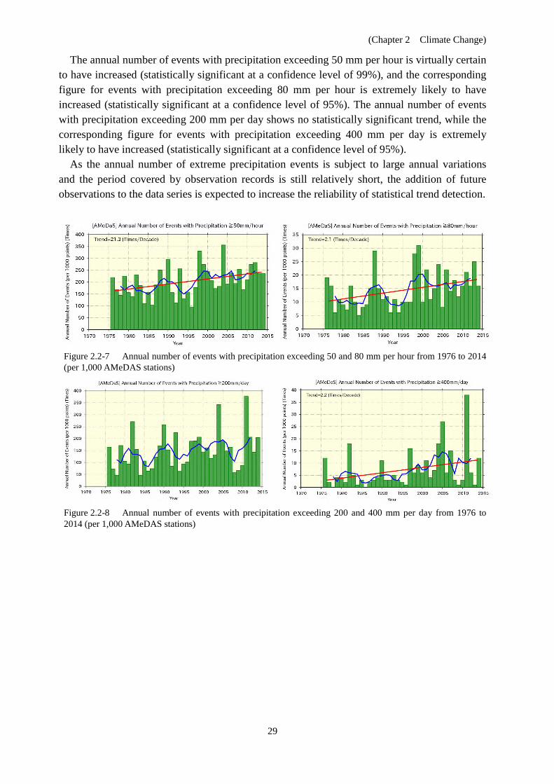
The annual number of events with precipitation exceeding 50 mm per hour is virtually certain to have increased (statistically significant at a confidence level of 99%), and the corresponding figure for events with precipitation exceeding 80 mm per hour is extremely likely to have increased (statistically significant at a confidence level of 95%). The annual number of events with precipitation exceeding 200 mm per day shows no statistically significant trend, while the corresponding figure for events with precipitation exceeding 400 mm per day is extremely likely to have increased (statistically significant at a confidence level of 95%).
As the annual number of extreme precipitation events is subject to large annual variations and the period covered by observation records is still relatively short, the addition of future observations to the data series is expected to increase the reliability of statistical trend detection.
Figure 2.2-7 Annual number of events with precipitation exceeding 50 and 80 mm per hour from 1976 to 2014 (per 1,000 AMeDAS stations)
Figure 2.2-8 Annual number of events with precipitation exceeding 200 and 400 mm per day from 1976 to 2014 (per 1,000 AMeDAS stations)
(Chapter 2 Climate Change)
30
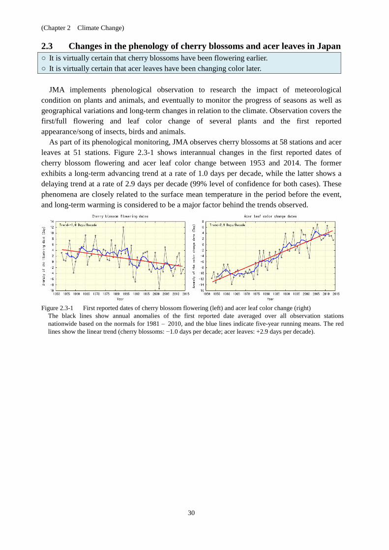
2.3 Changes in the phenology of cherry blossoms and acer leaves in Japan ○ It is virtually certain that cherry blossoms have been flowering earlier. ○ It is virtually certain that acer leaves have been changing color later.
JMA implements phenological observation to research the impact of meteorological
condition on plants and animals, and eventually to monitor the progress of seasons as well as geographical variations and long-term changes in relation to the climate. Observation covers the first/full flowering and leaf color change of several plants and the first reported appearance/song of insects, birds and animals.
As part of its phenological monitoring, JMA observes cherry blossoms at 58 stations and acer leaves at 51 stations. Figure 2.3-1 shows interannual changes in the first reported dates of cherry blossom flowering and acer leaf color change between 1953 and 2014. The former exhibits a long-term advancing trend at a rate of 1.0 days per decade, while the latter shows a delaying trend at a rate of 2.9 days per decade (99% level of confidence for both cases). These phenomena are closely related to the surface mean temperature in the period before the event, and long-term warming is considered to be a major factor behind the trends observed.
Figure 2.3-1 First reported dates of cherry blossom flowering (left) and acer leaf color change (right)
The black lines show annual anomalies of the first reported date averaged over all observation stations nationwide based on the normals for 1981 – 2010, and the blue lines indicate five-year running means. The red lines show the linear trend (cherry blossoms: −1.0 days per decade; acer leaves: +2.9 days per decade).
(Chapter 2 Climate Change)
31
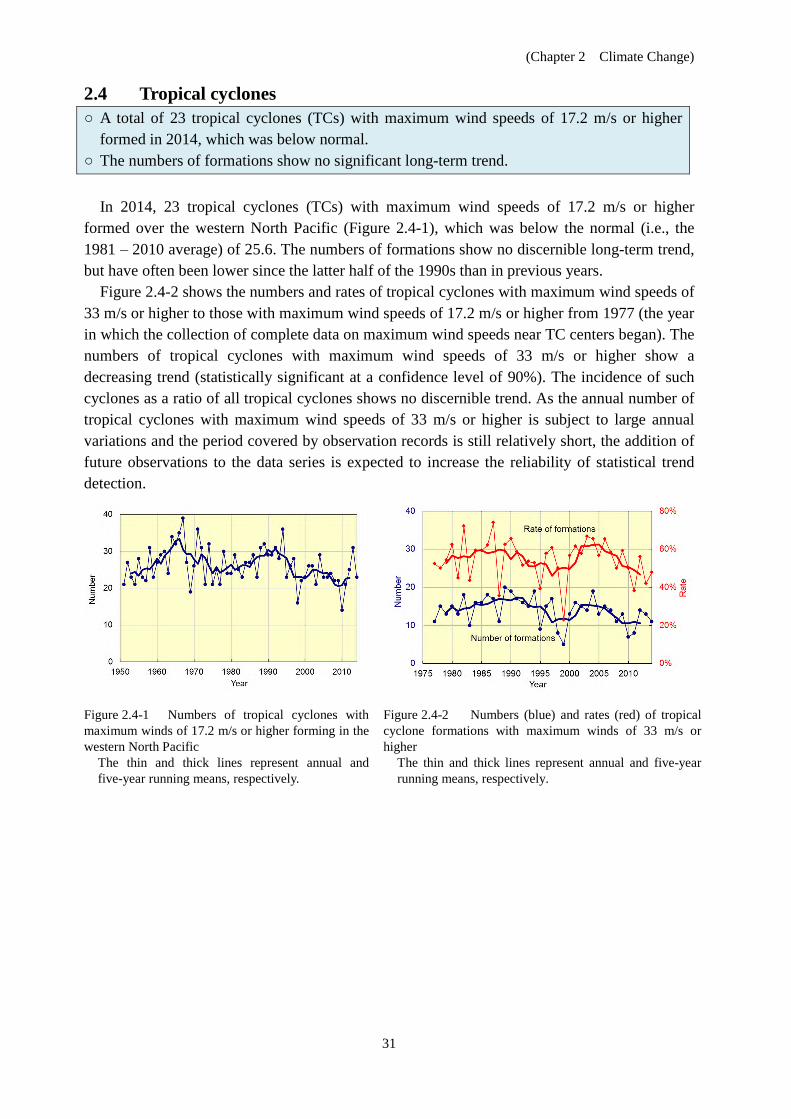
2.4 Tropical cyclones ○ A total of 23 tropical cyclones (TCs) with maximum wind speeds of 17.2 m/s or higher
formed in 2014, which was below normal. ○ The numbers of formations show no significant long-term trend.
In 2014, 23 tropical cyclones (TCs) with maximum wind speeds of 17.2 m/s or higher
formed over the western North Pacific (Figure 2.4-1), which was below the normal (i.e., the 1981 – 2010 average) of 25.6. The numbers of formations show no discernible long-term trend, but have often been lower since the latter half of the 1990s than in previous years.
Figure 2.4-2 shows the numbers and rates of tropical cyclones with maximum wind speeds of 33 m/s or higher to those with maximum wind speeds of 17.2 m/s or higher from 1977 (the year in which the collection of complete data on maximum wind speeds near TC centers began). The numbers of tropical cyclones with maximum wind speeds of 33 m/s or higher show a decreasing trend (statistically significant at a confidence level of 90%). The incidence of such cyclones as a ratio of all tropical cyclones shows no discernible trend. As the annual number of tropical cyclones with maximum wind speeds of 33 m/s or higher is subject to large annual variations and the period covered by observation records is still relatively short, the addition of future observations to the data series is expected to increase the reliability of statistical trend detection.
Figure 2.4-1 Numbers of tropical cyclones with maximum winds of 17.2 m/s or higher forming in the western North Pacific
The thin and thick lines represent annual and five-year running means, respectively.
Figure 2.4-2 Numbers (blue) and rates (red) of tropical cyclone formations with maximum winds of 33 m/s or higher
The thin and thick lines represent annual and five-year running means, respectively.

(Chapter 2 Climate Change)
32
2.5 Sea surface temperature16 ○ The annual mean global average sea surface temperature (SST) in 2014 was 0.20°C above
the 1981 – 2010 average, which was the highest since 1891. ○ The global average SST has risen at a rate of about 0.51°C per century. ○ Annual average SSTs around Japan have risen by +1.07°C per century. 2.5.1 Global sea surface temperature
The annual mean global average SST in 2014 was 0.20°C above the 1981 – 2010 average. This was much higher than the previous highest value of 0.14°C observed in 1998, and was the highest since 1891. The linear trend from 1891 to 2014 shows an increase of 0.51°C per century (Figure 2.5-1). The linear trend of the average SST for each ocean basin varies from +0.43 to +0.71°C per century (Figure 2.5-2). The warming trends for the global average and each ocean basin are statistically significant at a confidence level of 99%.
The global average SST has long been rising with repeated upward and downward variations as with the global average surface temperature (see Section 2.1), which is used as a global warming metric. On a multi-year time scale, the global average SST showed a warming trend from the middle of the 1970s to around 2000 and has remained at the same level for the last decade (see the blue line in Figure 2.5-1). This is partly because internal decadal to multi-decadal variations in the climate system overlap with the rising trends. It is important to estimate the contribution of these internal variations in order to properly understand global warming. In the next section, Pacific Decadal Oscillation (PDO) is presented as a typical example of decadal variability observed in SSTs.
Figure 2.5-1 Long-term change in annual anomalies of the global average sea surface temperature from 1891 to 2014
The thin black line indicates anomalies of the global sea surface temperature in each year. The blue line indicates five-year running mean, and the red line indicates a long-term linear trend. Anomalies are deviations from the 1981 – 2010 average.
Figure 2.5-2 Rates of mean rise for each ocean (°C per century)
Rates covering the period from 1891 to 2014 are shown (The warming trends are all statistically significant at a confidence level of 99%).
16 The results of analysis regarding tendencies of SSTs worldwide and around Japan are published on JMA’s website. http://www.data.jma.go.jp/gmd/kaiyou/english/long_term_sst_global/glb_warm_e.html http://www.data.jma.go.jp/gmd/kaiyou/english/long_term_sst_japan/sea_surface_temperature_around_japan.html
(Chapter 2 Climate Change)
33
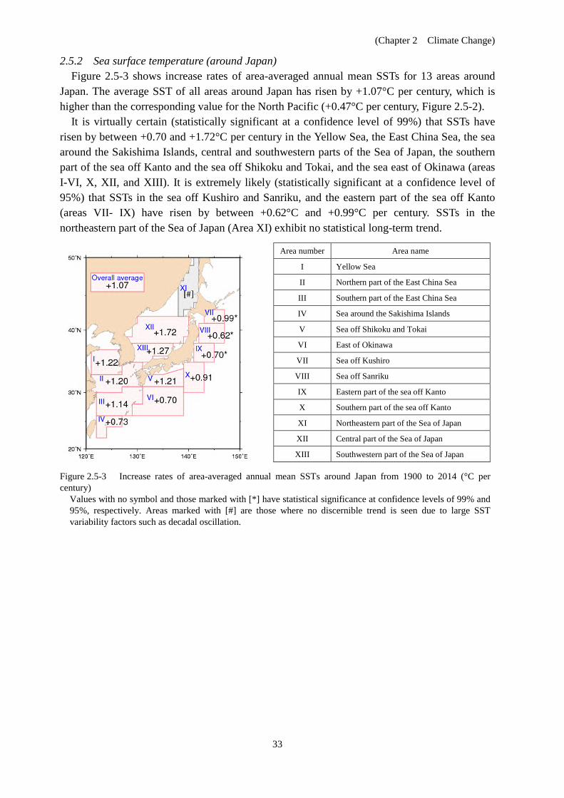
2.5.2 Sea surface temperature (around Japan) Figure 2.5-3 shows increase rates of area-averaged annual mean SSTs for 13 areas around
Japan. The average SST of all areas around Japan has risen by +1.07°C per century, which is higher than the corresponding value for the North Pacific (+0.47°C per century, Figure 2.5-2).
It is virtually certain (statistically significant at a confidence level of 99%) that SSTs have risen by between +0.70 and +1.72°C per century in the Yellow Sea, the East China Sea, the sea around the Sakishima Islands, central and southwestern parts of the Sea of Japan, the southern part of the sea off Kanto and the sea off Shikoku and Tokai, and the sea east of Okinawa (areas I-VI, X, XII, and XIII). It is extremely likely (statistically significant at a confidence level of 95%) that SSTs in the sea off Kushiro and Sanriku, and the eastern part of the sea off Kanto (areas VII- IX) have risen by between +0.62°C and +0.99°C per century. SSTs in the northeastern part of the Sea of Japan (Area XI) exhibit no statistical long-term trend.
Area number Area name
I Yellow Sea
II Northern part of the East China Sea
III Southern part of the East China Sea
IV Sea around the Sakishima Islands
V Sea off Shikoku and Tokai
VI East of Okinawa
VII Sea off Kushiro
VIII Sea off Sanriku
IX Eastern part of the sea off Kanto
X Southern part of the sea off Kanto
XI Northeastern part of the Sea of Japan
XII Central part of the Sea of Japan
XIII Southwestern part of the Sea of Japan
Figure 2.5-3 Increase rates of area-averaged annual mean SSTs around Japan from 1900 to 2014 (°C per century)
Values with no symbol and those marked with [*] have statistical significance at confidence levels of 99% and 95%, respectively. Areas marked with [#] are those where no discernible trend is seen due to large SST variability factors such as decadal oscillation.
(Chapter 2 Climate Change)
34
2.6 El Niño/La Niña 17 and PDO (Pacific Decadal Oscillation) 18 ○ An El Niño event emerged in summer 2014 and continued for the rest of the year. ○ Although negative PDO index values have generally been observed since around 2000, the
annual mean value turned positive in 2014. 2.6.1 El Niño/La Niña
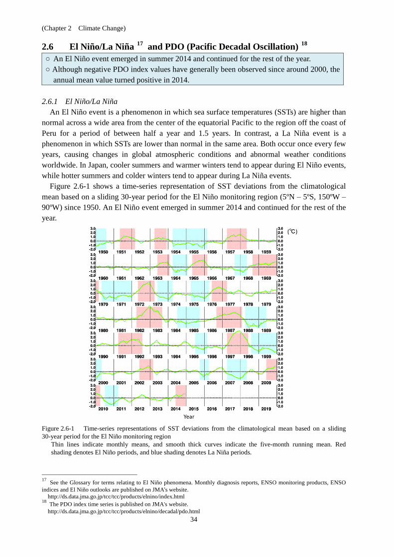
An El Niño event is a phenomenon in which sea surface temperatures (SSTs) are higher than normal across a wide area from the center of the equatorial Pacific to the region off the coast of Peru for a period of between half a year and 1.5 years. In contrast, a La Niña event is a phenomenon in which SSTs are lower than normal in the same area. Both occur once every few years, causing changes in global atmospheric conditions and abnormal weather conditions worldwide. In Japan, cooler summers and warmer winters tend to appear during El Niño events, while hotter summers and colder winters tend to appear during La Niña events.
Figure 2.6-1 shows a time-series representation of SST deviations from the climatological mean based on a sliding 30-year period for the El Niño monitoring region (5ºN – 5ºS, 150ºW – 90ºW) since 1950. An El Niño event emerged in summer 2014 and continued for the rest of the year.
Figure 2.6-1 Time-series representations of SST deviations from the climatological mean based on a sliding 30-year period for the El Niño monitoring region
Thin lines indicate monthly means, and smooth thick curves indicate the five-month running mean. Red shading denotes El Niño periods, and blue shading denotes La Niña periods.
17 See the Glossary for terms relating to El Niño phenomena. Monthly diagnosis reports, ENSO monitoring products, ENSO indices and El Niño outlooks are published on JMA’s website.
http://ds.data.jma.go.jp/tcc/tcc/products/elnino/index.html 18 The PDO index time series is published on JMA's website.
http://ds.data.jma.go.jp/tcc/tcc/products/elnino/decadal/pdo.html
(Chapter 2 Climate Change)
35
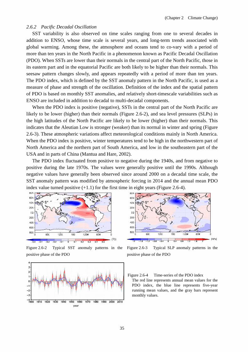
2.6.2 Pacific Decadal Oscillation SST variability is also observed on time scales ranging from one to several decades in
addition to ENSO, whose time scale is several years, and long-term trends associated with global warming. Among these, the atmosphere and oceans tend to co-vary with a period of more than ten years in the North Pacific in a phenomenon known as Pacific Decadal Oscillation (PDO). When SSTs are lower than their normals in the central part of the North Pacific, those in its eastern part and in the equatorial Pacific are both likely to be higher than their normals. This seesaw pattern changes slowly, and appears repeatedly with a period of more than ten years. The PDO index, which is defined by the SST anomaly pattern in the North Pacific, is used as a measure of phase and strength of the oscillation. Definition of the index and the spatial pattern of PDO is based on monthly SST anomalies, and relatively short-timescale variabilities such as ENSO are included in addition to decadal to multi-decadal components.
When the PDO index is positive (negative), SSTs in the central part of the North Pacific are likely to be lower (higher) than their normals (Figure 2.6-2), and sea level pressures (SLPs) in the high latitudes of the North Pacific are likely to be lower (higher) than their normals. This indicates that the Aleutian Low is stronger (weaker) than its normal in winter and spring (Figure 2.6-3). These atmospheric variations affect meteorological conditions mainly in North America. When the PDO index is positive, winter temperatures tend to be high in the northwestern part of North America and the northern part of South America, and low in the southeastern part of the USA and in parts of China (Mantua and Hare, 2002).
The PDO index fluctuated from positive to negative during the 1940s, and from negative to positive during the late 1970s. The values were generally positive until the 1990s. Although negative values have generally been observed since around 2000 on a decadal time scale, the SST anomaly pattern was modified by atmospheric forcing in 2014 and the annual mean PDO index value turned positive (+1.1) for the first time in eight years (Figure 2.6-4).
Figure 2.6-2 Typical SST anomaly patterns in the positive phase of the PDO
Figure 2.6-3 Typical SLP anomaly patterns in the positive phase of the PDO
Figure 2.6-4 Time-series of the PDO index
The red line represents annual mean values for the PDO index, the blue line represents five-year running mean values, and the gray bars represent monthly values.

(Chapter 2 Climate Change)
36
2.7 Global upper ocean heat content19 ○ An increase in globally integrated upper ocean heat content was observed from 1950 to
2014 with a linear trend of 2.11 × 10²² J per decade. Oceans have a significant impact on the global climate because they cover about 70% of the
earth’s surface and have high heat capacity. According to the Intergovernmental Panel on Climate Change Fifth Assessment report (IPCC, 2013), more than 60% of the net energy increase in the climate system from 1971 to 2010 is stored in the upper ocean (0 – 700 m), and about 30% is stored below 700 m. Oceanic warming results in sea level rises due to thermal expansion.
It is virtually certain that globally integrated upper ocean (0 – 700 m) heat content (OHC) rose between 1950 and 2014 at a rate of 2.11 × 10²² J per decade as a long-term trend with interannual variations (statistically significant at a confidence level of 99%) (Figure 2.7-1). OHC exhibited marked increases from the mid-1990s to the early 2000s and slight increases for the next several years, as seen with the global mean surface temperature and the sea surface temperature. Since the mid-2000s OHC has increased again significantly. A rise of 0.022°C per decade in the globally averaged upper ocean (0 – 700 m) temperature has accompanied the OHC increase. These long-term trends can be attributed to global warming caused by increased concentrations of anthropogenic greenhouse gases such as CO2 as well as natural variability.
19 The results of ocean heat content analysis are published on JMA’s website.
http://www.data.jma.go.jp/gmd/kaiyou/english/ohc/ohc_global_en.html
Figure 2.7-1 Time-series representation of the globally integrated upper ocean (0 – 700 m) heat content anomaly
The 1981 – 2010 average is referenced as the normal.
(Chapter 2 Climate Change)
37
2.8 Sea levels around Japan 20 ○ A trend of sea level rise has been seen in Japanese coastal areas since the 1980s. ○ No clear trend of sea level rise was seen in Japanese coastal areas for the period from 1906
to 2014. The IPCC Fifth Assessment report (2013) concluded that the global mean sea level had risen
due mainly to 1) oceanic thermal expansion, 2) changes in mountain glaciers, the Greenland ice sheet and the Antarctic ice sheet, and 3) changes in land water storage. The report also said it is very likely that the mean rate of global average sea level rise was 1.7 [1.5 to 1.9] mm/year between 1901 and 2010, 2.0 [1.7 to 2.3] mm/year between 1971 and 2010, and 3.2 [2.8 to 3.6] mm/year between 1993 and 2010. (The values in square brackets show the 90% uncertainty range.)
A trend of sea level rise has been seen in Japanese coastal areas since the 1980s. The rate of rise around the country was 1.1 [0.6 to 1.6] mm/year from 1971 to 2010 and 2.8 [1.3 to 4.3] mm/year from 1993 to 2010. These figures are comparable to those observed for the global average in recent years. In contrast, sea levels in Japanese coastal areas showed no significant rise from 1906 to 2010, as shown in Figure 2.8-1. One reason for this difference is that “shifting surface winds, the expansion of warming ocean water, and the addition of melting ice can alter ocean currents which, in turn, lead to changes in sea level that vary from place to place” (IPCC, 2013). However, as the full range of reasons for the difference has not yet been elucidated, further research in this area is needed.
Variations with 10- to 20-year periods (near-10-year variations) are seen for the period from 1906 to 2014, with the maximum sea level appearing around 1950. Analysis has shown that the near-10-year variations observed are caused by changes in the strength and meridional movement of westerlies over the North Pacific. By way of example, anticyclonic wind anomalies over the North Pacific cause sea level rise in the central North Pacific. The positive sea level anomaly propagates westward due to the effect of the earth’s rotation, causing sea level rise around Japan.
20 Sea levels around Japan are published on the JMA’s website.
http://www.data.jma.go.jp/gmd/kaiyou/english/sl_trend/sea_level_around_japan.html
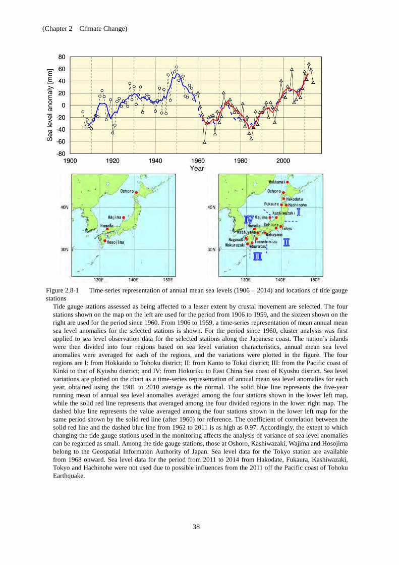
(Chapter 2 Climate Change)
38
Figure 2.8-1 Time-series representation of annual mean sea levels (1906 – 2014) and locations of tide gauge stations
Tide gauge stations assessed as being affected to a lesser extent by crustal movement are selected. The four stations shown on the map on the left are used for the period from 1906 to 1959, and the sixteen shown on the right are used for the period since 1960. From 1906 to 1959, a time-series representation of mean annual mean sea level anomalies for the selected stations is shown. For the period since 1960, cluster analysis was first applied to sea level observation data for the selected stations along the Japanese coast. The nation’s islands were then divided into four regions based on sea level variation characteristics, annual mean sea level anomalies were averaged for each of the regions, and the variations were plotted in the figure. The four regions are I: from Hokkaido to Tohoku district; II: from Kanto to Tokai district; III: from the Pacific coast of Kinki to that of Kyushu district; and IV: from Hokuriku to East China Sea coast of Kyushu district. Sea level variations are plotted on the chart as a time-series representation of annual mean sea level anomalies for each year, obtained using the 1981 to 2010 average as the normal. The solid blue line represents the five-year running mean of annual sea level anomalies averaged among the four stations shown in the lower left map, while the solid red line represents that averaged among the four divided regions in the lower right map. The dashed blue line represents the value averaged among the four stations shown in the lower left map for the same period shown by the solid red line (after 1960) for reference. The coefficient of correlation between the solid red line and the dashed blue line from 1962 to 2011 is as high as 0.97. Accordingly, the extent to which changing the tide gauge stations used in the monitoring affects the analysis of variance of sea level anomalies can be regarded as small. Among the tide gauge stations, those at Oshoro, Kashiwazaki, Wajima and Hosojima belong to the Geospatial Informaton Authority of Japan. Sea level data for the Tokyo station are available from 1968 onward. Sea level data for the period from 2011 to 2014 from Hakodate, Fukaura, Kashiwazaki, Tokyo and Hachinohe were not used due to possible influences from the 2011 off the Pacific coast of Tohoku Earthquake.
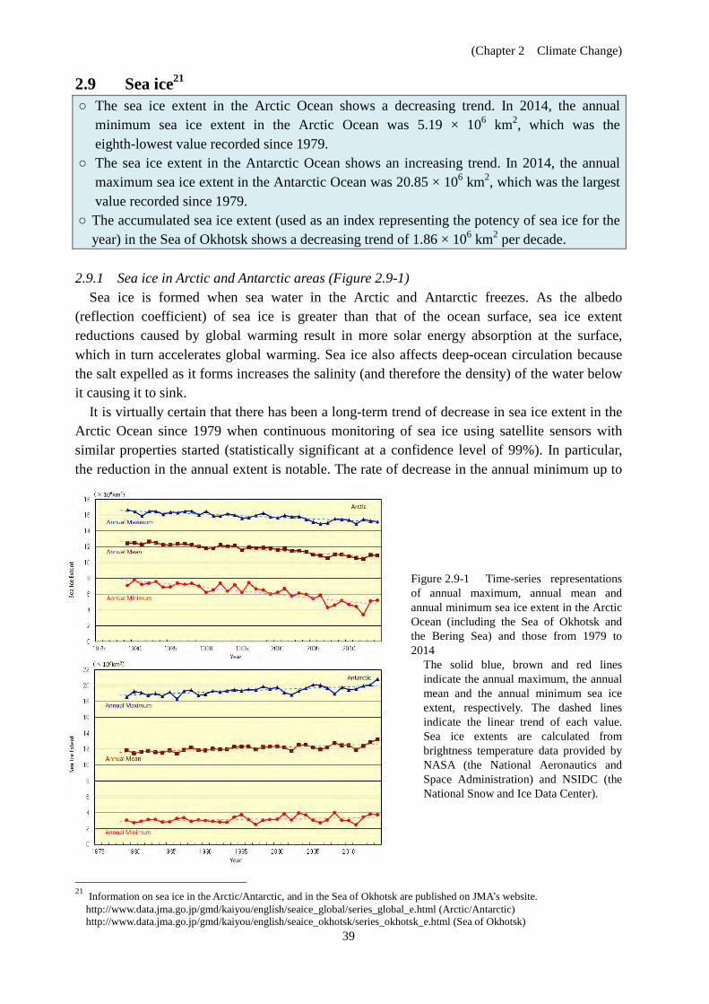
(Chapter 2 Climate Change)
39
2.9 Sea ice21 ○ The sea ice extent in the Arctic Ocean shows a decreasing trend. In 2014, the annual
minimum sea ice extent in the Arctic Ocean was 5.19 × 10⁶ km2, which was the eighth-lowest value recorded since 1979.
○ The sea ice extent in the Antarctic Ocean shows an increasing trend. In 2014, the annual maximum sea ice extent in the Antarctic Ocean was 20.85 × 10⁶ km2, which was the largest value recorded since 1979.
○ The accumulated sea ice extent (used as an index representing the potency of sea ice for the year) in the Sea of Okhotsk shows a decreasing trend of 1.86 × 10⁶ km2 per decade.
2.9.1 Sea ice in Arctic and Antarctic areas (Figure 2.9-1)
Sea ice is formed when sea water in the Arctic and Antarctic freezes. As the albedo (reflection coefficient) of sea ice is greater than that of the ocean surface, sea ice extent reductions caused by global warming result in more solar energy absorption at the surface, which in turn accelerates global warming. Sea ice also affects deep-ocean circulation because the salt expelled as it forms increases the salinity (and therefore the density) of the water below it causing it to sink.
It is virtually certain that there has been a long-term trend of decrease in sea ice extent in the Arctic Ocean since 1979 when continuous monitoring of sea ice using satellite sensors with similar properties started (statistically significant at a confidence level of 99%). In particular, the reduction in the annual extent is notable. The rate of decrease in the annual minimum up to
21 Information on sea ice in the Arctic/Antarctic, and in the Sea of Okhotsk are published on JMA’s website.
http://www.data.jma.go.jp/gmd/kaiyou/english/seaice_global/series_global_e.html (Arctic/Antarctic) http://www.data.jma.go.jp/gmd/kaiyou/english/seaice_okhotsk/series_okhotsk_e.html (Sea of Okhotsk)
Figure 2.9-1 Time-series representations of annual maximum, annual mean and annual minimum sea ice extent in the Arctic Ocean (including the Sea of Okhotsk and the Bering Sea) and those from 1979 to 2014
The solid blue, brown and red lines indicate the annual maximum, the annual mean and the annual minimum sea ice extent, respectively. The dashed lines indicate the linear trend of each value. Sea ice extents are calculated from brightness temperature data provided by NASA (the National Aeronautics and Space Administration) and NSIDC (the National Snow and Ice Data Center).

(Chapter 2 Climate Change)
40
2014 was 0.089 × 10⁶ km2 per year and the annual minimum was 5.19 × 10⁶ km2, which was the eighth-lowest record since 1979. The annual mean sea ice extent in the Arctic Ocean shows a decreasing trend of 0.057 × 10⁶ km2 per year Meanwhile, it is virtually certain that there has been an increase at a rate of 0.029 × 10⁶ km2 per year in the annual mean sea ice extent in the Antarctic Ocean (statistically significant at the confidence level of 99%). The value for 2014 was 20.85 × 10⁶ km2, which was the largest recorded since 1979. 2.9.2 Sea ice in the Sea of Okhotsk (Figure 2.9-2)
The Sea of Okhotsk is the southernmost sea in the Northern Hemisphere where sea ice is observed across a wide area. The variation of the sea ice in the Sea of Okhotsk has effect on climate in coastal area facing the Sea of Okhotsk in Hokkaido and water quality of Oyashio.
The accumulated22 and maximum23 sea ice extents in the Sea of Okhotsk show large interannual variations. However, it is virtually certain that they exhibited a long-term trend of decrease for the period from 1971 to 2014 (statistically significant at the confidence level of 99%). The accumulated sea ice extent (used as an index showing the potency of sea ice for the year) has decreased by 1.86 × 10⁶ km2 per decade, and the maximum extent has decreased by 0.06 × 10⁶ km2 per decade (corresponding to 3.8% of the Sea of Okhotsk’s total area).
Figure 2.9-2 Time-series representations of maximum sea ice extent (red) and accumulated sea ice extent (blue) for the Sea of Okhotsk from 1971 to 2014
Straight lines indicate the linear trend of each.
2.10 Snow cover in the Northern Hemisphere ○ A decreasing trend is observed in the interannual variability of the total snow cover extent
in the Northern Hemisphere for May, September, November, and December. ○ In winter 2013/2014, there were more days of snow cover than normal in the central to
eastern USA, and fewer days in the western USA. The albedo of snow-covered ground (i.e., the ratio of solar radiation reflected by the surface)
is higher than that of snow-free ground. The variability of snow cover has an impact on the earth’s surface energy budget and radiation balance, and therefore on the climate. In addition, snow absorbs heat from its surroundings and melts, thereby providing soil moisture and related effects on the climate system. The variability of atmospheric circulation and oceanographic conditions affects the amount of snow cover, which exhibits a close and mutual association with climatic conditions. JMA monitors snow-cover variations in the Northern Hemisphere using 22 The accumulated sea ice extent: It shows the seasonal summation of sea ice extent of every five days from December 5 in the previous year to May 31. It is used as the index shows the potency of sea ice in the year. 23 The maximum sea ice extent: It shows sea ice extent that sea ice was the most expanding of every five days in the course of the year.
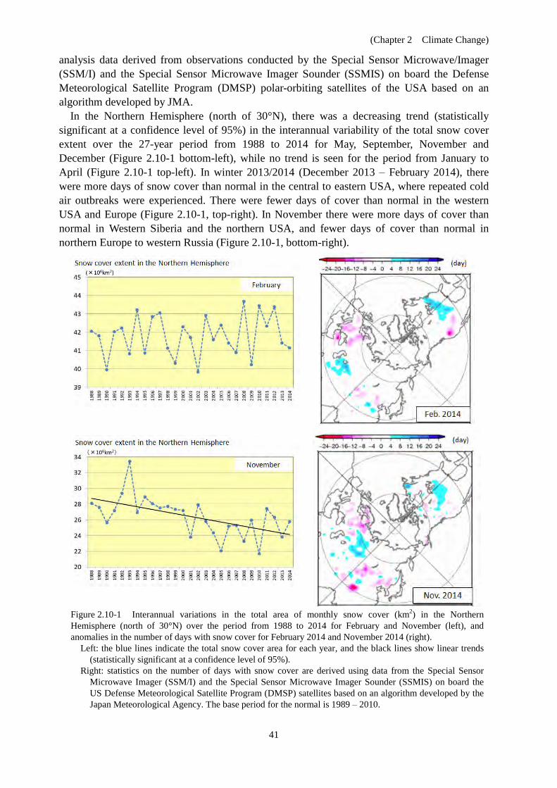
(Chapter 2 Climate Change)
41
analysis data derived from observations conducted by the Special Sensor Microwave/Imager (SSM/I) and the Special Sensor Microwave Imager Sounder (SSMIS) on board the Defense Meteorological Satellite Program (DMSP) polar-orbiting satellites of the USA based on an algorithm developed by JMA.
In the Northern Hemisphere (north of 30°N), there was a decreasing trend (statistically significant at a confidence level of 95%) in the interannual variability of the total snow cover extent over the 27-year period from 1988 to 2014 for May, September, November and December (Figure 2.10-1 bottom-left), while no trend is seen for the period from January to April (Figure 2.10-1 top-left). In winter 2013/2014 (December 2013 – February 2014), there were more days of snow cover than normal in the central to eastern USA, where repeated cold air outbreaks were experienced. There were fewer days of cover than normal in the western USA and Europe (Figure 2.10-1, top-right). In November there were more days of cover than normal in Western Siberia and the northern USA, and fewer days of cover than normal in northern Europe to western Russia (Figure 2.10-1, bottom-right).
Figure 2.10-1 Interannual variations in the total area of monthly snow cover (km2) in the Northern Hemisphere (north of 30°N) over the period from 1988 to 2014 for February and November (left), and anomalies in the number of days with snow cover for February 2014 and November 2014 (right).
Left: the blue lines indicate the total snow cover area for each year, and the black lines show linear trends (statistically significant at a confidence level of 95%).
Right: statistics on the number of days with snow cover are derived using data from the Special Sensor Microwave Imager (SSM/I) and the Special Sensor Microwave Imager Sounder (SSMIS) on board the US Defense Meteorological Satellite Program (DMSP) satellites based on an algorithm developed by the Japan Meteorological Agency. The base period for the normal is 1989 – 2010.

(Chapter 3 Atmospheric and Marine Environment Monitoring)
42
Chapter 3 Atmospheric and Marine Environment Monitoring
3.1 Monitoring of greenhouse gases24 ○ The global concentration of carbon dioxide (CO2) has shown a long-term increase in the
atmosphere and oceans. ○ The global mean atmospheric concentration of methane (CH4) has shown a long-term
increase with a plateau period from 1999 to 2006. ○ The concentration of nitrous oxide (N2O) has shown a long-term increase in the global
atmosphere. JMA operates the World Data Centre for Greenhouse Gases (WDCGG)25 as part of the
WMO/GAW Programme to collect, maintain and provide data on global greenhouse gases and analyze such data in the WDCGG for worldwide distribution. Analysis of data reported to the WDCGG shows that global mean concentration of major greenhouse gases in 2013, which are chemically stable and have long-term impacts on climate change, have shown a continuous increase (Table 3.1-1).
In Japan, JMA monitors atmospheric concentrations of greenhouse gases at three surface stations in Ryori (Ofunato City, Iwate), Minamitorishima (Ogasawara Islands) and Yonagunijima (Nansei Islands). The Agency has been observed oceanic and atmospheric CO2 in the area of sea around Japan and the western North Pacific using research vessels. In February 2011, JMA also started regular aircraft-based monitoring of middle-tropospheric greenhouse gas concentrations over the western North Pacific (Figure 3.1-1).
Table 3.1-1 Global mean mole fractions of greenhouse gases (2013)26
Parameters
Atmospheric mole fraction Increase from
previous year
Lifetime (in years)
Pre-industrial level around
1750
Global mean for 2013
Increase from pre-industrial level
Carbon dioxide About 278 ppm 396.0 ppm + 42 % +2.9 ppm -
Methane About 722 ppb 1,824 ppb +153 % +6 ppb 12.4
Nitrous oxide About 270 ppb 325.9 ppb + 21 % +0.8 ppb 121
24 Information on greenhouse gas monitoring is published on JMA’s website.
http://ds.data.jma.go.jp/ghg/info_ghg_e.html (Atmospheric greenhouse gases) http://www.data.jma.go.jp/gmd/kaiyou/english/oceanic_carbon_cycle_index.html
25 WDCGG website http://ds.data.jma.go.jp/gmd/wdcgg/wdcgg.html
26 Pre-industrial levels and lifetimes are from IPCC (2013). Increases from previous year are from WMO (2014). Increases from pre-industrial level are calculated from the differences between pre-industrial and 2013 levels. Response time (which is needed to reduce the influence of a temporary increase) is adopted as lifetime (IPCC, 2013).

(Chapter 3 Atmospheric and Marine Environment Monitoring)
43
Figure 3.1-1 JMA’s greenhouse gas observation network
JMA monitors greenhouse gases at three surface stations in Ryori, Minamitorishima and Yonagunijima. Regular monitoring routes followed by JMA research vessels and cargo aircraft are also shown.
3.1.1 Global and domestic atmospheric carbon dioxide concentrations (1) Global atmospheric carbon dioxide concentrations
Global atmospheric CO2 concentrations show a continuous increase with a seasonal cycle (Figure 3.1-2). The seasonal variation observed (characterized by a decrease from spring to summer and an increase from summer to spring) is mainly due to terrestrial biospheric activity (i.e., photosynthesis and decomposition of organic matter in soil). The peaks of concentration are in the mid and high latitudes of the Northern Hemisphere, and decline southward. This latitudinal distribution of CO2 concentrations is ascribed to the presence of major CO2 sources in the Northern Hemisphere (Figure 3.1-3). The amplitude of seasonal variations is larger in the mid and high latitudes of the Northern Hemisphere and smaller in the Southern Hemisphere, where there is much less land (Keeling et al., 1989). WDCGG analysis shows that the global mean concentration of CO2 in 2013 was 396.0 ppm. The 2.9 ppm annual increase observed in 2012 – 2013 was the largest year-on-year change seen in the period from 1984 to 2013, and was much larger than the average growth rates for the 1990s (approx. 1.5 ppm/year) and the past decade (approx. 2.1 ppm/year).
Figure 3.1-2 Time-series representation of monthly mean atmospheric CO2 concentrations at Ryori (Japan), Mauna Loa (Hawaii, USA) and the South Pole based on data from the WDCGG and the USA’s Dioxide Information Analysis Center
Figure 3.1-3 Monthly variations in zonally averaged atmospheric CO2 concentrations
This analysis was performed using data archived in the WDCGG based on WMO (2009).
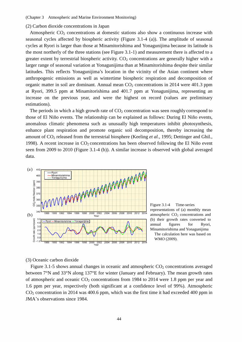
(Chapter 3 Atmospheric and Marine Environment Monitoring)
44
(2) Carbon dioxide concentrations in Japan Atmospheric CO2 concentrations at domestic stations also show a continuous increase with
seasonal cycles affected by biospheric activity (Figure 3.1-4 (a)). The amplitude of seasonal cycles at Ryori is larger than those at Minamitorishima and Yonagunijima because its latitude is the most northerly of the three stations (see Figure 3.1-1) and measurement there is affected to a greater extent by terrestrial biospheric activity. CO2 concentrations are generally higher with a larger range of seasonal variation at Yonagunijima than at Minamitorishima despite their similar latitudes. This reflects Yonagunijima’s location in the vicinity of the Asian continent where anthropogenic emissions as well as wintertime biospheric respiration and decomposition of organic matter in soil are dominant. Annual mean CO2 concentrations in 2014 were 401.3 ppm at Ryori, 399.5 ppm at Minamitorishima and 401.7 ppm at Yonagunijima, representing an increase on the previous year, and were the highest on record (values are preliminary estimations).
The periods in which a high growth rate of CO2 concentration was seen roughly correspond to those of El Niño events. The relationship can be explained as follows: During El Niño events, anomalous climatic phenomena such as unusually high temperatures inhibit photosynthesis, enhance plant respiration and promote organic soil decomposition, thereby increasing the amount of CO2 released from the terrestrial biosphere (Keeling et al., 1995; Dettinger and Ghil., 1998). A recent increase in CO2 concentrations has been observed following the El Niño event seen from 2009 to 2010 (Figure 3.1-4 (b)). A similar increase is observed with global averaged data.
(a) (b)
Figure 3.1-4 Time-series representations of (a) monthly mean atmospheric CO2 concentrations and (b) their growth rates converted to annual figures for Ryori, Minamitorishima and Yonagunijima
The calculation here was based on WMO (2009).
(3) Oceanic carbon dioxide Figure 3.1-5 shows annual changes in oceanic and atmospheric CO2 concentrations averaged
between 7°N and 33°N along 137°E for winter (January and February). The mean growth rates of atmospheric and oceanic CO2 concentrations from 1984 to 2014 were 1.8 ppm per year and 1.6 ppm per year, respectively (both significant at a confidence level of 99%). Atmospheric CO2 concentration in 2014 was 400.6 ppm, which was the first time it had exceeded 400 ppm in JMA’s observations since 1984.
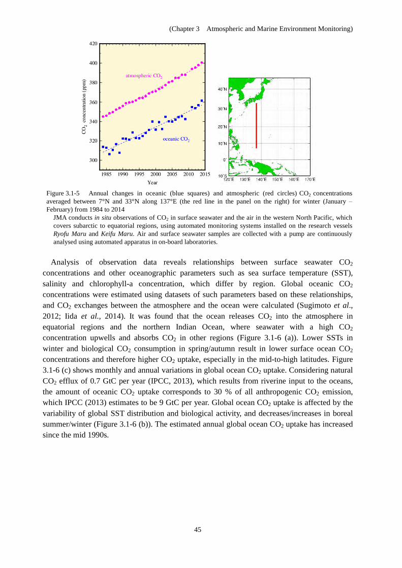
(Chapter 3 Atmospheric and Marine Environment Monitoring)
45
Figure 3.1-5 Annual changes in oceanic (blue squares) and atmospheric (red circles) CO2 concentrations averaged between 7°N and 33°N along 137°E (the red line in the panel on the right) for winter (January – February) from 1984 to 2014
JMA conducts in situ observations of CO2 in surface seawater and the air in the western North Pacific, which covers subarctic to equatorial regions, using automated monitoring systems installed on the research vessels Ryofu Maru and Keifu Maru. Air and surface seawater samples are collected with a pump are continuously analysed using automated apparatus in on-board laboratories.
Analysis of observation data reveals relationships between surface seawater CO2 concentrations and other oceanographic parameters such as sea surface temperature (SST), salinity and chlorophyll-a concentration, which differ by region. Global oceanic CO2 concentrations were estimated using datasets of such parameters based on these relationships, and CO2 exchanges between the atmosphere and the ocean were calculated (Sugimoto et al., 2012; Iida et al., 2014). It was found that the ocean releases CO2 into the atmosphere in equatorial regions and the northern Indian Ocean, where seawater with a high CO2 concentration upwells and absorbs CO2 in other regions (Figure 3.1-6 (a)). Lower SSTs in winter and biological CO2 consumption in spring/autumn result in lower surface ocean CO2 concentrations and therefore higher CO2 uptake, especially in the mid-to-high latitudes. Figure 3.1-6 (c) shows monthly and annual variations in global ocean CO2 uptake. Considering natural CO2 efflux of 0.7 GtC per year (IPCC, 2013), which results from riverine input to the oceans, the amount of oceanic CO2 uptake corresponds to 30 % of all anthropogenic CO2 emission, which IPCC (2013) estimates to be 9 GtC per year. Global ocean CO2 uptake is affected by the variability of global SST distribution and biological activity, and decreases/increases in boreal summer/winter (Figure 3.1-6 (b)). The estimated annual global ocean CO2 uptake has increased since the mid 1990s.
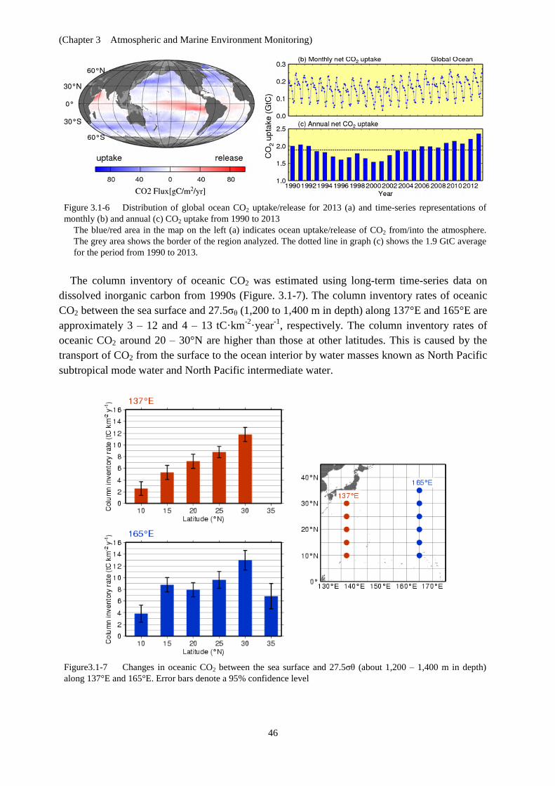
(Chapter 3 Atmospheric and Marine Environment Monitoring)
46
Figure 3.1-6 Distribution of global ocean CO2 uptake/release for 2013 (a) and time-series representations of monthly (b) and annual (c) CO2 uptake from 1990 to 2013
The blue/red area in the map on the left (a) indicates ocean uptake/release of CO2 from/into the atmosphere. The grey area shows the border of the region analyzed. The dotted line in graph (c) shows the 1.9 GtC average for the period from 1990 to 2013.
The column inventory of oceanic CO2 was estimated using long-term time-series data on
dissolved inorganic carbon from 1990s (Figure. 3.1-7). The column inventory rates of oceanic CO2 between the sea surface and 27.5σθ (1,200 to 1,400 m in depth) along 137°E and 165°E are approximately 3 – 12 and 4 – 13 tC·km-2·year-1, respectively. The column inventory rates of oceanic CO2 around 20 – 30°N are higher than those at other latitudes. This is caused by the transport of CO2 from the surface to the ocean interior by water masses known as North Pacific subtropical mode water and North Pacific intermediate water.
Figure3.1-7 Changes in oceanic CO2 between the sea surface and 27.5σθ (about 1,200 – 1,400 m in depth) along 137°E and 165°E. Error bars denote a 95% confidence level
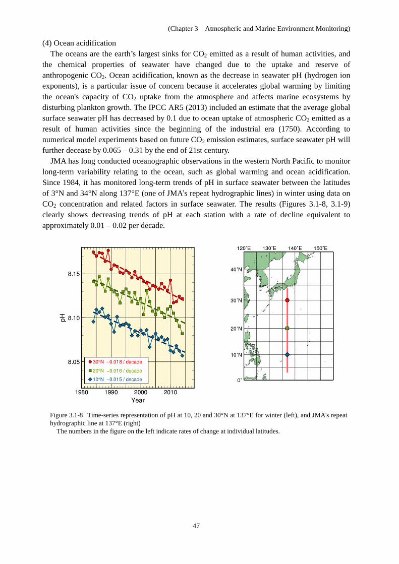
(Chapter 3 Atmospheric and Marine Environment Monitoring)
47
(4) Ocean acidification The oceans are the earth’s largest sinks for CO2 emitted as a result of human activities, and
the chemical properties of seawater have changed due to the uptake and reserve of anthropogenic CO2. Ocean acidification, known as the decrease in seawater pH (hydrogen ion exponents), is a particular issue of concern because it accelerates global warming by limiting the ocean's capacity of CO2 uptake from the atmosphere and affects marine ecosystems by disturbing plankton growth. The IPCC AR5 (2013) included an estimate that the average global surface seawater pH has decreased by 0.1 due to ocean uptake of atmospheric CO2 emitted as a result of human activities since the beginning of the industrial era (1750). According to numerical model experiments based on future CO2 emission estimates, surface seawater pH will further decease by 0.065 – 0.31 by the end of 21st century.
JMA has long conducted oceanographic observations in the western North Pacific to monitor long-term variability relating to the ocean, such as global warming and ocean acidification. Since 1984, it has monitored long-term trends of pH in surface seawater between the latitudes of 3°N and 34°N along 137°E (one of JMA’s repeat hydrographic lines) in winter using data on CO2 concentration and related factors in surface seawater. The results (Figures 3.1-8, 3.1-9) clearly shows decreasing trends of pH at each station with a rate of decline equivalent to approximately 0.01 – 0.02 per decade.
Figure 3.1-8 Time-series representation of pH at 10, 20 and 30°N at 137°E for winter (left), and JMA’s repeat hydrographic line at 137°E (right)
The numbers in the figure on the left indicate rates of change at individual latitudes.
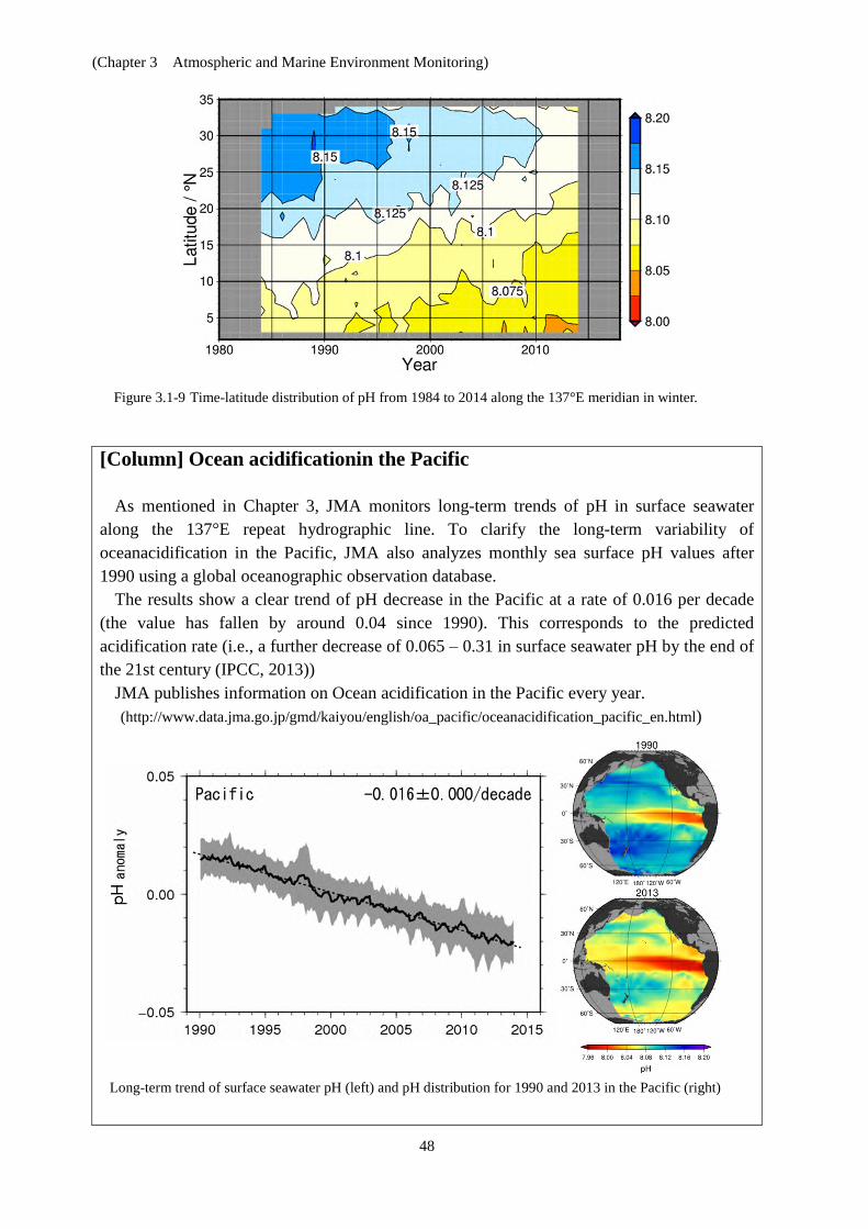
(Chapter 3 Atmospheric and Marine Environment Monitoring)
48
Figure 3.1-9 Time-latitude distribution of pH from 1984 to 2014 along the 137°E meridian in winter.
[Column] Ocean acidificationin the Pacific As mentioned in Chapter 3, JMA monitors long-term trends of pH in surface seawater
along the 137°E repeat hydrographic line. To clarify the long-term variability of oceanacidification in the Pacific, JMA also analyzes monthly sea surface pH values after 1990 using a global oceanographic observation database.
The results show a clear trend of pH decrease in the Pacific at a rate of 0.016 per decade (the value has fallen by around 0.04 since 1990). This corresponds to the predicted acidification rate (i.e., a further decrease of 0.065 – 0.31 in surface seawater pH by the end of the 21st century (IPCC, 2013))
JMA publishes information on Ocean acidification in the Pacific every year. (http://www.data.jma.go.jp/gmd/kaiyou/english/oa_pacific/oceanacidification_pacific_en.html)
Long-term trend of surface seawater pH (left) and pH distribution for 1990 and 2013 in the Pacific (right)
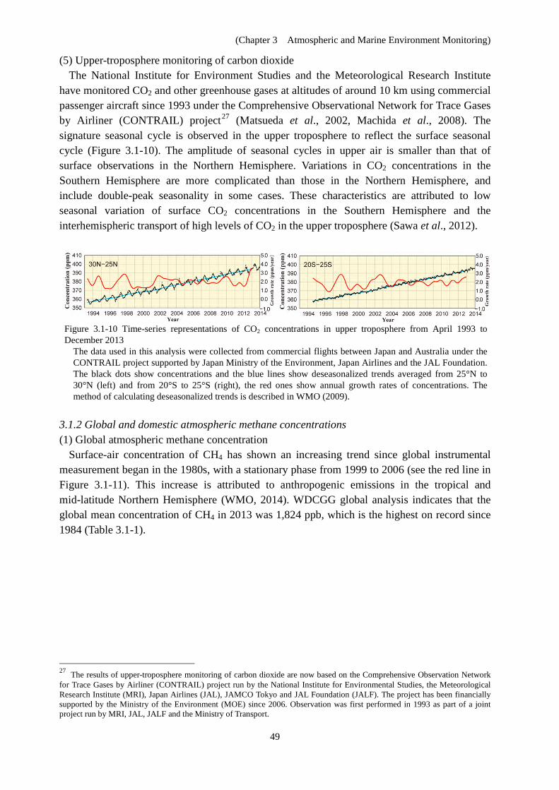
(Chapter 3 Atmospheric and Marine Environment Monitoring)
49
(5) Upper-troposphere monitoring of carbon dioxide The National Institute for Environment Studies and the Meteorological Research Institute
have monitored CO2 and other greenhouse gases at altitudes of around 10 km using commercial passenger aircraft since 1993 under the Comprehensive Observational Network for Trace Gases by Airliner (CONTRAIL) project27 (Matsueda et al., 2002, Machida et al., 2008). The signature seasonal cycle is observed in the upper troposphere to reflect the surface seasonal cycle (Figure 3.1-10). The amplitude of seasonal cycles in upper air is smaller than that of surface observations in the Northern Hemisphere. Variations in CO2 concentrations in the Southern Hemisphere are more complicated than those in the Northern Hemisphere, and include double-peak seasonality in some cases. These characteristics are attributed to low seasonal variation of surface CO2 concentrations in the Southern Hemisphere and the interhemispheric transport of high levels of CO2 in the upper troposphere (Sawa et al., 2012).
Figure 3.1-10 Time-series representations of CO2 concentrations in upper troposphere from April 1993 to December 2013
The data used in this analysis were collected from commercial flights between Japan and Australia under the CONTRAIL project supported by Japan Ministry of the Environment, Japan Airlines and the JAL Foundation. The black dots show concentrations and the blue lines show deseasonalized trends averaged from 25°N to 30°N (left) and from 20°S to 25°S (right), the red ones show annual growth rates of concentrations. The method of calculating deseasonalized trends is described in WMO (2009).
3.1.2 Global and domestic atmospheric methane concentrations (1) Global atmospheric methane concentration
Surface-air concentration of CH4 has shown an increasing trend since global instrumental measurement began in the 1980s, with a stationary phase from 1999 to 2006 (see the red line in Figure 3.1-11). This increase is attributed to anthropogenic emissions in the tropical and mid-latitude Northern Hemisphere (WMO, 2014). WDCGG global analysis indicates that the global mean concentration of CH4 in 2013 was 1,824 ppb, which is the highest on record since 1984 (Table 3.1-1).
27 The results of upper-troposphere monitoring of carbon dioxide are now based on the Comprehensive Observation Network for Trace Gases by Airliner (CONTRAIL) project run by the National Institute for Environmental Studies, the Meteorological Research Institute (MRI), Japan Airlines (JAL), JAMCO Tokyo and JAL Foundation (JALF). The project has been financially supported by the Ministry of the Environment (MOE) since 2006. Observation was first performed in 1993 as part of a joint project run by MRI, JAL, JALF and the Ministry of Transport.

(Chapter 3 Atmospheric and Marine Environment Monitoring)
50
Figure 3.1-11 Time-series representation of global atmospheric monthly-averaged CH4 concentration (blue line) and its deseasonalized trend (red line) (WMO, 2014)
The analysis was performed using data archived by the WDCGG. The deseasonalized trend calculation was based on WMO (2009).
Concentrations show a sharp decline southward from the mid- and high latitudes of the Northern Hemisphere to the Southern Hemisphere. This is because land areas in the Northern Hemisphere are home to major sources of CH4, which reacts with OH radicals28 and is transported to the Southern Hemisphere. Seasonal variations with a summer decrease are also apparent because large amounts of CH4 are removed through chemical reaction with OH radicals, whose presence increases in summer due to the effects of intensified ultraviolet radiation (Figure 3.1-12).
Figure 3.1-12 Monthly variations in zonally averaged atmospheric CH4 concentrations
This analysis was performed using data archived by the WDCGG. The calculation was based on WMO (2009).
Atmospheric CH4 concentration has shown a significant increase since the industrial era at a rate much higher than that of atmospheric CO2 (Table 3.1-1). This is attributable to larger anthropogenic emissions than those from natural sources as compared to the situation for CO2. The characteristics of CH4 variability have not yet been fully elucidated in quantitative terms because it is complicated by emissions from human activities, natural emissions from wetlands, and atmospheric chemical removal. To enhance understanding of the situation, the global CH4 observation network needs to be improved. (2) Methane concentration in Japan
The level of atmospheric CH4 concentration is the highest at Ryori, which has the most northerly latitude of the three JMA stations (Figure 3.1-13 (a)). This tendency is also common to hemispheric characteristics. The seasonal cycle exhibits a reduction in summer and an 28 OH radical is a highly reactive chemical generated by the reaction of the oxygen atom and water vapor contained in air, where the oxygen atom is derived from ozone by ultraviolet photolysis. In low latitudes, it is abundant produced by plenty of ultraviolet radiation and water vapor.
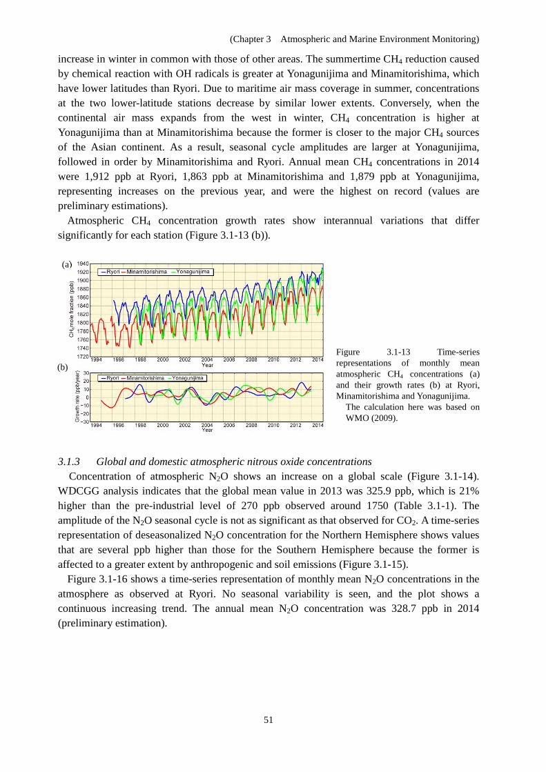
(Chapter 3 Atmospheric and Marine Environment Monitoring)
51
increase in winter in common with those of other areas. The summertime CH4 reduction caused by chemical reaction with OH radicals is greater at Yonagunijima and Minamitorishima, which have lower latitudes than Ryori. Due to maritime air mass coverage in summer, concentrations at the two lower-latitude stations decrease by similar lower extents. Conversely, when the continental air mass expands from the west in winter, CH4 concentration is higher at Yonagunijima than at Minamitorishima because the former is closer to the major CH4 sources of the Asian continent. As a result, seasonal cycle amplitudes are larger at Yonagunijima, followed in order by Minamitorishima and Ryori. Annual mean CH4 concentrations in 2014 were 1,912 ppb at Ryori, 1,863 ppb at Minamitorishima and 1,879 ppb at Yonagunijima, representing increases on the previous year, and were the highest on record (values are preliminary estimations).
Atmospheric CH4 concentration growth rates show interannual variations that differ significantly for each station (Figure 3.1-13 (b)). (a)
(b)
Figure 3.1-13 Time-series representations of monthly mean atmospheric CH4 concentrations (a) and their growth rates (b) at Ryori, Minamitorishima and Yonagunijima.
The calculation here was based on WMO (2009).
3.1.3 Global and domestic atmospheric nitrous oxide concentrations
Concentration of atmospheric N2O shows an increase on a global scale (Figure 3.1-14). WDCGG analysis indicates that the global mean value in 2013 was 325.9 ppb, which is 21% higher than the pre-industrial level of 270 ppb observed around 1750 (Table 3.1-1). The amplitude of the N2O seasonal cycle is not as significant as that observed for CO2. A time-series representation of deseasonalized N2O concentration for the Northern Hemisphere shows values that are several ppb higher than those for the Southern Hemisphere because the former is affected to a greater extent by anthropogenic and soil emissions (Figure 3.1-15).
Figure 3.1-16 shows a time-series representation of monthly mean N2O concentrations in the atmosphere as observed at Ryori. No seasonal variability is seen, and the plot shows a continuous increasing trend. The annual mean N2O concentration was 328.7 ppb in 2014 (preliminary estimation).
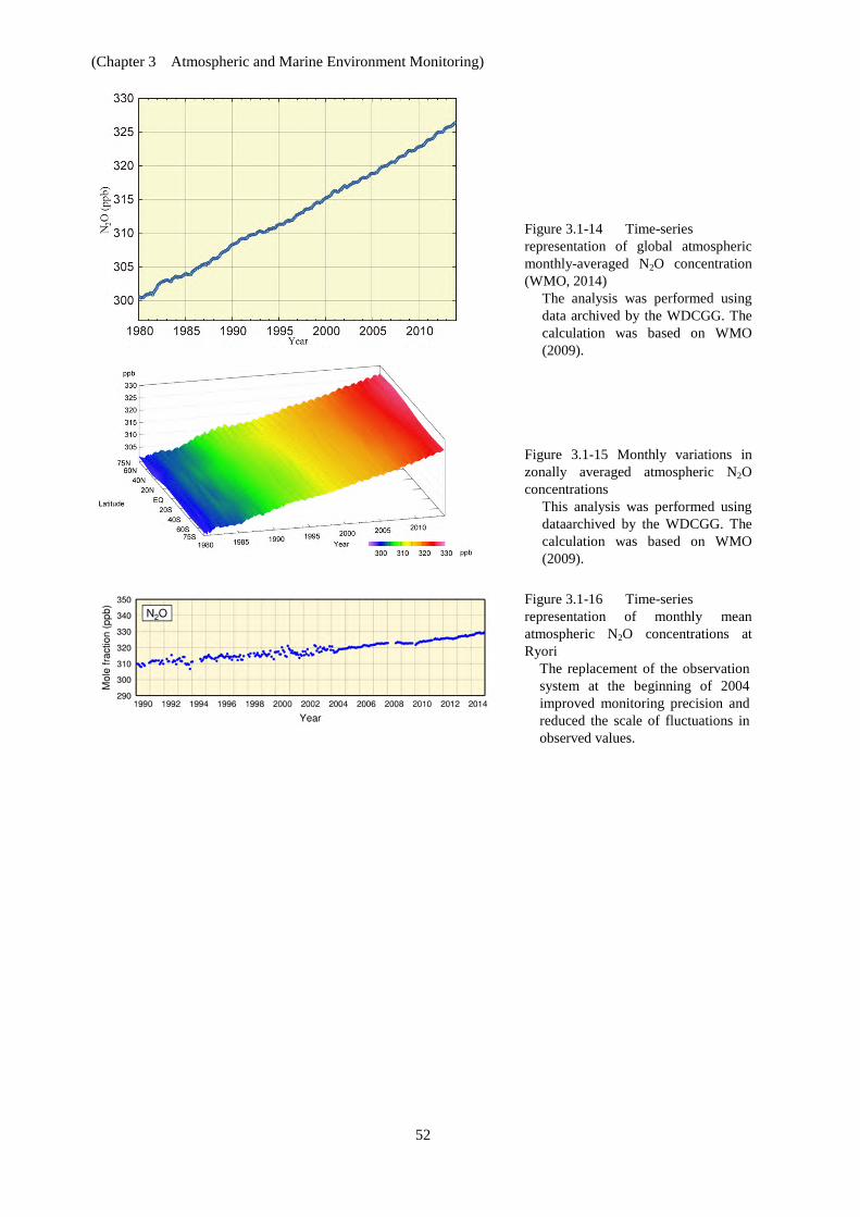
(Chapter 3 Atmospheric and Marine Environment Monitoring)
52
Figure 3.1-14 Time-series representation of global atmospheric monthly-averaged N2O concentration (WMO, 2014)
The analysis was performed using data archived by the WDCGG. The calculation was based on WMO (2009).
Figure 3.1-15 Monthly variations in zonally averaged atmospheric N2O concentrations
This analysis was performed using dataarchived by the WDCGG. The calculation was based on WMO (2009).
Figure 3.1-16 Time-series representation of monthly mean atmospheric N2O concentrations at Ryori
The replacement of the observation system at the beginning of 2004 improved monitoring precision and reduced the scale of fluctuations in observed values.
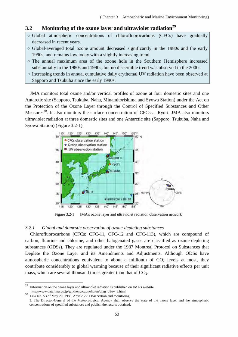
(Chapter 3 Atmospheric and Marine Environment Monitoring)
53
3.2 Monitoring of the ozone layer and ultraviolet radiation29
○ Global atmospheric concentrations of chlorofluorocarbons (CFCs) have gradually decreased in recent years.
○ Global-averaged total ozone amount decreased significantly in the 1980s and the early 1990s, and remains low today with a slightly increasing trend.
○ The annual maximum area of the ozone hole in the Southern Hemisphere increased substantially in the 1980s and 1990s, but no discernible trend was observed in the 2000s.
○ Increasing trends in annual cumulative daily erythemal UV radiation have been observed at Sapporo and Tsukuba since the early 1990s.
JMA monitors total ozone and/or vertical profiles of ozone at four domestic sites and one
Antarctic site (Sapporo, Tsukuba, Naha, Minamitorishima and Syowa Station) under the Act on the Protection of the Ozone Layer through the Control of Specified Substances and Other Measures30. It also monitors the surface concentration of CFCs at Ryori. JMA also monitors ultraviolet radiation at three domestic sites and one Antarctic site (Sapporo, Tsukuba, Naha and Syowa Station) (Figure 3.2-1).
Figure 3.2-1 JMA’s ozone layer and ultraviolet radiation observation network
3.2.1 Global and domestic observation of ozone-depleting substances
Chlorofluorocarbons (CFCs: CFC-11, CFC-12 and CFC-113), which are compound of carbon, fluorine and chlorine, and other halogenated gases are classified as ozone-depleting substances (ODSs). They are regulated under the 1987 Montreal Protocol on Substances that Deplete the Ozone Layer and its Amendments and Adjustments. Although ODSs have atmospheric concentrations equivalent to about a millionth of CO2 levels at most, they contribute considerably to global warming because of their significant radiative effects per unit mass, which are several thousand times greater than that of CO2.
29 Information on the ozone layer and ultraviolet radiation is published on JMA’s website.
http://www.data.jma.go.jp/gmd/env/ozonehp/en/diag_o3uv_e.html 30 Law No. 53 of May 20, 1988, Article 22: Observation and monitoring
1. The Director-General of the Meteorological Agency shall observe the state of the ozone layer and the atmospheric concentrations of specified substances and publish the results obtained.
E N

(Chapter 3 Atmospheric and Marine Environment Monitoring)
54
(1) Global concentrations of ozone-depleting substances Global concentrations of atmospheric CFCs increased rapidly until the 1980s. However,
since the 1990s, falling rates of increase or a decreasing tendency have been dominant (Figure 3.2-2) due to the effect of the Montreal Protocol. Maximum concentrations of CFC-11 were observed from 1992 to 1994, and have shown a decreasing tendency since then. Concentrations of CFC-12 increased until around 2005, and have also shown a decreasing tendency since then. The trend for CFC-113 concentrations and variations are almost the same as those of CFC-11, peaking around 1993 – 1994 in the Northern Hemisphere and around 1997 in the Southern Hemishpere. Differences in the concentrationsof these gases between the Northern Hemisphere (where most emission sources are located) and the Southern Hemisphere (which has significantly fewer sources) tended to be smaller in the 2000s than in the 1980s and 1990s. These results show the gradual appearance of a positive effect from CFC emission control efforts in readings of atmospheric CFC concentrations.
Figure 3.2-2 Time series of the monthly mean concentrations of CFCs
CFC-11 (upper left), CFC-12 (upper right) and CFC-113 (lower left). These figures were produced using data archived in the WDCGG.
(2) Ozone-depleting substances in Japan
In line with global observations, concentrations of CFC-11, CFC-12 and CFC-113 at Ryori have all decreased since reaching peaks in different periods (Figure 3.2-3). The concentration of CFC-11 peaked at about 270 ppt in 1993 – 1994, and has decreased since then. CFC-11 showed a distinct maximum of concentrations when temperatures were high during the summer of 2011, which may be attributable to effective leakage from damaged polyurethane insulation foam related to the Tohoku earthquake and tsunami of 11 March 2011 (Saito et al., 2015). CFC-12 concentration increased rapidly until 1995 and continued to rise slowly until 2005, but has shown a gradual decrease since then. The concentration of CFC-113 showed no clear trend until 2001 and decreased gradually thereafter.
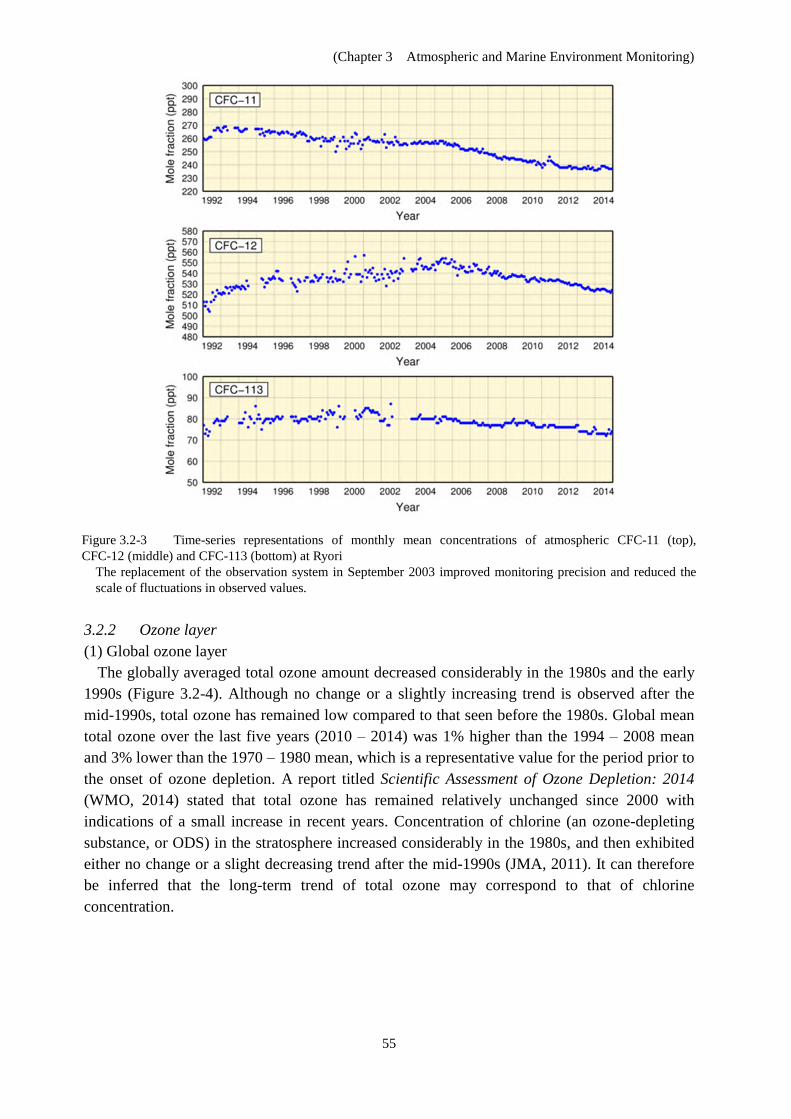
(Chapter 3 Atmospheric and Marine Environment Monitoring)
55
Figure 3.2-3 Time-series representations of monthly mean concentrations of atmospheric CFC-11 (top), CFC-12 (middle) and CFC-113 (bottom) at Ryori
The replacement of the observation system in September 2003 improved monitoring precision and reduced the scale of fluctuations in observed values.
3.2.2 Ozone layer (1) Global ozone layer
The globally averaged total ozone amount decreased considerably in the 1980s and the early 1990s (Figure 3.2-4). Although no change or a slightly increasing trend is observed after the mid-1990s, total ozone has remained low compared to that seen before the 1980s. Global mean total ozone over the last five years (2010 – 2014) was 1% higher than the 1994 – 2008 mean and 3% lower than the 1970 – 1980 mean, which is a representative value for the period prior to the onset of ozone depletion. A report titled Scientific Assessment of Ozone Depletion: 2014 (WMO, 2014) stated that total ozone has remained relatively unchanged since 2000 with indications of a small increase in recent years. Concentration of chlorine (an ozone-depleting substance, or ODS) in the stratosphere increased considerably in the 1980s, and then exhibited either no change or a slight decreasing trend after the mid-1990s (JMA, 2011). It can therefore be inferred that the long-term trend of total ozone may correspond to that of chlorine concentration.
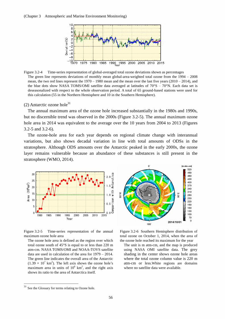
(Chapter 3 Atmospheric and Marine Environment Monitoring)
56
Figure 3.2-4 Time-series representation of global-averaged total ozone deviations shown as percentages
The green line represents deviations of monthly mean global-area-weighted total ozone from the 1994 – 2008 mean, the two red lines represent the 1970 – 1980 mean and the mean over the last five years (2010 – 2014), and the blue dots show NASA TOMS/OMI satellite data averaged at latitudes of 70°S – 70°N. Each data set is deseasonalized with respect to the whole observation period. A total of 65 ground-based stations were used for this calculation (55 in the Northern Hemisphere and 10 in the Southern Hemisphere).
(2) Antarctic ozone hole31
The annual maximum area of the ozone hole increased substantially in the 1980s and 1990s, but no discernible trend was observed in the 2000s (Figure 3.2-5). The annual maximum ozone hole area in 2014 was equivalent to the average over the 10 years from 2004 to 2013 (Figures 3.2-5 and 3.2-6).
The ozone-hole area for each year depends on regional climate change with interannual variations, but also shows decadal variation in line with total amounts of ODSs in the stratosphere. Although ODS amounts over the Antarctic peaked in the early 2000s, the ozone layer remains vulnerable because an abundance of these substances is still present in the stratosphere (WMO, 2014).
Figure 3.2-5 Time-series representation of the annual maximum ozone hole area
The ozone hole area is defined as the region over which total ozone south of 45°S is equal to or less than 220 m atm-cm. NASA TOMS/OMI and NOAA-TOVS satellite data are used in calculation of the area for 1979 – 2014. The green line indicates the overall area of the Antarctic (1.39 × 10⁷ km2). The left axis shows the ozone hole’s maximum area in units of 106 km2, and the right axis shows its ratio to the area of Antarctica itself.
Figure 3.2-6 Southern Hemisphere distribution of total ozone on October 1, 2014, when the area of the ozone hole reached its maximum for the year
The unit is m atm-cm, and the map is produced using NASA OMI satellite data. The grey shading in the center shows ozone hole areas where the total ozone column value is 220 m atm-cm or less.White regions are domains where no satellite data were available.
31 See the Glossary for terms relating to Ozone hole.
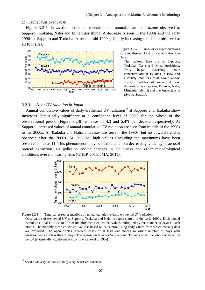
(Chapter 3 Atmospheric and Marine Environment Monitoring)
57
(3) Ozone layer over Japan Figure 3.2-7 shows time-series representations of annual-mean total ozone observed at
Sapporo, Tsukuba, Naha and Minamitorishima. A decrease is seen in the 1980s and the early 1990s at Sapporo and Tsukuba. After the mid-1990s, slightly increasing trends are observed at all four sites.
Figure 3.2-7 Time-series representations of annual-mean total ozone at stations in Japan
The stations here are at Sapporo, Tsukuba, Naha and Minamitorishima. JMA began observing ozone concentrations at Tsukuba in 1957 and currently monitors total ozone and/or vertical profiles of ozone at four domestic sites (Sapporo, Tsukuba, Naha, Minamitorishima) and one Antarctic site (Syowa Station).
3.2.3 Solar UV radiation in Japan Annual cumulative values of daily erythemal UV radiation32 at Sapporo and Tsukuba show
increases (statistically significant at a confidence level of 99%) for the whole of the observational period (Figure 3.2-8) at ratios of 4.3 and 5.4% per decade, respectively. At Sapporo, increased values of annual cumulative UV radiation are seen from middle of the 1990s to the 2000s. At Tsukuba and Naha, increases are seen in the 1990s, but no upward trend is observed after the 2000s. At Tsukuba, high values (including the maximum) have been observed since 2011. This phenomenon may be attributable to a decreasing tendency of aerosol optical extinction, air pollution and/or changes in cloudiness and other meteorological conditions over monitoring sites (UNEP, 2015; JMA, 2011).
Figure 3.2-8 Time-series representations of annual cumulative daily erythemal UV radiation Observation of erythemal UV at Sapporo, Tsukuba and Naha in Japan started in the early 1990s. Each annual cumulative total is calculated from monthly-mean equivalent values multiplied by the number of days in each month. The monthly-mean equivalent value is based on calculation using daily values from which missing data are excluded. The open circles represent cases of at least one month in which number of days with measurements are less than 20 days. The regression lines for Sapporo and Tsukuba cover the whole observation period (statistically significant at a confidence level of 99%).
32 See the Glossary for terms relating to erythemal UV radiation.
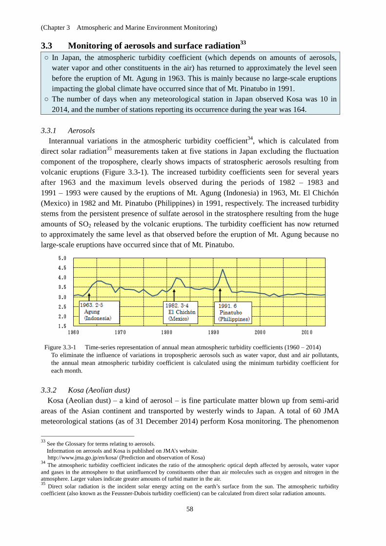
(Chapter 3 Atmospheric and Marine Environment Monitoring)
58
3.3 Monitoring of aerosols and surface radiation33 ○ In Japan, the atmospheric turbidity coefficient (which depends on amounts of aerosols,
water vapor and other constituents in the air) has returned to approximately the level seen before the eruption of Mt. Agung in 1963. This is mainly because no large-scale eruptions impacting the global climate have occurred since that of Mt. Pinatubo in 1991.
○ The number of days when any meteorological station in Japan observed Kosa was 10 in 2014, and the number of stations reporting its occurrence during the year was 164.
3.3.1 Aerosols Interannual variations in the atmospheric turbidity coefficient34, which is calculated from
direct solar radiation35 measurements taken at five stations in Japan excluding the fluctuation component of the troposphere, clearly shows impacts of stratospheric aerosols resulting from volcanic eruptions (Figure 3.3-1). The increased turbidity coefficients seen for several years after 1963 and the maximum levels observed during the periods of 1982 – 1983 and 1991 – 1993 were caused by the eruptions of Mt. Agung (Indonesia) in 1963, Mt. El Chichón (Mexico) in 1982 and Mt. Pinatubo (Philippines) in 1991, respectively. The increased turbidity stems from the persistent presence of sulfate aerosol in the stratosphere resulting from the huge amounts of SO2 released by the volcanic eruptions. The turbidity coefficient has now returned to approximately the same level as that observed before the eruption of Mt. Agung because no large-scale eruptions have occurred since that of Mt. Pinatubo.
Figure 3.3-1 Time-series representation of annual mean atmospheric turbidity coefficients (1960 – 2014)
To eliminate the influence of variations in tropospheric aerosols such as water vapor, dust and air pollutants, the annual mean atmospheric turbidity coefficient is calculated using the minimum turbidity coefficient for each month.
3.3.2 Kosa (Aeolian dust)
Kosa (Aeolian dust) – a kind of aerosol – is fine particulate matter blown up from semi-arid areas of the Asian continent and transported by westerly winds to Japan. A total of 60 JMA meteorological stations (as of 31 December 2014) perform Kosa monitoring. The phenomenon
33 See the Glossary for terms relating to aerosols. Information on aerosols and Kosa is published on JMA’s website.
http://www.jma.go.jp/en/kosa/ (Prediction and observation of Kosa) 34 The atmospheric turbidity coefficient indicates the ratio of the atmospheric optical depth affected by aerosols, water vapor and gases in the atmosphere to that uninfluenced by constituents other than air molecules such as oxygen and nitrogen in the atmosphere. Larger values indicate greater amounts of turbid matter in the air. 35 Direct solar radiation is the incident solar energy acting on the earth’s surface from the sun. The atmospheric turbidity coefficient (also known as the Feussner-Dubois turbidity coefficient) can be calculated from direct solar radiation amounts.
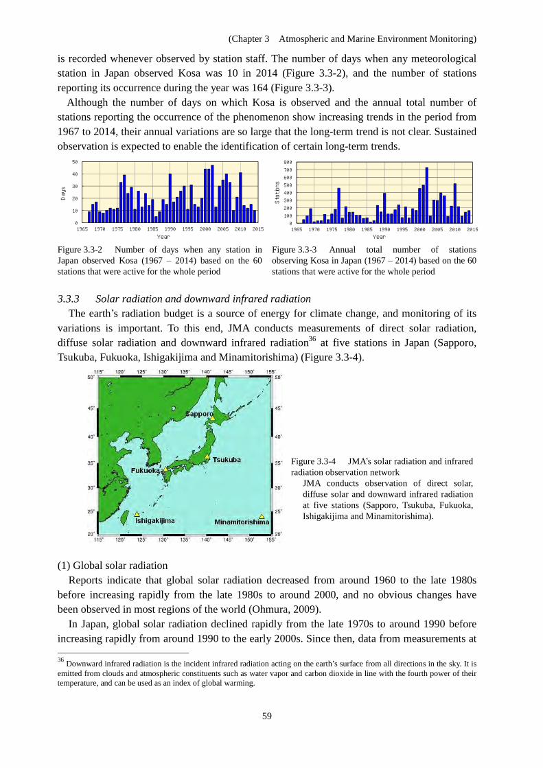
(Chapter 3 Atmospheric and Marine Environment Monitoring)
59
is recorded whenever observed by station staff. The number of days when any meteorological station in Japan observed Kosa was 10 in 2014 (Figure 3.3-2), and the number of stations reporting its occurrence during the year was 164 (Figure 3.3-3).
Although the number of days on which Kosa is observed and the annual total number of stations reporting the occurrence of the phenomenon show increasing trends in the period from 1967 to 2014, their annual variations are so large that the long-term trend is not clear. Sustained observation is expected to enable the identification of certain long-term trends.
3.3.3 Solar radiation and downward infrared radiation The earth’s radiation budget is a source of energy for climate change, and monitoring of its
variations is important. To this end, JMA conducts measurements of direct solar radiation, diffuse solar radiation and downward infrared radiation36 at five stations in Japan (Sapporo, Tsukuba, Fukuoka, Ishigakijima and Minamitorishima) (Figure 3.3-4).
Figure 3.3-4 JMA’s solar radiation and infrared radiation observation network
JMA conducts observation of direct solar, diffuse solar and downward infrared radiation at five stations (Sapporo, Tsukuba, Fukuoka, Ishigakijima and Minamitorishima).
(1) Global solar radiation
Reports indicate that global solar radiation decreased from around 1960 to the late 1980s before increasing rapidly from the late 1980s to around 2000, and no obvious changes have been observed in most regions of the world (Ohmura, 2009).
In Japan, global solar radiation declined rapidly from the late 1970s to around 1990 before increasing rapidly from around 1990 to the early 2000s. Since then, data from measurements at 36 Downward infrared radiation is the incident infrared radiation acting on the earth’s surface from all directions in the sky. It is emitted from clouds and atmospheric constituents such as water vapor and carbon dioxide in line with the fourth power of their temperature, and can be used as an index of global warming.
Figure 3.3-2 Number of days when any station in Japan observed Kosa (1967 – 2014) based on the 60 stations that were active for the whole period
Figure 3.3-3 Annual total number of stations observing Kosa in Japan (1967 – 2014) based on the 60 stations that were active for the whole period
0
10
20
30
40
50
1965 1970 1975 1980 1985 1990 1995 2000 2005 2010 2015
Days
Year
0
100
200
300
400
500
600
700
800
1965 1970 1975 1980 1985 1990 1995 2000 2005 2010 2015
Stations
Year
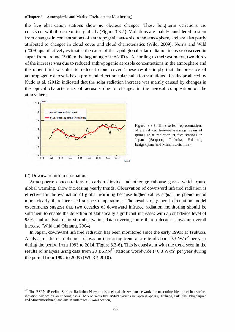
(Chapter 3 Atmospheric and Marine Environment Monitoring)
60
the five observation stations show no obvious changes. These long-term variations are consistent with those reported globally (Figure 3.3-5). Variations are mainly considered to stem from changes in concentrations of anthropogenic aerosols in the atmosphere, and are also partly attributed to changes in cloud cover and cloud characteristics (Wild, 2009). Norris and Wild (2009) quantitatively estimated the cause of the rapid global solar radiation increase observed in Japan from around 1990 to the beginning of the 2000s. According to their estimates, two thirds of the increase was due to reduced anthropogenic aerosols concentrations in the atmosphere and the other third was due to reduced cloud cover. These results imply that the presence of anthropogenic aerosols has a profound effect on solar radiation variations. Results produced by Kudo et al. (2012) indicated that the solar radiation increase was mainly caused by changes in the optical characteristics of aerosols due to changes in the aerosol composition of the atmosphere.
Figure 3.3-5 Time-series representations of annual and five-year-running means of global solar radiation at five stations in Japan (Sapporo, Tsukuba, Fukuoka, Ishigakijima and Minamitorishima)
(2) Downward infrared radiation Atmospheric concentrations of carbon dioxide and other greenhouse gases, which cause
global warming, show increasing yearly trends. Observation of downward infrared radiation is effective for the evaluation of global warming because higher values signal the phenomenon more clearly than increased surface temperatures. The results of general circulation model experiments suggest that two decades of downward infrared radiation monitoring should be sufficient to enable the detection of statistically significant increases with a confidence level of 95%, and analysis of in situ observation data covering more than a decade shows an overall increase (Wild and Ohmura, 2004).
In Japan, downward infrared radiation has been monitored since the early 1990s at Tsukuba. Analysis of the data obtained shows an increasing trend at a rate of about 0.3 W/m2 per year during the period from 1993 to 2014 (Figure 3.3-6). This is consistent with the trend seen in the results of analysis using data from 20 BSRN37 stations worldwide (+0.3 W/m2 per year during the period from 1992 to 2009) (WCRP, 2010).
37 The BSRN (Baseline Surface Radiation Network) is a global observation network for measuring high-precision surface radiation balance on an ongoing basis. JMA operates five BSRN stations in Japan (Sapporo, Tsukuba, Fukuoka, Ishigakijima and Minamitorishima) and one in Antarctica (Syowa Station).
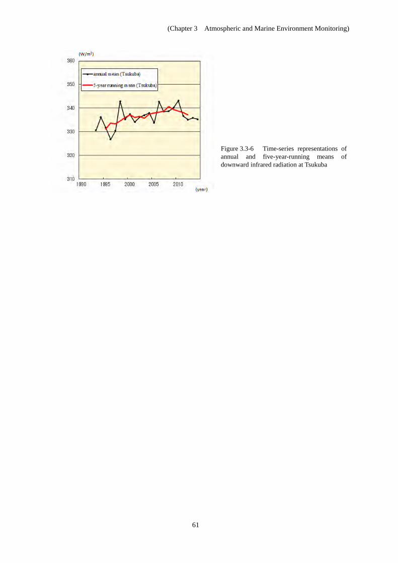
(Chapter 3 Atmospheric and Marine Environment Monitoring)
61
Figure 3.3-6 Time-series representations of annual and five-year-running means of downward infrared radiation at Tsukuba
62
Explanatory note on detection of statistical significance in long-term trends
Meteorological observation data, including those relating to temperature and precipitation, are subject to large amplitude fluctuations due to the influence of atmospheric and oceanic dynamics on a broad spectrum of spatial and temporal scales. To examine the possible presence of long-term climate system trends associated with global warming in consideration of natural variability, raw climate data need to be converted into suitable statistical time-series representations and subjected to statistical testing in order to highlight the likelihood of systematic temporal trends that cannot be explained by random variability alone. When the results of such testing allow reasonable conclusion that random variability is unlikely to be the sole factor at work, a change is described as statistically significant.
In this report, the likelihood of a systematic long-term change existing in a time-series representation is based on the results of statistical significance testing performed at confidence levels of 99, 95 and 90%. The following terminology summary describes each level:
The following statistical methods are applied for the data used in this report:
i) For statistical variables whose annual fluctuation component can be assumed to follow
normal distribution For temperature anomalies, trend-removed annual variability data are expected to
approximately follow normal distribution. T-testing is performed for statistical variables assumed to be normally distributed using a coefficient of correlation between years and values.
ii) For statistical variables whose annual fluctuation component cannot be assumed to follow
normal distribution The assumption of normality may not be applicable to frequency statistics regarding weather
conditions, including those for extremely warm days, tropical nights and hourly precipitation amounts exceeding 50 mm. Accordingly, non-parametric testing, which does not depend on underlying assumptions about distribution, is applied to such variables.
It should be noted that statistical tests are in theory inevitably susceptible to the establishment
of false conclusions even if the results indicate a statistically significant trend. Even outcomes
Level of confidence
Term
≥ 99% Virtually certain to have increased/decreased (statistically significant at a confidence level of 99%)
≥ 95% Extremely likely to have increased/decreased (statistically significant at a confidence level of 95%)
≥ 90% Very likely to have increased/decreased (statistically significant at a confidence level of 90%)
< 90% No discernible trend
63
indicating statistical significance at confidence levels of 90, 95 or 99% imply that there are small inherent probabilities of up to 10, 5 and 1%, respectively, of the significance being erroneously detected when in fact the observed long-term change occurred by mere random chance. Conversely, when a systematic long-term change actually exists, statistical testing may fail to detect the significance correctly. In general, test results are not considered highly stable if they are based on observation records that are temporally limited, influenced by large annual fluctuations/rare events or subject to change when new observations are added to a data sequence. Readers are encouraged to interpret the analytical results presented in the report appropriately with due note of these considerations.
64
Glossary
Aerosols Aerosols are airborne solids or liquids in fine particle form. Their many types include
particles of natural origin blown up from land/sea surfaces, anthropogenic particles and secondary aerosols formed from anthropogenic and biogenic precursors. In addition to absorbing and scattering sunlight, they also provide condensation nuclei for clouds. Particle matter 2.5 (PM2.5) is the name given to aerosol particles measuring 2.5 micrometers or less in diameter (about 30 times thinner than a human hair), and is considered to have possible adverse effects on human health when inhaled. Anthropogenic
Resulting from or produced by human activities. Arctic Oscillation
The Arctic Oscillation (AO) is a major atmospheric circulation variation exhibiting an annular pattern of sea-level pressure anomalies in a seesaw fashion with one sign over the Arctic region and the opposite sign over the mid-latitudes. Its negative phase, which is characterized by positive and negative sea-level pressure anomalies over the Arctic region and the mid-latitudes, respectively, helps cold Arctic air move into the mid-latitudes. The positive phase, whose sea-level pressure anomaly pattern is reversed, keeps Arctic air over the Arctic region. Erythemal UV radiation
Erythema is sunburn – a reddening of the skin resulting from continuous exposure to ultraviolet (UV) rays present in solar radiation. It is known that excessive erythema and long-term exposure to the sun can cause human health problems such as a high incidence of skin cancer and cataracts. Erythemal UV radiation is widely used as a scale of UV radiation for evaluation of its effects on the human body, and is calculated in consideration of various influences depending on wavelength. Extreme climate event
In general, an extreme climate event is recognized as an unusually severe or rare climate event creating disaster conditions or exerting significant socio-economic influence. The definition includes severe weather conditions covering periods ranging from only a few hours (such as heavy rain or strong wind) to several months (such as drought or cold summer conditions). JMA defines extreme climate events as those occurring once every 30 years or longer. IPCC (Intergovernmental Panel on Climate Change)
The Intergovernmental Panel on Climate Change (IPCC) is an international organization established by the United Nations Environment Programme (UNEP) and the World Meteorological Organization (WMO) in 1988. It reviews and assesses scientific, technical and socio-economic information on climate change, the potential impacts of such change and related vulnerability, and options for adaptation and mitigation, in collaboration with scientists and experts on an international basis. The Panel’s reports highlight common understanding of such information to support political matters such as treaty negotiations on global warming.

65
Kosa (Aeolian dust) Kosa (Aeolian dust) is a meteorological phenomenon in which fine dust is blown up to an
altitude of several thousand meters by cyclonic or other wind systems from deserts or cropland in semi-arid areas of the Asian continent, and is transported over long distances by westerly winds, resulting in haze or dustfall in downstream areas. It is often observed between March and June in Japan and makes the sky yellow and hazy. Heavy Kosa can affect transportation by obstructing visibility.
Monsoon The term monsoon primarily refers to seasonally reversing winds, and by extension includes
related seasonal rainfall change with wet and dry phases. Monsoon climate regions where seasonal winds prevail are found in numerous places around the world, with a major one located over a broad area from the Asian continent to northern Australia.
Normals Normals represent climatic conditions at meteorological stations, and are used as a base to
evaluate meteorological variables (e.g., temperature, precipitation and sunshine duration) and produce generalizations (e.g., cool summer, warm winter and dry/wet months) for particular periods. JMA uses averages for the most recent three decades (currently 1981 – 2010) as normals, which are updated every decade in line with WMO Technical Regulations.
Terms relating to El Niño/La Niña phenomena El Niño/La Niña phenomena: an El Niño event is a phenomenon in which sea surface
temperatures (SSTs) are higher than normal across a wide region from the center of the equatorial Pacific to the area off the coast of Peru for a period from half a year to one and a half years. In contrast, a La Niña event is a phenomenon in which SSTs are lower than normal in the same area. Both occur every few years, and are associated with frequent extreme climate conditions worldwide.
JMA recognizes the occurrence of an El Niño event when the five-month running mean of SST deviations from the climatological mean (based on a sliding 30-year period averaged over the NINO.3 El Niño Monitoring Region (5ºN – 5ºS, 150ºW – 90ºW; Figure A)) remains above +0.5°C for a period of six months or more. Similarly, a La Niña event is recognized when the corresponding figure is below −0.5°C for the same area/period.
Figure B shows typical SST deviations from the normal during El Niño and La Niña events. The dark red and blue shading seen from the date line to the coast of South America indicates large deviations.
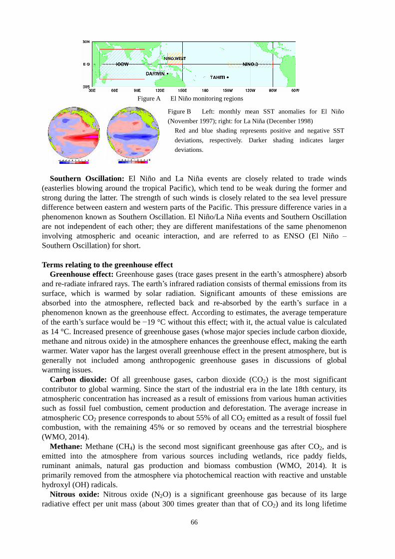
66
Figure B Left: monthly mean SST anomalies for El Niño (November 1997); right: for La Niña (December 1998)
Red and blue shading represents positive and negative SST deviations, respectively. Darker shading indicates larger deviations.
Southern Oscillation: El Niño and La Niña events are closely related to trade winds (easterlies blowing around the tropical Pacific), which tend to be weak during the former and strong during the latter. The strength of such winds is closely related to the sea level pressure difference between eastern and western parts of the Pacific. This pressure difference varies in a phenomenon known as Southern Oscillation. El Niño/La Niña events and Southern Oscillation are not independent of each other; they are different manifestations of the same phenomenon involving atmospheric and oceanic interaction, and are referred to as ENSO (El Niño – Southern Oscillation) for short. Terms relating to the greenhouse effect
Greenhouse effect: Greenhouse gases (trace gases present in the earth’s atmosphere) absorb and re-radiate infrared rays. The earth’s infrared radiation consists of thermal emissions from its surface, which is warmed by solar radiation. Significant amounts of these emissions are absorbed into the atmosphere, reflected back and re-absorbed by the earth’s surface in a phenomenon known as the greenhouse effect. According to estimates, the average temperature of the earth’s surface would be −19 °C without this effect; with it, the actual value is calculated as 14 °C. Increased presence of greenhouse gases (whose major species include carbon dioxide, methane and nitrous oxide) in the atmosphere enhances the greenhouse effect, making the earth warmer. Water vapor has the largest overall greenhouse effect in the present atmosphere, but is generally not included among anthropogenic greenhouse gases in discussions of global warming issues.
Carbon dioxide: Of all greenhouse gases, carbon dioxide (CO2) is the most significant contributor to global warming. Since the start of the industrial era in the late 18th century, its atmospheric concentration has increased as a result of emissions from various human activities such as fossil fuel combustion, cement production and deforestation. The average increase in atmospheric CO2 presence corresponds to about 55% of all CO2 emitted as a result of fossil fuel combustion, with the remaining 45% or so removed by oceans and the terrestrial biosphere (WMO, 2014).
Methane: Methane (CH4) is the second most significant greenhouse gas after CO2, and is emitted into the atmosphere from various sources including wetlands, rice paddy fields, ruminant animals, natural gas production and biomass combustion (WMO, 2014). It is primarily removed from the atmosphere via photochemical reaction with reactive and unstable hydroxyl (OH) radicals.
Nitrous oxide: Nitrous oxide (N2O) is a significant greenhouse gas because of its large radiative effect per unit mass (about 300 times greater than that of CO2) and its long lifetime
Figure A El Niño monitoring regions
℃
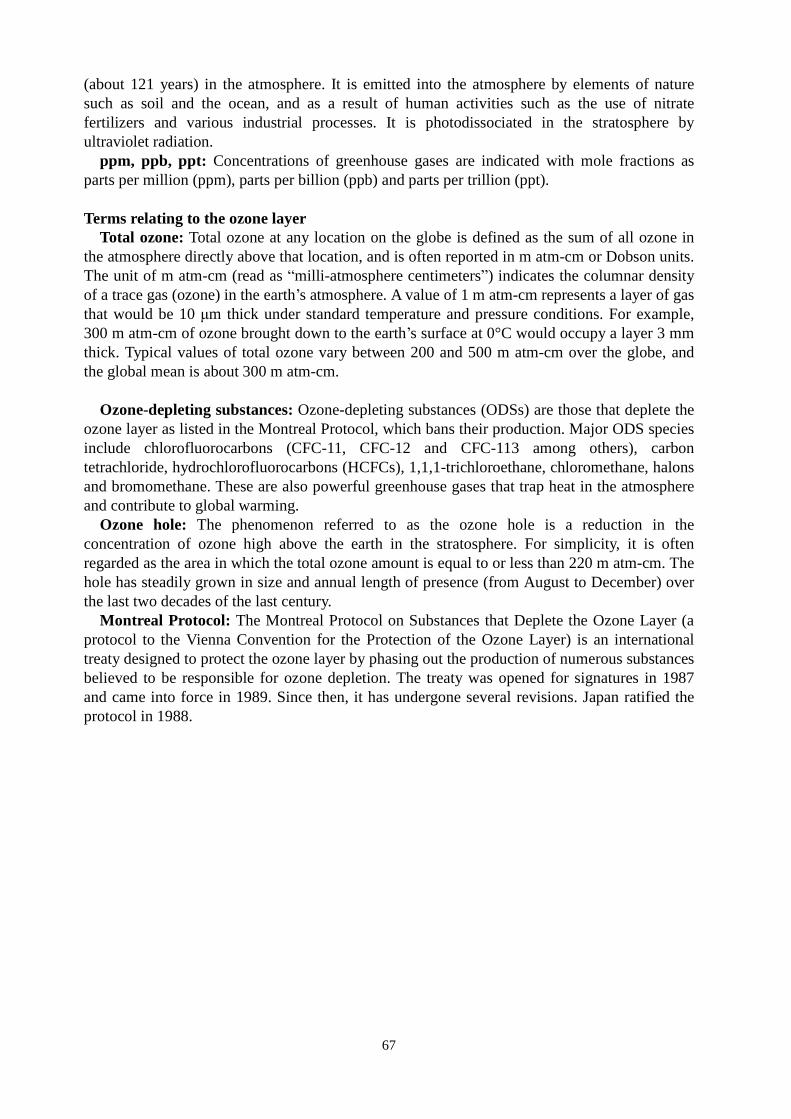
67
(about 121 years) in the atmosphere. It is emitted into the atmosphere by elements of nature such as soil and the ocean, and as a result of human activities such as the use of nitrate fertilizers and various industrial processes. It is photodissociated in the stratosphere by ultraviolet radiation.
ppm, ppb, ppt: Concentrations of greenhouse gases are indicated with mole fractions as parts per million (ppm), parts per billion (ppb) and parts per trillion (ppt). Terms relating to the ozone layer
Total ozone: Total ozone at any location on the globe is defined as the sum of all ozone in the atmosphere directly above that location, and is often reported in m atm-cm or Dobson units. The unit of m atm-cm (read as “milli-atmosphere centimeters”) indicates the columnar density of a trace gas (ozone) in the earth’s atmosphere. A value of 1 m atm-cm represents a layer of gas that would be 10 μm thick under standard temperature and pressure conditions. For example, 300 m atm-cm of ozone brought down to the earth’s surface at 0°C would occupy a layer 3 mm thick. Typical values of total ozone vary between 200 and 500 m atm-cm over the globe, and the global mean is about 300 m atm-cm.
Ozone-depleting substances: Ozone-depleting substances (ODSs) are those that deplete the
ozone layer as listed in the Montreal Protocol, which bans their production. Major ODS species include chlorofluorocarbons (CFC-11, CFC-12 and CFC-113 among others), carbon tetrachloride, hydrochlorofluorocarbons (HCFCs), 1,1,1-trichloroethane, chloromethane, halons and bromomethane. These are also powerful greenhouse gases that trap heat in the atmosphere and contribute to global warming.
Ozone hole: The phenomenon referred to as the ozone hole is a reduction in the concentration of ozone high above the earth in the stratosphere. For simplicity, it is often regarded as the area in which the total ozone amount is equal to or less than 220 m atm-cm. The hole has steadily grown in size and annual length of presence (from August to December) over the last two decades of the last century.
Montreal Protocol: The Montreal Protocol on Substances that Deplete the Ozone Layer (a protocol to the Vienna Convention for the Protection of the Ozone Layer) is an international treaty designed to protect the ozone layer by phasing out the production of numerous substances believed to be responsible for ozone depletion. The treaty was opened for signatures in 1987 and came into force in 1989. Since then, it has undergone several revisions. Japan ratified the protocol in 1988.
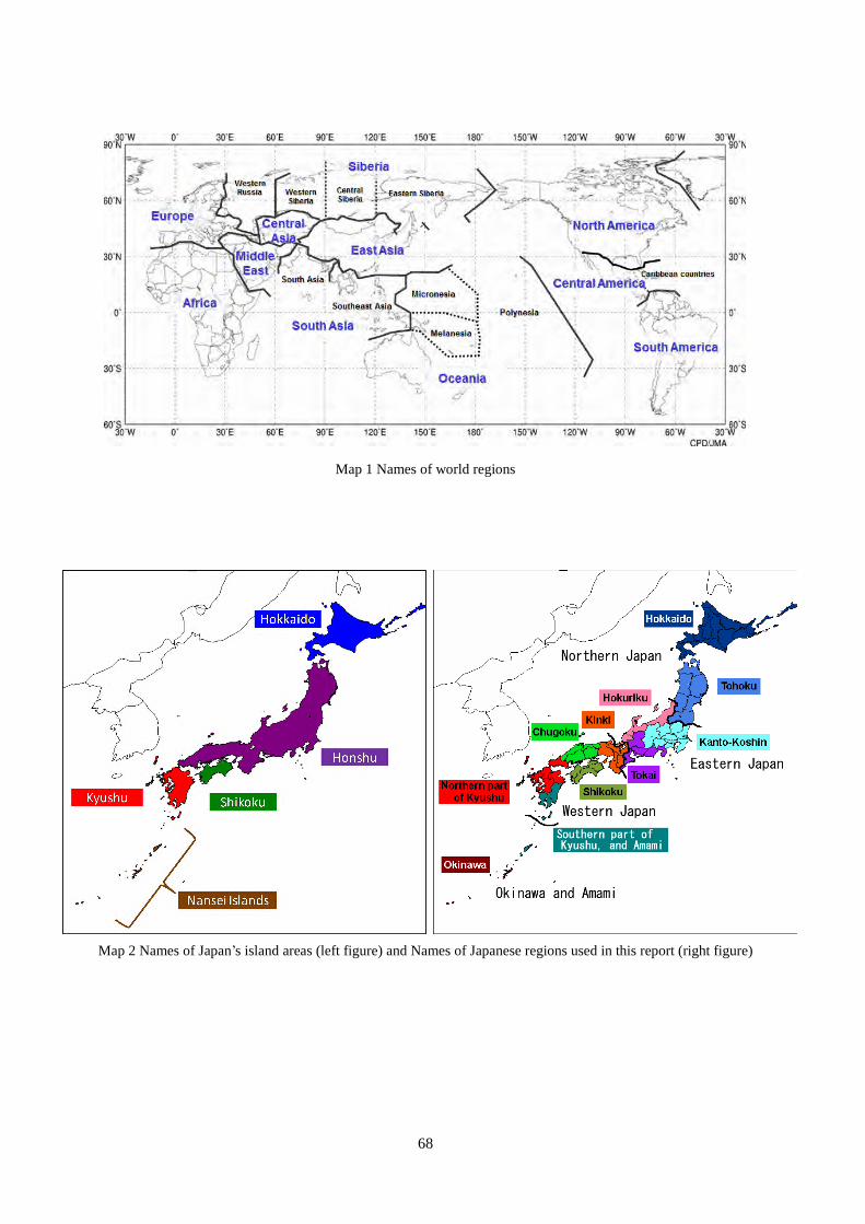
68
Map 1 Names of world regions
Map 2 Names of Japan’s island areas (left figure) and Names of Japanese regions used in this report (right figure)
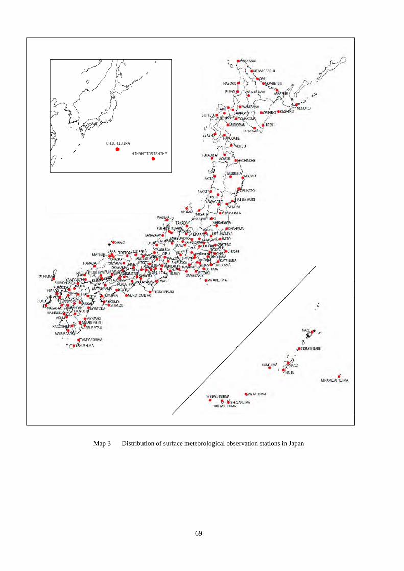
69
Map 3 Distribution of surface meteorological observation stations in Japan
MINAMITORISHIMA CHICHIJIMA
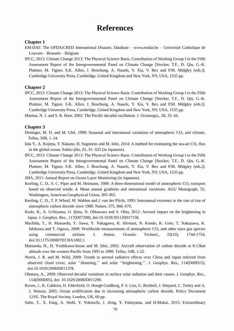
70
References
Chapter 1 EM-DAT: The OFDA/CRED International Disaster, Database – www.emdat.be – Université Catholique de
Louvain – Brussels – Belgium IPCC, 2013: Climate Change 2013: The Physical Science Basis. Contribution of Working Group I to the Fifth
Assessment Report of the Intergovernmental Panel on Climate Change [Stocker, T.F., D. Qin, G.-K. Plattner, M. Tignor, S.K. Allen, J. Boschung, A. Nauels, Y. Xia, V. Bex and P.M. Midgley (eds.)]. Cambridge University Press, Cambridge, United Kingdom and New York, NY, USA, 1535 pp.
Chapter 2 IPCC, 2013: Climate Change 2013: The Physical Science Basis. Contribution of Working Group I to the Fifth
Assessment Report of the Intergovernmental Panel on Climate Change [Stocker, T.F., D. Qin, G.-K. Plattner, M. Tignor, S.K. Allen, J. Boschung, A. Nauels, Y. Xia, V. Bex and P.M. Midgley (eds.)]. Cambridge University Press, Cambridge, United Kingdom and New York, NY, USA, 1535 pp.
Mantua, N. J. and S. R. Hare, 2002: The Pacific decadal oscillation. J. Oceanogra., 58, 35–44. Chapter 3 Dettinger, M. D. and M. Ghil, 1998: Seasonal and interannual variations of atmospheric CO2 and climate.
Tellus, 50B, 1–24. Iida Y., A. Kojima, T. Nakano, H. Sugimoto and M. Ishii, 2014: A method for estimating the sea-air CO2 flux
in the global ocean. Sokko-jiho, 81, S1–S25 (in Japanese). IPCC, 2013: Climate Change 2013: The Physical Science Basis. Contribution of Working Group I to the Fifth
Assessment Report of the Intergovernmental Panel on Climate Change [Stocker, T.F., D. Qin, G.-K. Plattner, M. Tignor, S.K. Allen, J. Boschung, A. Nauels, Y. Xia, V. Bex and P.M. Midgley (eds.)]. Cambridge University Press, Cambridge, United Kingdom and New York, NY, USA, 1535 pp.
JMA, 2011: Annual Report on Ozone Layer Monitoring (in Japanese). Keeling, C. D., S. C. Piper and M. Heimann, 1989: A three-dimensional model of atmospheric CO2 transport
based on observed winds: 4. Mean annual gradients and interannual variations. AGU Monograph, 55, Washington, American Geophysical Union, 305-363.
Keeling, C. D., T. P. Whorf, M. Wahlen and J. van der Plicht, 1995: Interannual extremes in the rate of rise of atmospheric carbon dioxide since 1980. Nature, 375, 666–670.
Kudo, R., A. Uchiyama, O. Ijima, N. Ohkawara and S. Ohta, 2012: Aerosol impact on the brightening in Japan. J. Geophys. Res., 117(D07208), doi:10.1029/2011JD017158.
Machida, T., H. Matsueda, Y. Sawa, Y. Nakagawa, K. Hirotani, N. Kondo, K. Goto, T. Nakazawa, K. Ishikawa and T. Ogawa, 2008: Worldwide measurements of atmospheric CO2 and other trace gas species using commercial airlines. J. Atmos. Oceanic Technol., 25(10), 1744-1754, doi:10.1175/2008JTECHA1082.1.
Matsueda, H., H. Yoshikawa-Inoue and M. Ishii, 2002: Aircraft observation of carbon dioxide at 8-13km altitude over the western Pacific from 1993 to 1999. Tellus, 54B, 1-22.
Norris, J. R. and M. Wild, 2009: Trends in aerosol radiative effects over China and Japan inferred from observed cloud cover, solar ‘‘dimming,’’ and solar ‘‘brightening,’’. J. Geophys. Res., 114(D00D15), doi:10.1029/2008JD011378.
Ohmura, A., 2009: Observed decadal variations in surface solar radiation and their causes. J. Geophys. Res., 114(D00D05), doi: 10.1029/2008JD011290.
Raven, J., K. Caldeira, H. Elderfield, O. Hoegh-Guldberg, P. S. Liss, U. Reisbell, J. Shepard, C. Turley and A. J. Watson, 2005: Ocean acidification due to increasing atmospheric carbon dioxide. Policy Document 12/05. The Royal Society, London, UK, 60 pp.
Saito, T., X. Fang, A. Stohl, Y. Yokouchi, J. Zeng, Y. Fukuyama, and H.Mukai, 2015: Extraordinary
71
halocarbon emissions initiated by the 2011 Tohoku earthquake. Geophys. Res. Lett., 42, doi:10.1002/2014GL062814.
Sawa, Y., T. Machida and H. Matsueda, 2012: Aircraft observation of the seasonal variation in the transport of CO2 in the upper atmosphere. J. Geophys. Res., 117(D05305), doi: 10.1029/2011JDO16933.
Sugimoto, H., N. Hiraishi, T. Midorikawa and M. Ishii, 2012: A method for estimating the sea-air CO2 flux in the Pacific Ocean. Technical Reports of the Meteorological Research Institute, 66, 32pp.
UNEP, 2015: Environmental effects of ozone depletion and its interactions with climate change: 2014 assessment, 236pp.
WCRP, 2010: Summary Report from the Eleventh Baseline Surface Radiation Network (BSRN) Scientific Review andWorkshop. WCRP Informal Report No. 08/2010, 21 pp.
Wild, M., 2009: Global dimming and brightening: A review. J. Geophys. Res., 114(D00D16), doi:10.1029/2008JD011470.
Wild M. and A. Ohmura, 2004: BSRN longwave downward radiation measurements combined with GCMs show promise for greenhouse detection studies, GEWEX news, 14(4), 20pp.
WMO, 2009: Technical Report of Global Analysis Method for Major Greenhouse Gases by the World Data Center for Greenhouse Gases. GAW Report, 184, WMO/TD No.1473.
WMO, 2014: Scientific Assessment of Ozone Depletion: 2014. Global Ozone Research and Monitoring Project-Report, 55, 416 pp.
WMO, 2014: WMO Greenhouse Gas Bulletin No.10. (http://www.wmo.int/pages/prog/arep/gaw/ghg/GHGbulletin.html