Ch15 LMM1 Sample

7/28/2019 Ch15 LMM1 Sample

http://slidepdf.com/reader/full/ch15-lmm1-sample 1/63

andersen-piterbarg-book.com September 9, 2009

S A M P L E

(c) Andersen, Piterbarg 2009

15

The Libor Market Model I

Many of the models considered so far describe the evolution of the yield curvein terms of a small set of Markov state variables. While proper calibration

procedures allow for successful application of such models to the pricing andhedging of a surprising variety of securities, many exotic derivatives requirericher dynamics than what is possible with low-dimensional Markov models.For instance, exotic derivatives may be strongly sensitive to the joint evolutionof multiple points of the yield curve, necessitating the usage of several drivingBrownian motions. Also, most exotic derivatives may not be related in anyobvious way to vanilla European options, making it hard to confidently iden-tify a small, representative set of vanilla securities to which a low-dimensionalMarkovian model can feasibly be calibrated. What is required in such situa-tions is a model sufficiently rich to capture the full correlation structure acrossthe entire yield curve and to allow for volatility calibration to a large enoughset of European options that the volatility characteristics of most exotic se-curities can be considered “spanned” by the calibration. Candidates for sucha model include the multi-factor short-rate models in Chapter 13 and themulti-factor quasi-Gaussian models in Section 14.3. In this chapter, we shallcover an alternative approach to the construction of multi-factor interest ratemodels, the so-called Libor market (LM) model framework. Originally devel-oped in Brace et al. [1996], Jamshidian [1997], and Miltersen et al. [1997],the LM model class enjoys significant popularity with practitioners and is inmany ways easier to grasp than, say, the multi-factor quasi-Gaussian modelsin Chapter 14.

This chapter develops the basic LM model and provides a series of exten-sions to the original log-normal framework in Brace et al. [1996] and Miltersenet al. [1997] in order to better capture observed volatility smiles. To facilitatecalibration of the model, efficient techniques for the pricing of European se-

curities are developed. We provide a detailed discussion of the modeling of forward rate correlations which, along with the pricing formulas for caps andswaptions, serves as the basis for most of the calibration strategies that we pro-ceed to examine. Many of these strategies are generic in nature and apply to




S A M P L E


542 15 The Libor Market Model I

multi-factor models other than the LM class, including the models discussedin Chapters 13 and 14. We wrap up the chapter with a careful discussion of schemes for Monte Carlo simulation of LM models. A number of advancedtopics in LM modeling will be covered in Chapter 16.

15.1 Introduction and Setup

15.1.1 Motivation and Historical Notes

Chapter 5 introduced the HJM framework which, in its most general form,involves multiple driving Brownian motions and an infinite set of state vari-ables (namely the set of instantaneous forward rates). As argued earlier, theHJM framework contains any arbitrage-free interest rate model adapted to afinite set of Brownian motions. Working directly with instantaneous forwardrates is, however, not particularly attractive in applications, for a variety of

reasons. First, instantaneous forward rates are never quoted in the market,nor do they figure directly in the payoff definition of any traded derivativecontract. As discussed in Chapter 6, realistic securities (swaps, caps, futures,etc.) instead involve simply compounded (Libor) rates, effectively represent-ing integrals of instantaneous forwards. The disconnect between market ob-servables and model primitives often makes development of market-consistentpricing expression for simple derivatives cumbersome. Second, an infinite setof instantaneous forward rates can generally1 not be represented exactly on acomputer, but will require discretization into a finite set. Third, prescribingthe form of the volatility function of instantaneous forward rates is subject toa number of technical complications, requiring sub-linear growth to preventexplosions in the forward rate dynamics, which precludes the formulation of a log-normal forward rate model (see Sandmann and Sondermann [1997] and

the discussion in Sections 5.5.3 and 12.1.3).As discovered in Brace et al. [1996], Jamshidian [1997], and Miltersen et al.

[1997], the three complications above can all be addressed simultaneously bysimply writing the model in terms of a non-overlapping set of simply com-pounded Libor rates. Not only do we then conveniently work with a finiteset of directly observable rates that can be represented on a computer, but,as we shall show, an explosion-free log-normal forward rate model also be-comes possible. Despite the change to simply compounded rates, we shouldemphasize that the Libor market model will still be a special case of an HJMmodel, albeit one where we only indirectly specify the volatility function of the instantaneous forward rates.

1As we have seen in earlier chapters, for special choices of the forward ratevolatility we can sometimes identify a finite-dimensional Markovian representationof the forward curve that eliminates the need to store the entire curve. This is notpossible in general, however.




S A M P L E


15.2 LM Dynamics and Measures 543

15.1.2 Tenor Structure

The starting point for our development of the LM model is a fixed tenor structure

0 = T 0 < T 1 < .. . < T N . (15.1)

The intervals τ n = T n+1 − T n, n = 0, . . . , N − 1, would typically be set tobe either 3 or 6 months, corresponding to the accrual period associated withobservable Libor rates. Rather than keeping track of an entire yield curve, atany point in time t we are (for now) focused only on a finite set of zero-couponbonds P (t, T n) for the set of n’s for which T N ≥ T n > t; notice that this setshrinks as t moves forward, becoming empty when t > T N . To formalize this

“roll-off” of zero-coupon bonds in the tenor structure as time progresses, it isoften useful to work with an index function q (t), defined by the relation

T q(t)−1 ≤ t < T q(t). (15.2)

We think of q (t) as representing the tenor structure index of the shortest-dateddiscount bond still alive.On the fixed tenor structure, we proceed to define Libor forward rates

according to the relation (see (5.2))

L(t, T n, T n+1) = Ln(t) =

P (t, T n)

P (t, T n+1)− 1

τ −1n , N − 1 ≥ n ≥ q (t).

We note that when considering a given Libor forward rate Ln(t), we alwaysassume n ≥ q (t) unless stated otherwise. For any T n > t,

P (t, T n) = P (t, T q(t))n−1

i=q(t)

(1 + Li(t)τ i)−1 . (15.3)

Notice that knowledge of Ln(t) for all n ≥ q (t) is generally not sufficient toreconstruct discount bond prices on the entire (remaining) tenor structure;the front “stub” discount bond price P (t, T q(t)) must also be known.

15.2 LM Dynamics and Measures

15.2.1 Setting

In the Libor market model, the set of Libor forwardsLq(t)(t),Lq(t)+1(t), . . . , LN −1(t) constitute the set of state variables for

which we wish to specify dynamics. As a first step, we pick a probabilitymeasure P and assume that those dynamics originate from an m-dimensionalBrownian motion W (t), in the sense that all Libor rates are measurable withrespect to the filtration generated by W (·). Further assuming that the Libor




S A M P L E



rates are square integrable, it follows from the Martingale RepresentationTheorem that, for all n ≥ q (t),

dLn(t) = σn(t)⊤ (µn(t) dt + dW (t)) , (15.4)

where µn and σn are m-dimensional processes, respectively, both adapted tothe filtration generated by W (·). From the Diffusion Invariance Principle (seeSection 2.5) we know that σn(t) is measure invariant, whereas µn(t) is not.

As it turns out, for a given choice of σn in the specification (15.4), itis quite straightforward to work out explicitly the form of µn(t) in variousmartingale measures of practical interest. We turn to this shortly, but let usfirst stress that (15.4) allows us to use a different volatility function σn for eachof the forward rates Ln(t), n = q (t), . . . , N − 1, in the tenor structure. Thisobviously gives us tremendous flexibility in specifying the volatility structureof the forward curve evolution, but in practice will require us to impose quitea bit of additional structure on the model to ensure realism and to avoid anexcess of parameters. We shall return to this topic later in this chapter.

15.2.2 Probability Measures

As shown in Lemma 5.2.3, Ln(t) must be a martingale in the T n+1-forwardmeasure QT n+1, such that, from (15.4),

dLn(t) = σn(t)⊤ dW n+1(t), (15.5)

where W n+1(·) W T n+1(·) is an m-dimensional Brownian motion in QT n+1 .It is to be emphasized that only one specific Libor forward rate — namelyLn — is a martingale in the T n+1-forward measure. To establish dynamics inother probability measures, the following proposition is useful.

Proposition 15.2.1. Let Ln satisfy ( 15.5 ). In measure QT n the process for Ln is

dLn(t) = σn(t)⊤

τ nσn(t)

1 + τ nLn(t)dt + dW n(t)

,

where W n is an m-dimensional Brownian motion in measure QT n.

Proof. From Theorem 2.4.2 we know that the density relating the measuresQT n+1 and QT n is given by

ς (t) = ET n+1t

dQT n

dQT n+1=

P (t, T n)/P (0, T n)P (t, T n+1)/P (0, T n+1)

= (1 + τ nLn(t))P (0, T n+1)

P (0, T n).

Clearly, then,




S A M P L E



dς (t) =P (0, T n+1)

P (0, T n)τ n dLn(t) =

P (0, T n+1)

P (0, T n)τ nσn(t)⊤ dW n+1(t),

or

dς (t)/ς (t) =

τ nσn(t)⊤ dW n+1(t)

1 + τ nLn(t) .

From the Girsanov theorem (Theorem 2.5.1), it follows that the process

dW n(t) = dW n+1(t) − τ nσn(t)

1 + τ nLn(t)dt (15.6)

is a Brownian motion in QT n. The proposition then follows directly from (15.5).⊓⊔

To gain some further intuition for the important result in Proposition15.2.1, let us derive it in less formal fashion. For this, consider the forwarddiscount bond P (t, T n, T n+1) = P (t, T n+1)/P (t, T n) = (1 + τ nLn(t))

−1 . Anapplication of Ito’s lemma to (15.5) shows that

dP (t, T n, T n+1)

= τ 2n (1 + τ nLn(t))−3 σn(t)⊤σn(t) dt − τ n (1 + τ nLn(t))

−2 σn(t)⊤ dW n+1(t)

= τ n (1 + τ nLn(t))−2 σn(t)⊤

τ n (1 + τ nLn(t))

−1 σn(t) dt − dW n+1(t)

.

As P (t, T n, T n+1) must be a martingale in the QT n-measure, it follows that

−dW n(t) = τ n (1 + τ nLn(t))−1 σn(t) dt − dW n+1(t)

is a Brownian motion in QT n , consistent with the result in Proposition 15.2.1.While Proposition 15.2.1 only relates “neighboring” measures QT n+1 and

QT n, it is straightforward to use the proposition iteratively to find the drift of

Ln(t) in any of the probability measures discussed in Section 5.2. Let us givesome examples.

Lemma 15.2.2. Let Ln satisfy ( 15.5 ). Under the terminal measure QT N the process for Ln is

dLn(t) = σn(t)⊤

−N −1

j=n+1

τ jσj(t)

1 + τ jLj(t)dt + dW N (t)

,

where W N is an m-dimensional Brownian motion in measure QT N .

Proof. From (15.6) we know that

dW N (t) = dW N −1(t) + τ N −1σN −1(t)1 + τ N −1LN −1(t)

dt

= dW N −2(t) +τ N −2σN −2(t)

1 + τ N −2LN −2(t)dt +

τ N −1σN −1(t)

1 + τ N −1LN −1(t)dt.




S A M P L E



Continuing this iteration down to W n+1, we get

dW N (t) = dW n+1(t) +N −1

j=n+1

τ jσj(t)

1 + τ jLj(t)dt.

The lemma now follows from (15.5). ⊓⊔Lemma 15.2.3. Let Ln satisfy ( 15.5 ). Under the spot measure QB (see Sec-tion 5.2.3 ) the process for Ln is

dLn(t) = σn(t)⊤

nj=q(t)

τ jσj(t)

1 + τ jLj(t)dt + dW B(t)

, (15.7)

where W B is an m-dimensional Brownian motion in measure QB.

Proof. Recall from Section 5.2.3 that the spot measure is characterized by a

rolling or “jumping” numeraire

B(t) = P

t, T q(t)

q(t)−1n=0

(1 + τ nLn(T n)) . (15.8)

At any time t, the random part of the numeraire is the discount bondP

t, T q(t)

, so effectively we need to establish dynamics in the measure QT q(t) .

Applying the iteration idea shown in the proof of Lemma 15.2.2, we get

dW n+1(t) = dW q(t)(t) +

nj=q(t)

τ jσj(t)

1 + τ jLj(t)dt,

as stated. ⊓⊔The spot and terminal measures are, by far, the most commonly used

probability measures in practice. Occasionally, however, it may be beneficialto use one of the hybrid measures discussed earlier in this book, for instanceif one wishes to enforce that a particular Libor rate Ln(t) be a martingale. Asshown in Section 5.2.4, we could pick as a numeraire the asset price process

P n+1(t) =

P (t, T n+1), t ≤ T n+1,B(t)/B(T n+1), t > T n+1,

(15.9)

where B is the spot numeraire (15.8). Using the same technique as in theproofs of Lemmas 15.2.2 and 15.2.3, it is easily seen that now

dLi(t) =σi(t)⊤ −n

j=i+1τ jσj(t)

1+τ jLj(t)dt + dW n+1(t) , t ≤ T n+1,

σi(t)⊤i

j=q(t)τ jσj(t)

1+τ jLj(t)dt + dW n+1(t)

, t > T n+1,




S A M P L E



whereW n+1(t) is a Brownian motion in the measure induced by the numeraireP n+1(t). Note in particular that Ln(t) is a martingale as desired, and that wehave defined a numeraire which — unlike P (t, T n) — will be alive at any timet.

We should note that an equally valid definition of a hybrid measure willreplace (15.9) with the asset process

P n+1(t) =

B(t), t ≤ T n+1,B(T n+1)P (t, T N )/P (T n+1, T N ), t > T n+1.

(15.10)

This type of numeraire process is often useful in discretization of the LMmodel for simulation purposes; see Section 15.6.1.2 for details.

15.2.3 Link to HJM Analysis

As discussed earlier, the LM model is a special case of the general HJM class

of diffusive interest rate models. To explore this relationship a bit further, werecall that HJM models generally has risk-neutral dynamics of the form

df (t, T ) = σf (t, T )⊤ T

t

σf (t, u) dudt + σf (t, T )⊤ dW (t),

where f (t, T ) is the time t instantaneous forward rate to time T and σf (t, T )is the instantaneous forward rate volatility function. From the results in Chap-ter 5, it follows that dynamics for the forward bond P (t, T n, T n+1) is of theform

dP (t, T n, T n+1)

P (t, T n, T n+1)= O(dt) −

σP (t, T n+1)⊤ − σP (t, T n)⊤

dW (t),

where O(dt) is a drift term and

σP (t, T ) =

T

t

σf (t, u) du.

By definition Ln(t) = τ −1n (P (t, T n, T n+1)−1 − 1), such that

dLn(t) = O(dt) + τ −1n (1 + τ nLn(t))

T n+1

T n

σf (t, u)⊤ dudW (t).

By the Diffusion Invariance Principle (see Section 2.5), it follows from (15.5)that the LM model volatility σn(t) is related to the HJM instantaneous for-

ward volatility function σf (t, T ) by

σn(t) = τ −1n (1 + τ nLn(t))

T n+1

T n

σf (t, u) du. (15.11)




S A M P L E



Note that, as expected, σn(t) → σf (t, T n) as τ n → 0.It should be obvious from (15.11) that a complete specification of σf (t, T )

uniquely determines the LM volatility σn(t) for all t and all n. On the otherhand, specification of σn(t) for all t and all n does not allow us to imply a

unique HJM forward volatility function σf (t, T ) — all we are specifying isessentially a strip of contiguous integrals of this function in the T -direction.This is hardly surprising, inasmuch as the LM model only concerns itself witha finite set of discrete interest rate forwards and as such cannot be expectedto uniquely characterize the behaviors of instantaneous forward rates andtheir volatilities. Along the same lines, we note that the LM model does notuniquely specify the behavior of the short rate r(t) = f (t, t); as a consequence,the rolling money-market account β (t) and the risk-neutral measure are notnatural constructions in the LM model2. Section 16.3 discusses these issues inmore details.

15.2.4 Separable Deterministic Volatility Function

So far, our discussion of the LM model has been generic, with little structureimposed on the N − 1 volatility functions σn(t), n = 1, 2, . . . , N − 1. To builda workable model, however, we need to be more specific about our choice of σn(t). A common prescription of σn(t) takes the form

σn(t) = λn(t)ϕ (Ln(t)) , (15.12)

where λn(t) is a bounded vector-valued deterministic function and ϕ : R → R

is a time-homogeneous local volatility function. This specification is concep-tually very similar to the local volatility models in Chapter 8, although hereσn(t) is vector-valued and the model involves simultaneous modeling of mul-tiple state variables (the N − 1 Libor forwards).

At this point, the reader may reasonably ask whether the choice (15.12)in fact leads to a system of SDEs for the various Libor forward rates thatis “reasonable”, in the sense of existence and uniqueness of solutions. Whilewe here shall not pay much attention to such technical regularity issues, itshould be obvious that not all functions ϕ can be allowed. One relevant resultis given below.

Proposition 15.2.4. Assume that ( 15.12 ) holds with ϕ(0 ) = 0 and that Ln(0) ≥ 0 for all n. Also assume that ϕ is locally Lipschitz continuous and satisfies the growth condition

ϕ(x)2 ≤ C

1 + x2

, x > 0,

where C is some positive constant. Then non-explosive, pathwise unique solu-

tions of the no-arbitrage SDEs for Ln(t), q (t) ≤ n ≤ N − 1, exist under all measures QT i , q (t) ≤ i ≤ N . If Ln(0) > 0, then Ln(t) stays positive at all t.

2In fact, as discussed in Jamshidian [1997], one does not need to assume that ashort rate process exist when constructing an LM model.




S A M P L E



Proof. (Sketch) Due to the recursive relationship between measures, it sufficesto consider the system of SDEs (15.7) under the spot measure QB:

dLn(t) = ϕ (Ln(t)) λn(t)⊤ µn(t) dt + dW B(t) , (15.13)

µn(t) =n

j=q(t)

τ jϕ (Lj(t)) λj(t)

1 + τ jLj(t). (15.14)

Under our assumptions, it is easy to see that each term in the sum for µn islocally Lipschitz continuous and bounded. The growth condition on ϕ in turnensures that the product ϕ (Ln(t)) λn(t)⊤µn(t) is also locally Lipschitz con-tinuous and, due to the boundedness of µn, satisfies a linear growth condition.Existence and uniqueness now follows from Theorem 2.6.1. The result that 0is a non-accessible boundary for the forward rates if started above 0 followsfrom standard speed-scale boundary classification results; see Andersen andAndreasen [2000b] for the details. ⊓⊔

Some standard parameterizations of ϕ are shown in Table 15.1. Of those,only the log-normal specification and the LCEV specification directly satisfythe criteria in Proposition 15.2.4. The CEV specification violates Lipschitzcontinuity at x = 0, and as a result uniqueness of the SDE fails. As shownin Andersen and Andreasen [2000b], we restore uniqueness by specifying thatforward rates are absorbed at the origin (see also Section 8.2.3). As for thedisplaced diffusion specification ϕ(x) = ax+b, we here violate the assumptionthat ϕ(0) = 0, and as a result we cannot always guarantee that forward ratesstay positive. Also, to prevent explosion of the forward rate drifts, we need toimpose additional restrictions to prevent terms of the form 1+τ nLn(t) from be-coming zero. As displaced diffusions are of considerable practical importance,we list the relevant restrictions in Lemma 15.2.5 below.

Name ϕ(x)

Log-normal x

CEV xp, 0 < p < 1LCEV x min

εp−1, xp−1

, 0 < p < 1, ε > 0

Displaced log-normal bx + a, b > 0, a = 0

Table 15.1. Common DVF Specifications

Lemma 15.2.5. Consider a local volatility Libor market model with local volatility function ϕ(x) = bx + a, where b > 0 and a = 0. Assume that

bLn(0)+ a > 0 and a/b < τ −1n for all n = 1, 2, . . . , N − 1. Then non-explosive,

pathwise unique solutions of the no-arbitrage SDEs for Ln(t), q (t) ≤ n ≤ N −1,exist under all measures QT i , q (t) ≤ i ≤ N . All Ln(t) are bounded from below by −a/b.




S A M P L E



Proof. Define H n(t) = bLn(t) + a. By Ito’s lemma, we have

dH n(t) = b dLn(t) = bH n(t)λn(t)⊤

µn(t) dt + dW B(t)

,

µn(t) =

nj=q(t)

τ jH j(t)λj(t)

1 + τ j (H j(t) − a) /b .

From the assumptions of the lemma, we have H n(0) > 0 for all n, allowingus to apply the result of Proposition 15.2.4 to H n(t), provided that we canguarantee that µn(t) is bounded for all positive H j , j = q (t), . . . , n. Thisfollows from 1 − τ ja/b > 0 or a/b < τ −1

j . ⊓⊔We emphasize that the requirement a/b < τ −1

n implies that only in thelimit of τ j → 0 — where the discrete Libor forward rates become instanta-neous forward rates — will a pure Gaussian LM model specification (b = 0)be meaningful; such a model was outlined in Section 5.5.1. On the flip-side,according to Proposition 15.2.4, a finite-sized value of τ j ensures that a well-behaved log-normal forward rate model exists, something that we saw earlier

(Section 12.1.3) was not the case for models based on instantaneous forwardrates. The existence of log-normal forward rate dynamics in the LM settingwas, in fact, a major driving force behind the development and populariza-tion of the LM framework, and all early examples of LM models (see Braceet al. [1996], Jamshidian [1997], and Miltersen et al. [1997]) were exclusivelylog-normal.

We recall from earlier chapters that it is often convenient to specify dis-placed diffusion models as ϕ(Ln(t)) = (1 − b)Ln(0) + bLn(t), in which casethe constant a in Lemma 15.2.5 is different from one Libor rate to the next.In this case, we must require

(1 − b)/b < (Ln(0)τ n)−1, n = 1, . . . , N − 1.

As Ln(0)τ n is typically in the magnitude of a few percent, the regularityrequirement on b in (15.2.4) is not particularly restrictive.

15.2.5 Stochastic Volatility

As discussed earlier in this book, to ensure that the evolution of the volatilitysmile is reasonably stationary, it is best if the skew function ϕ in (15.14) is(close to) monotonic in its argument. Typically we are interested in specifica-tions where ϕ(x)/x is downward-sloping, to establish the standard behaviorof interest rate implied volatilities tending to increase as interest rates decline.In reality, however, markets often exhibit non-monotonic volatility smiles or

“smirks” with high-struck options trading at implied volatilities above the at-

the-money levels. An increasingly popular mechanism to capture such behav-ior in LM models is through the introduction of stochastic volatility. We havealready encountered stochastic volatility models in Chapters 9, 10 and, in thecontext of term structure models, in Sections 14.2 and 14.3; we now discuss




S A M P L E



how to extend the notion of stochastic volatility models to the simultaneousmodeling of multiple Libor forward rates.

As our starting point, we take the process (15.14), preferably equippedwith a ϕ that generates either a flat or monotonically downward-sloping volatil-

ity skew, but allow the term on the Brownian motion to be scaled by a stochas-tic process. Specifically, we introduce a mean-reverting scalar process z, withdynamics of the form

dz(t) = θ (z0 − z(t)) dt + ηψ (z(t)) dZ (t), z(0) = z0, (15.15)

where θ, z0, and η are positive constants, Z is a Brownian motion under thespot measure QB, and ψ : R+ → R+ is a well-behaved function. We imposethat (15.15) will not generate negative values of z, which requires ψ(0) = 0.We will interpret the process in (15.15) as the (scaled) variance process forour forward rate diffusions, in the sense that the square root of z will be usedas a stochastic, multiplicative shift of the diffusion term in (15.14). That is,our forward rate processes in QB are, for all n ≥ q (t),

dLn(t) = z(t)ϕ (Ln(t)) λn(t)⊤ z(t)µn(t) dt + dW B(t) , (15.16)

µn(t) =n

j=q(t)

τ jϕ (Lj(t)) λj(t)

1 + τ jLj(t),

where z(t) satisfies (15.15). This construction naturally follows the specifica-tion of vanilla stochastic volatility models in Chapter 9, and the specificationof stochastic volatility quasi-Gaussian models in Chapter 14. As we discussedpreviously, it is often natural to scale the process for z such that z(0) = z0 = 1.

Let us make two important comments about (15.16). First, we emphasizethat a single common factor

√ z simultaneously scales all forward rate volatil-

ities; movements in volatilities are therefore perfectly correlated across the

various forward rates. In effect, our model corresponds only to the first princi-pal component of the movements of the instantaneous forward rate volatilities.This is a common assumption that provides good balance between realism andparsimony, and we concentrate mostly on this case — although we do relax itlater in the book, in Chapter 16. Second, we note that the clean form of thez-process (15.15) in the measure QB generally does not carry over to otherprobability measures, as we would expect from Proposition 9.3.9. To statethe relevant result, let Z (t), W (t) denote the quadratic covariation betweenZ (t) and the m components of W (t) (recall the definition of covariation inRemark 2.1.7). We then have

Lemma 15.2.6. Let dynamics for z(t) in the measure QB be as in ( 15.15 ).Then the SDE for z(t) in measure QT n+1 , n

≥q (t)

−1, is

dz(t) = θ (z0 − z(t)) dt + ηψ (z(t))

×−

z(t)µn(t)⊤

dZ (t), dW B(t)

+ dZ n+1(t)

, (15.17)




S A M P L E



where µn(t) is given in ( 15.16 ) and Z n+1 is a Brownian motion in measure QT n+1 .

Proof. From earlier results, we have

dW n+1(t) = z(t)µn(t) dt + dW B(t).

Let us denotea(t) =

dZ (t), dW B(t)

/dt,

so that we can write

dZ (t) = a(t)⊤ dW B(t) +

1 − a(t)2 dW (t),

where W is a scalar Brownian motion independent of W B. In the measureQT n+1 , we then have

dZ (t) = a(t)⊤ dW n+1(t)

− z(t)µn(t) dt + 1 − a(t)

2 dW (t)

= dZ n+1(t) − a(t)⊤ z(t)µn(t) dt,

and the result follows. ⊓⊔The process (15.17) is awkward to deal with, due to presence of the drift

term µn(t)⊤

dZ (t), dW B(t)

which will, in general, depend on the state of theLibor forward rates at time t. For tractability, on the other hand, we would likefor the z-process to only depend on z itself. To achieve this, and to generallysimplify measure shifts in the model, we make the following assumption3 about(15.15)–(15.16):

Assumption 15.2.7. The Brownian motion Z (t) of the variance process z(t)is independent of the vector-valued Brownian motion W B(t).

We have already encountered the same assumption in the context of stochastic volatility quasi-Gaussian models, see Section 14.2.1, where we alsohave a discussion of the implications of such a restriction.

The diffusion coefficient of the variance process, the function ψ, is tradi-tionally chosen to be of power form, ψ(x) = xα, α > 0. While it probablymakes sense to keep the function monotone, the power specification is proba-bly a nod to tradition rather than anything else. Nevertheless, some particularchoices lead to analytically tractable specifications, as we saw in Chapter 9;for that reason, α = 1/2 (the Heston model) is popular.

Remark 15.2.8. Going forward we shall often use the stochastic volatility (SV)model in this section as a benchmark for theoretical and numerical work. As

the stochastic volatility model reduces to the local volatility model in Section15.2.4 when z(t) is constant, all results for the SV model will carry over tothe DVF setting.

3We briefly return to the general case in Section 16.6.




S A M P L E


15.3 Correlation 553

15.2.6 Time-Dependence in Model Parameters

In the models we outlined in Sections 15.2.4 and 15.2.5, the main role of thevector-valued function of time λn(t) was to establish a term structure “spine”

of at-the-money option volatilities. To build volatility smiles around this spine,we further introduced a universal skew-function ϕ, possibly combined witha stochastic volatility scale z(t) with time-independent process parameters.In practice, this typically gives us a handful of free parameters with whichwe can attempt to match the market-observed term structures of volatilitysmiles for various cap and swaption tenors. As it turns out, a surprisinglygood fit to market skew data can, in fact, often be achieved with the modelsof Sections 15.2.4 and 15.2.5. For a truly precise fit to volatility skews acrossall maturities and swaption tenors, it may, however, be necessary to allowfor time-dependence in both the dynamics of z(t) and, more importantly, theskew function ϕ. The resulting model is conceptually similar to the modelin Section 15.2.5, but involves a number of technical intricacies that draw

heavily on the material presented in Chapter 10. To avoid cluttering this firstchapter on LM model with technical detail, we relegate the treatment of thetime-dependent case to the next chapter on advanced topics in LM modeling.

15.3 Correlation

In a one-factor model for interest rates — such as the ones presented in Chap-ters 11 and 12 — all points on the forward curve always move in the samedirection. While this type of forward curve move indeed is the most commonlyobserved type of shift to the curve, “rotational steepenings” and the formationof “humps” may also take place, as may other more complex types of curveperturbations. The empirical presence of such non-trivial curve movements is

an indication of the fact that various points on the forward curve do not moveco-monotonically with each other, i.e. they are imperfectly correlated. A keycharacteristic of the LM model is the consistent use of vector-valued Brownianmotion drivers, of dimension m, which gives us control over the instantaneouscorrelation between various points on the forward curve.

Proposition 15.3.1. The correlation between forward rate increments dLk(t)and dLj(t) in the SV-model ( 15.16 ) is

Corr(dLk(t), dLj(t)) =λk(t)⊤λj(t)

λk(t) λj(t) .

Proof. Using the covariance notation of Remark 2.1.7, we have, for any j andk,

dLk(t), Lj(t) = z(t)ϕ (Lk(t)) ϕ (Lj(t)) λk(t)⊤λj(t) dt.

Using this in the definition of the correlation,




S A M P L E



Corr(dLk(t), dLj(t)) =dLk(t), dLj(t) dLk(t)dLj(t) ,

gives the result of the proposition.

⊓⊔A trivial corollary of Proposition 15.3.1 is the fact thatCorr(dLk(t), dLj(t)) = 1 always when m = 1, i.e. when we only haveone Brownian motion. As we add more Brownian motions, our abilityto capture increasingly complicated correlation structures progressivelyimproves (in a sense that we shall examine further shortly), but at a cost of increasing the model complexity and, ultimately, computational effort. Tomake rational decisions about the choice of model dimension m, let us turnto the empirical data.

15.3.1 Empirical Principal Components Analysis

For some fixed value of τ (e.g. 0.25 or 0.5) define “sliding” forward rates4 l

with tenor x as l(t, x) = L(t, t + x, t + x + τ ).

For a given set of tenors x1, . . . , xN x and a given set of calendar timest0, t1, . . . , tN t , we use market observations5 to set up the N x × N t observa-tion matrix O with elements

Oi,j =l(tj , xi) − l(tj−1, xi)√

tj − tj−1, i = 1, . . . , N x, j = 1, . . . , N t.

Notice the normalization with√

tj − tj−1 which annualizes the variance of theobserved forward rate increments. Also note that we use absolute incrementsin forward rates here. This is arbitrary — we could have used, say, relativeincreases as well, if we felt that rates were more log-normal than Gaussian.

For small sampling periods, the precise choice is of little importance.Assuming time-homogeneity and ignoring small drift terms, the data col-

lected above will imply a sample N x × N x variance-covariance matrix equalto

C =OO⊤

N t.

For our LM model to conform to empirical data, we need to use a suffi-ciently high number m of Brownian motions to closely replicate this variance-covariance matrix. A formal analysis of what value of m will suffice can pro-ceed with the tools of principal components analysis (PCA), as established inSection 4.1.3.

4The use of sliding forward rates, i.e. forward rates with a fixed time to maturityrather than a fixed time of maturity, is often known as the Musiela parameterization .

5For each date in the time grid tj we thus construct the forward curve frommarket observable swaps, futures, and deposits, using techniques such as those inChapter 7.




S A M P L E



15.3.1.1 Example: USD Forward Rates

To give a concrete example of a PCA run, we set N x = 9 and use tenorsof (x1, . . . , x9) = (0.5, 1, 2, 3, 5, 7, 10, 15, 20) years. We fix τ = 0.5 (i.e., all

forwards are 6-months discrete rates) and use 4 years of weekly data from theUSD market, spanning January 2003 to January 2007, for a total of N t = 203curve observations. The eigenvalues of the matrix C are listed in Table 15.2,along with the percentage of variance that is explained by using only the firstm principal components.

m 1 2 3 4 5 6 7 8 9

Eigenvalue 7.0 0.94 0.29 0.064 0.053 0.029 0.016 0.0091 0.0070% Variance 83.3 9 4.5 9 7.9 98.7 99.3 99.6 99.8 99.9 100

Table 15.2. PCA for USD Rates. All eigenvalues are scaled up by 104.

As we see from the table, the first principal component explains about83% of the observed variance, and the first three together explain nearly 98%.This pattern carries over to most major currencies, and in many applicationswe would consequently expect that using m = 3 or m = 4 Brownian motionsin a LM model would adequately capture the empirical covariation of thepoints on the forward curve. An exception to this rule-of-thumb occurs whena particular derivative security depends strongly on the correlation betweenforward rates with tenors that are close to each other; in this case, as we shallsee in Section 15.3.4, a high number of principal components is required toprovide for sufficient decoupling of nearby forwards.

The eigenvectors corresponding to the largest three eigenvectors in Table

15.2 are shown in the Figure 15.1; the figure gives us a reasonable idea aboutwhat the (suitably scaled) first three elements of the λk(t) vectors should looklike as functions of T k − t. Loosely speaking, the first principal componentcan be interpreted as a near-parallel shift of the forward curve, whereas thesecond and third principal components correspond to forward curve twistsand bends, respectively.

15.3.2 Correlation Estimation and Smoothing

Empirical estimates for forward rate correlations can proceed along the linesof Section 15.3.1. Specifically, if we introduce the diagonal matrix

c C 1,1 0 · · · 00 C 2,2 · · · 0

...... · · · 0

0 0 · · · C N x,N x

,




S A M P L E



Fig. 15.1. Eigenvectors

-0.6

-0.4

-0.2

0

0.2

0.4

0.6

0.8

0 5 10 15 20

Forward Rate Maturity (Years)

First Eigenvector

Second EigenvectorThird Eigenvector

Notes: Eigenvectors for the largest three eigenvalues in Table 15.2.

then the empirical N x × N x forward rate correlation matrix R becomes

R = c−1Cc−1.

Element Ri,j of R provides a sample estimate of the instantaneous correlationbetween increments in l(t, xi) and l(t, xi), under the assumption that thiscorrelation is time-homogeneous.

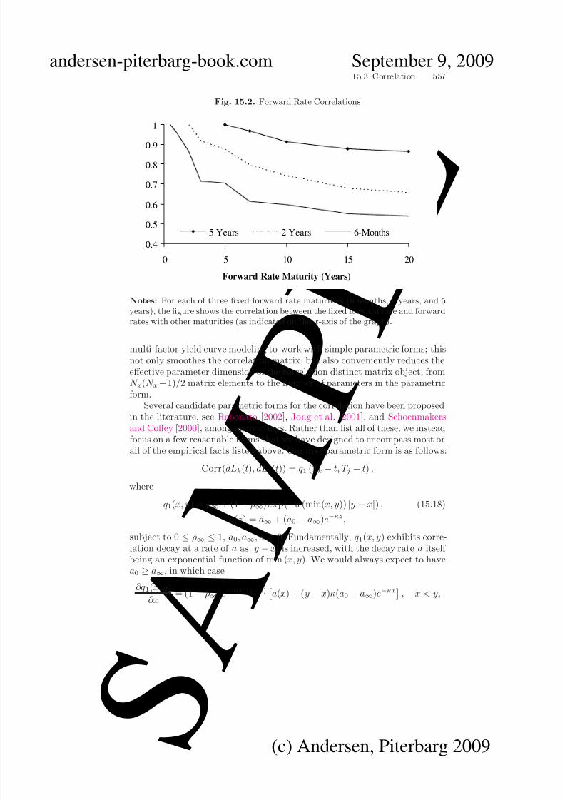
The matrix R is often relatively noisy, partially as a reflection of the factthat correlations are well-known to be quite variable over time, and partiallyas a reflection of the fact that the empirical correlation estimator has ratherpoor sample properties with large confidence bounds (see Johnson et al. [1995]for details). Nevertheless, a few stylistic facts can be gleaned from the data.In Figure 15.2, we have graphed a few slices of the correlation matrix for theUSD data in Section 15.3.1.1.

To make a few qualitative observations about Figure 15.2, we notice thatcorrelations between forward rates l(·, xk) and l(·, xj) generally decline in|xk − xj |; this decline appears near-exponential for xk and xj close to eachother, but with a near-flat asymptote for large |xk − xj |. It appears that therate of the correlation decay and the level of the asymptote depend not only|xk − xj |, but also on min (xk, xj). Specifically, the decay rate decreases withmin(xk, xj), and the asymptote level increases with min (xk , xj).

In practice, unaltered empirical correlation matrices are typically too noisyfor comfort, and might contain non-intuitive entries (e.g., correlation betweena 10-year forward and a 2-year forward might come out higher than betweena 10-year forward and a 5-year forward). As such, it is common practice in




S A M P L E



Fig. 15.2. Forward Rate Correlations

0.4

0.5

0.6

0.7

0.8

0.9

1

0 5 10 15 20

Forward Rate Maturity (Years)

5 Years 2 Years 6-Months

Notes: For each of three fixed forward rate maturities (6 months, 2 years, and 5years), the figure shows the correlation between the fixed forward rate and forwardrates with other maturities (as indicated on the x-axis of the graph).

multi-factor yield curve modeling to work with simple parametric forms; thisnot only smoothes the correlation matrix, but also conveniently reduces theeffective parameter dimension of the correlation distinct matrix object, fromN x(N x −1)/2 matrix elements to the number of parameters in the parametricform.

Several candidate parametric forms for the correlation have been proposed

in the literature, see Rebonato [2002], Jong et al. [2001], and Schoenmakersand Coffey [2000], among many others. Rather than list all of these, we insteadfocus on a few reasonable forms that we have designed to encompass most orall of the empirical facts listed above. Our first parametric form is as follows:

Corr(dLk(t), dLj(t)) = q 1 (T k − t, T j − t) ,

where

q 1(x, y) = ρ∞ + (1 − ρ∞)exp(−a (min(x, y)) |y − x|) , (15.18)

a(z) = a∞ + (a0 − a∞)e−κz,

subject to 0 ≤ ρ∞ ≤ 1, a0, a∞, κ ≥ 0. Fundamentally, q 1(x, y) exhibits corre-lation decay at a rate of a as |y − x| is increased, with the decay rate a itself

being an exponential function of min (x, y). We would always expect to havea0 ≥ a∞, in which case

∂q 1(x, y)

∂x= (1 − ρ∞)e−a(x)(y−x)

a(x) + (y − x)κ(a0 − a∞)e−κx

, x < y,




S A M P L E



is non-negative, as one would expect.Variations on (15.18) are abundant in the literature — the case a0 = a∞

is particularly popular — and q 1 generally has sufficient degrees of freedom toprovide a reasonable fit to empirical data. One immediate issue, however, is a

lack of control of the asymptotic correlation level at |x − y| → ∞ which, as weargued above, is typically not independent of x and y. As the empirical datasuggests that ρ∞ tends to increase with min (x, y), we introduce yet anotherdecaying function

ρ∞(z) = b∞ + (b0 − b∞)e−αz, (15.19)

and extend q 1 to the “triple-decaying” form

q 2(x, y) = ρ∞ (min(x, y)) + (1 − ρ∞ (min(x, y)))exp(−a (min(x, y)) |y − x|)(15.20)

with a(z) is given in (15.18), and where 0 ≤ b0, b∞ ≤ 1, α ≥ 0. Empirical datasuggests that normally b0 ≤ b∞, in which case we have

∂q 2(x, y)∂x

= −α(b0 − b∞)e−αx 1 − e−a(x)(y−x)+ (1 − ρ∞(x)) e−a(x)(y−x) × a(x) + (y − x)κ(a0 − a∞)e−κx

, x < y,

which remains non-negative if b0 ≤ b∞ and a0 ≥ a∞.In a typical application, the four parameters of q 1 and the six parameters of

q 2 are found by least-squares optimization against an empirical correlation ma-trix. Any standard optimization algorithm, such as the Levenberg-Marquardtalgorithm in Press et al. [1992], can be used for this purpose. Some parametersare here subject to simple box-style constraints (e.g. ρ∞ ∈ [0, 1]) which posesno particular problems for most commercial optimizers. In any case, we canalways use functional mappings to rewrite our optimization problem in terms

of variables with unbounded domains. For instance, for form q 1, we can set

ρ∞ =1

2+

arctan(u)

π, u ∈ (−∞, ∞),

and optimize on the variable u instead of ρ∞. Occasionally, we may sometimeswish to optimize correlation parameters against more market-driven targetsthan empirical correlation matrices; see Section 15.5.9 for details on this.

15.3.2.1 Example: Fit to USD data

Let R be the 10 × 10 empirical correlation matrix generated from the datain Section 15.3.1.1, and let R2(ξ ), ξ ≡ (a0, a∞, κ , b0, b∞, α)

⊤, be the 10 × 10

correlation matrix generated from the form q 2, when using the 10 specificforward tenors in 15.3.1.1. To determine the optimal parameter vector ξ ∗, weminimize an unweighted Frobenius (least-squares) matrix norm, subject to anon-negativity constraint




S A M P L E



ξ ∗ = argminξ

tr

(R − R2(ξ )) (R − R2(ξ ))⊤

, subject to ξ ≥ 0.

The resulting fit is summarized in Table 15.3; Figure 15.3 in Section 15.3.4.1contains a 3D plot of the correlation matrix R2(ξ ∗).

a0 a∞ κ b0 b∞ α

0.312 0.157 0.264 0.490 0.946 0.325

Table 15.3. Best-Fit Parameters for q 2 in USD Market

The value of the Frobenius norm at ξ ∗ was 0.070, which translates intoan average absolute correlation error (excluding diagonal elements) of around2%. If we use the four parameter form q 1 instead of q 2 in the optimizationexercise, the Frobenius norm at the optimum increases to 0.164. As we would

expect from Figure 15.2, allowing correlation asymptotes to increase in tenorsthus adds significant explanatory power to the parametric form.

15.3.3 Negative Eigenvalues

While some functional forms are designed to always return valid correlationmatrices (the function in Schoenmakers and Coffey [2000] being one suchexample), many popular forms — including our q 1 and q 2 above — can, whenstressed, generate matrices R that fail to be positive definite. While this rarelyhappens in real applications, it is not inconceivable that on occasion one ormore eigenvalues of R may turn out to be negative, requiring us to somehow

“repair” the matrix. A similar problem can also arise due to rounding errors

when working with large empirical correlation matrices.Formally, when faced with an R matrix that is not positive definite, wewould ideally like to replace it with a modified matrix R∗ which i) is a validcorrelation matrix; and ii) is as close as possible to R, in the sense of somematrix norm. The problem of locating R∗ then involves computing the norm

{R − X : X is a correlation matrix}and setting R∗ equal to the matrix X that minimizes this distance. If · isa weighted Frobenius norm, numerical algorithms for the computation of R∗

have recently emerged, see Higham [2002] for a review and a clean approach.If the negative eigenvalues are small in absolute magnitude (which is often

the case in practice), it is often reasonable to abandon a full-blown optimiza-

tion algorithm in favor of a more heuristic approach where we simply raise alloffending negative eigenvalues to some positive cut-off value; we present oneobvious algorithm below.

As a starting point, we write




S A M P L E



R = EΛE ⊤,

where Λ is a diagonal matrix of eigenvalues, and E is a matrix with theeigenvectors of R in its column. Let Λ∗ be the diagonal matrix with all-positive

entriesΛ∗ii = max(ǫ, Λii), i = 1, . . . , N x,

for some small cut-off value ǫ > 0. Then set

C ∗ = EΛ∗E ⊤,

which we interpret as a covariance matrix, i.e. of the form

C ∗ = c∗R∗c∗

where c∗ is a diagonal matrix with elements c∗ii =

C ∗ii and R∗ is the valid,positive definite correlation matrix we seek. R∗ is then computed as

R∗ = (c∗)−1C ∗(c∗)−1. (15.21)

We emphasize that R∗ as defined in (15.21) will have 1’s in its diagonal,whereas C ∗ will not. Both C ∗ and R∗ are, by construction, positive definite.

15.3.4 Correlation PCA

We now turn to a problem that arises in certain important applications, suchas the calibration procedure we shall discuss in Section 15.5. Consider a p-dimensional Gaussian variable Y , where all elements of Y have zero meanand unit variance. Let Y have a positive definite correlation matrix R, givenby

R = E Y Y ⊤ .

Consider now writing, as an approximation,

Y ≈ DX (15.22)

where X is an m-dimensional vector of independent standard Gaussian vari-ables, m < p, and D is a p×m-dimensional matrix. We wish to strictly enforcethat DX remains a vector of variables with zero means and unit variances,thereby ensuring that the matrix DD⊤ has the interpretation of a valid cor-relation matrix. In particular, we require that the diagonal of DD⊤ is oneeverywhere.

Let v(D) be the p-dimensional vector of the diagonal elements of DD⊤, i.e.

vi = DD

⊤ii, i = 1, . . . , p. Working as before with an unweighted

6

Frobeniusnorm, we set

6The introduction of user-specified weights into this norm is a straightforwardextension.




S A M P L E



h(D; R) = tr

R − DD⊤

R − DD⊤⊤

, (15.23)

and define the optimal choice of D, denoted D∗, as

D∗ = argminDh(D; R), subject to v(D) = 1, (15.24)

where 1 is a p-dimensional vector of 1’s.

Proposition 15.3.2. Let µ be a p-dimensional vector, and let Dµ be given as the unconstrained optimum

Dµ = argminDh(D; R + diag(µ)),

with h given in ( 15.23 ). Define D∗ as in ( 15.24) and let µ∗ be the solution to

v(Dµ) − 1 = 0.

Then D∗ = Dµ∗ .

Proof. We only provide a sketch of the proof; for more details, see Zhang andWu [2003]. First, we introduce the Lagrangian

ℑ (D, µ) = h(D; R) − 2µ⊤ (v(D) − 1) .

(The factor 2 on µ⊤ simplifies results). Standard matrix calculus shows that

dℑdD

=

dℑ

dDi,j

= −4RD + 4DD⊤D.

Setting the derivatives of the Lagrangian ℑ with respect to D and µ to zeroyields, after a little rearrangement,

− (R + diag(µ)) D + DD⊤D = 0, v(D) = 1.

The first of these conditions identifies the optimum as minimizing the (uncon-strained) optimization norm h(D; R + diag(µ)). ⊓⊔Remark 15.3.3. For any fixed value of µ, Dµ can be computed easily by stan-dard PCA methods provided we interpret R+diag(µ) as the target covariancematrix.

With Proposition 15.3.2, determination of D∗ is reduced to solving the p-dimensional root-search problem v (Dµ)−1 = 0 for µ. Many standard methodswill suffice; for instance, one can use straightforward secant search methodssuch as the Broyden algorithm in [Press et al., 1992, p. 389].

As is the case for ordinary PCA approximations of covariance matrices,the “correlation PCA” algorithm outlined so far will return a correlation ma-trix approximation D∗(D∗)⊤ that has reduced rank (from p down to m), aconsequence of the PCA steps taken in estimating Dµ.




S A M P L E



Computation of optimal rank-reduced correlation approximations is a rel-atively well-understood problems, and we should note the existence of sev-eral recent alternatives to the basic algorithm we outline here. A survey canbe found in Pietersz and Groenen [2004] where an algorithm based on ma-

jorization is developed7. We should also note that certain heuristic (and non-optimal) methods have appeared in the literature, some of which are closelyrelated to the simple algorithm we outlined in Section 15.3.3 for repair of correlation matrices. We briefly outline one such approach below (in Section15.3.4.2), but first we consider a numerical example.

15.3.4.1 Example: USD Data

We here consider performing a correlation PCA analysis the correlation matrixR generated from our best-fit form q 2 in Section 15.3.2.1. The 3D plots inFigure 15.3 below show the correlation fit we get with a rank 3 correlationmatrix.

Fig. 15.3. Forward Rate Correlation Matrix in USD

14

710 13 16

19

147

1013

1619 0.4

0.6

0.8

1

14

710

13 1619

147

1013

1619

0.4

0.6

0.8

1

Notes: The right-hand panel shows the correlation matrix R for form q 2 calibratedto USD data. The left-hand panel shows the best-fitting rank-3 correlation matrix,computed by the algorithm in Proposition 15.3.2. In both graphs, the x- and y-axesrepresent the Libor forward rate maturity in years.

Looking at Figure 15.3, the effect of rank-reduction is, loosely, that theexponential decay of our original matrix R has been replaced with a “sigmoid”shape (to paraphrase Riccardo Rebonato) that is substantially too high close

7In our experience, the majorization method in Pietersz and Groenen [2004] isfaster than the method in Proposition 15.3.2 but, contrary to claims in Pieterszand Groenen [2004], less robust, particularly for very large and irregular correlationmatrices.




S A M P L E



to the matrix diagonal. As the rank of the approximating correlation matrixis increased, the sigmoid shape is — often rather slowly — pulled towards ex-ponential shape of the full-rank data. Intuitively, we should not be surprisedat this result: with the rank m being a low number, we effectively only incor-

porate smooth, large-scale curve movements (e.g. parallel shifts and twists)into our statistical model, and there is no mechanism to “pull apart” forwardrates with maturities close to each other.

Analysis of this difference — rather than the simple PCA considerationsof Section 15.3.1 — often forms the basis for deciding how many factors mto use in the model, especially for pricing derivatives with strong correlationdependence. For the reader’s guidance, we find that m = 5 to 10 suffices torecover the full-rank correlation shape in most cases.

15.3.4.2 Poor Man’s Correlation PCA

For the case where the p

×p correlation matrix R is well-represented by a

rank-m representation of the form (15.22), it may sometimes be sufficientlyaccurate to compute the loading matrix D by a simpler algorithm based onstandard PCA applied directly to the correlation matrix. Specifically, supposethat we as a first step compute

Rm = E mΛmE ⊤m

where Λm is an m × m diagonal matrix of the m largest eigenvalues of R, andE m is a p×m matrix of eigenvectors corresponding to these eigenvalues. Whilethe error Rm − R minimizes a least-squares norm, Rm itself is obviously nota valid approximation to the correlation matrix R as no steps were taken toensure that Rm has a unit diagonal. A simple way to accomplish this borrowsthe ideas of Section 15.3.3 and writes

R ≈ r−1m Rmr−1

m (15.25)

where rm is a diagonal matrix with elements (rm)ii =

(Rm)ii, i = 1, . . . , p.We note that this approximation sets the matrix D in (15.22) to

D = r−1m E m

Λm.

It is clear that the difference between the “poor man’s” PCA result ( 15.25)and the optimal result in Proposition 15.3.2 will generally be small if Rm isclose to having a unit diagonal, as the heuristic step taken in (15.25) will thenhave little effect. For large, complex correlation matrices, however, unless mis quite large, the optimal approximation in Proposition 15.3.2 will often be

quite different from (15.25).




S A M P L E



15.4 Pricing of European Options

The previous section laid the foundation for calibration of an LM model toempirical forward curve correlation data, a topic that we shall return to in

more detail in Section 15.5. Besides correlation calibration, however, we needto ensure that the forward rate variances implied by the LM model are inline with market data. In most applications — and certainly in all those thatinvolve pricing and hedging of traded derivatives — this translates into a re-quirement that the vectors λk(t) of the model are such that it will successfullyreproduce the prices of liquid plain-vanilla derivatives, i.e. swaptions and caps.A condition for practical uses of the LM model is thus that we can find pric-ing formulas for vanilla options that are fast enough to be embedded into aniterative calibration algorithm.

15.4.1 Caplets

Deriving formulas for caplets is generally straightforward in the LM model, aconsequence of the fact that Libor rates — which figure directly in the payoutformulas for caps — are the main primitives of the LM model itself. Indeed,the word “market” in the term “Libor market model” originates from theease with which the model can accommodate market-pricing of caplets by theBlack formula.

As our starting point here, we use the generalized version of the LM modelwith skews and stochastic volatility; see (15.15) and (15.16). Other, simplermodels, are special cases of this framework, and the fundamental caplet pric-ing methodology will carry over to these cases in a transparent manner. Weconsider a c-strike caplet V caplet(·) maturing at time T n and settling at timeT n+1. That is,

V caplet (T n+1) = τ n (Ln(T n)−

c)+ .

For the purpose of pricing the caplet, the m-dimensional Brownian motionW n+1(t) can here be reduced to one dimension, as shown in the followingresult.

Proposition 15.4.1. Assume that the forward rate dynamics in the spot mea-sure are as in ( 15.15 )–( 15.16 ), and that Assumption 15.2.7 holds. Then

V caplet(0) = P (0, T n+1)τ nET n+1

(Ln(T n) − c)+

,

where

dLn(t) = z(t)ϕ (Ln(t))

λn(t)

dY n+1(t), (15.26)

dz(t) = θ (z0 − z(t)) dt + ηψ (z(t)) dZ (t),

and Y n+1(t) and Z (t) are independent scalar Brownian motions in measure QT n+1 . Specifically, Y n+1(t) is given by




S A M P L E


15.4 Pricing of European Options 565

Y n+1(t) =

t0

λn(s)⊤

λn(s)dW n+1(s).

Proof. Y n+1(t) is clearly Gaussian, with mean 0 and variance√

t, identifying

it as a Brownian motion such that λn(t) dY n+1(t) = λn(t)⊤dW n+1(t). Theremainder of the Proposition follows from the martingale property of Ln inQT n+1 , combined with the assumed independence of the forward rates and thez-process. ⊓⊔

While rather obvious, Proposition 15.4.1 is useful as it demonstrates thatcaplet pricing reduces to evaluation of an expectation of (Ln(T n) − c)+, wherethe process for Ln is now identical to the types of scalar stochastic volatilitydiffusions covered in detail in Chapters 9 and 10; the pricing of caplets cantherefore be accomplished with the formulas listed in these chapters. In thesame way, when dealing with LM models of the simpler local volatility type,we compute caplet prices directly from formulas in Chapter 8.

15.4.2 Swaptions

Whereas pricing of caplets is, by design, convenient in LM models, swaptionpricing requires a bit more work and generally will involve some amount of approximation if a quick algorithm is required. In this section, we will outlineone such approximation which normally has sufficient accuracy for calibrationapplications. A more accurate (but also more complicated) approach can befound in Chapter 16.

First, let us recall some notations. Let V swaption(t) denote the time t valueof a payer swaption that matures at time T j ≥ t, with the underlying securitybeing a fixed-for-floating swap making payments at times T j+1, . . . , T k, where j < k ≤ N . We define an annuity factor for this swap as (see ( 5.8))

A(t) Aj,k−j(t) =k−1n=j

P (t, T n+1)τ n, τ n = T n+1 − T n. (15.27)

Assuming that the swap underlying the swaption pays a fixed coupon of cagainst Libor flat, the payout of V swaption at time T j is (see Section 5.1.3)

V swaption(T j) = A(T j) (S (T j) − c)+ .

where we have defined a par forward swap rate (see (5.10))

S (t) S j,k−j(t) =P (t, T j) − P (t, T k)

A(t).

Assume, as in Section 15.4.1, that we are working in the setting of a stochas-tic volatility LM model, of the type defined in Section 15.2.5; the procedurewe shall now outline will carry over to simpler models unchanged.




S A M P L E



Proposition 15.4.2. Assume that the forward rate dynamics in the spot mea-sure are as in ( 15.15 )–( 15.16 ). Let QA be the measure induced by using A(t)in ( 15.27 ) as a numeraire, and let W A be an m-dimensional Brownian motion in QA. Then, in measure QA,

dS (t) =

z(t)ϕ (S (t))k−1n=j

wn(t)λn(t)⊤ dW A(t), (15.28)

where the stochastic weights are

wn(t) =ϕ (Ln(t))

ϕ (S (t))× ∂S (t)

∂Ln(t)=

ϕ (Ln(t))

ϕ (S (t))× S (t)τ n

1 + τ nLn(t)

×

P (t, T k)

P (t, T j) − P (t, T k)+

k−1i=n τ iP (t, T i+1)

A(t)

. (15.29)

Proof. It follows from Lemma 5.2.4 that S (t) is a martingale in measure QA,

hence we know that the drift of the process for S (t) must be zero in thismeasure. From its definition, S (t) is a function of Lj(t), Lj+1(t), . . . , Lk−1(t),and an application of Ito’s lemma shows that

dS (t) =k−1n=j

z(t)ϕ (Ln(t))

∂S (t)

∂Ln(t)λn(t)⊤dW A(t).

Evaluating the partial derivative proves the proposition. ⊓⊔It should be immediately obvious that the dynamics of the par rate in

(15.28) are too complicated to allow for analytical treatment. The main culpritare the random weights wn(t) in (15.29) which depend on the entire forwardcurve in a complex manner. All is not lost, however, as one would intuitivelyexpect that S (t) is well-approximated by a weighted sum of its “component”

forward rates Lj(t), Lj+1(t), . . . , Lk−1(t), with weights varying little over time.In other words, we expect that, for each n, ∂S (t)/∂Ln(t) is a near-constantquantity.

Consider now the ratio ϕ (Ln(t)) /ϕ (S (t)) which multiplies ∂S (t)/∂Ln(t)in (15.29). For forward curves that are reasonably flat and forward curvemovements that are predominantly parallel (which is consistent with our ear-lier discussion in Section 15.3.1.1), it is often reasonable to assume that theratio is close to constant. This assumption obviously hinges on the preciseform of ϕ, but holds well for many of the functions that we would considerusing in practice. To provide some loose motivation for this statement, con-sider first the extreme case where ϕ(x) = Const (i.e. the model is Gaussian)in which case the ratio ϕ (Ln(t)) /ϕ (S (t)) is constant, by definition. Second,

let us consider the log-normal case where ϕ(x) = x. In this case, a parallelshift h of the forward curve at time t would move the ratio to

Ln(t) + h

S (t) + h=

Ln(t)

S (t)+ h

S (t) − Ln(t)

S (t)2+ O(h2),




S A M P L E



which is small if the forward curve slope (and thereby S (t) − Ln(t)) is small.As the ϕ’s that we use in practical applications are mostly meant to produceskews that lie somewhere between log-normal and Gaussian ones, assumingthat ϕ (Ln(t)) /ϕ (S (t)) is constant thus appears reasonable.

The discussion above leads to the following approximation, where we“freeze” the weights wn(t) at their time 0 values.

Proposition 15.4.3. The time 0 price of the swaption is given by

V swaption(0) = A(0)EA

(S (T j) − c)+

. (15.30)

Let wn(t) be as in Proposition 15.4.2 and set

λS (t) =k−1n=j

wn(0)λn(t),

The swap rate dynamics in Proposition 15.4.2 can then be approximated as

dS (t) ≈

z(t)ϕ (S (t)) λS (t) dY A(t), (15.31)

dz(t) = θ (z0 − z(t)) dt + ηψ (z(t)) dZ (t),

where Y A(t) and Z (t) are independent scalar Brownian motions in measure QA, and

λS (t) dY A(t) =

k−1n=j

wn(0)λn(t)⊤ dW A(t).

Proof. The equation (15.30) follows from standard properties of QA. The re-mainder of the proposition is proven the same way as Proposition 15.4.1, afterapproximating wn(t)

≈wn(0).

⊓⊔We emphasize that the scalar term λS (·) is purely deterministic, wherebythe dynamics of S (·) in the annuity measure have precisely the same form asthe Libor rate SDE in Proposition 15.4.1. Therefore, computation of the QA-expectation in (15.30) can lean directly on the analytical results we establishedfor scalar stochastic volatility processes in Chapter 9 and, for simpler DVF-type LM models, in Chapter 8. We review relevant results and apply them toLM models in Chapter 16; here, to give an example, we list a representativeresult for a displaced log-normal local volatility LM model.

Proposition 15.4.4. Let each rate Ln(·) follow a displaced log-normal process in its own forward measure,

dLn(t) = (bLn(t) + (1−

b)Ln(0))λ(t)⊤ dW n+1, n = 1, . . . , N −

1.

Then the time 0 price of the swaption is given by

V swaption(0) = A(0)cB(0, S (0)/b; T j, c − S (0) + S (0)/b,bλS ),




S A M P L E



where cB(. . . , σ) is the Black formula with volatility σ, see Remark 8.2.8 , and the term swap rate volatility λS is given by

λS = 1

T j T j

0 λS (t)2

dt1/2

,

with λS (t) defined in Proposition 15.4.3 .

Proof. By Proposition 15.4.3, the approximate dynamics of S (·) are given by

dS (t) ≈ (bS (t) + (1 − b)S (0)) λS (t) dY A(t).

The result then follows by Proposition 8.2.12. ⊓⊔While we do not document the performance of the approximation (15.31)

in detail here, many tests are available in the literature; see e.g. Andersen andAndreasen [2000b], Rebonato [2002], and Glasserman and Merener [2001]. Suf-fice to say that the approximation above is virtually always accurate enoughfor the calibration purposes for which it was designed, particularly if we re-

strict ourselves to pricing swaptions with strikes close to the forward swaprate. As mentioned above, should further precision be desired, one can turnto the more sophisticated swaption pricing approximations that we discuss inChapter 16. Finally, we should note the existence of models where no approx-imations are required to price swaptions; these so-called swap market models are reviewed in Section 16.4.

15.4.3 Spread Options

When calibrating LM models to market data, the standard approach is to fixthe correlation structure in the model to match empirical forward rate corre-lations. It is, however, tempting to consider whether one alternatively could

imply the correlation structure directly from traded market data, therebyavoiding the need for “backward-looking” empirical data altogether. As itturns out, the dependence of swaption and caps to the correlation structureis, not surprisingly, typically too indirect to allow one to simultaneously backout correlations and volatilities from the prices of these types of instrumentsalone. To overcome this, one can consider amending the set of calibrationinstruments with securities that have stronger sensitivity to forward rate cor-relations. A good choice would here be to use yield curve spread options, atype of security that we encountered earlier in Section 6.13.3. Spread optionsare natural candidates, not only because their prices are highly sensitive tocorrelation, but also because they are relatively liquid and not too difficult todevice approximate prices for in an LM model setting.

15.4.3.1 Term Correlation

Let S 1(t) = S j1,k1−j1(t) and S 2(t) = S j2,k2−j2(t) be two forward swap rates,and assume that we work with a stochastic volatility LM model of type




S A M P L E



(15.15)–(15.16). Following the result of Proposition 15.4.3, for i = 1, 2 wehave, to good approximation,

dS i(t) ≡ O(dt) + z(t)ϕ (S i(t)) λS i(t)⊤

dW B

(t), λS i(t)

ki−1

n=ji

wS i,n(0)λn(t),

where W B is a vector-valued Brownian motion in the spot measure, and weuse an extended notation wS i,n to emphasize which swap rate a given weightrelates to. Notice the presence of drift terms, of order O(dt). The quadraticvariation and covariation of S 1(t) and S 2(t) satisfy

dS 1(t), S 2(t) = z(t)ϕ (S 1(t)) ϕ (S 2(t)) λS 1(t)⊤λS 2(t) dt,

dS i(t) = z(t)ϕ (S i(t))2 λS i(t)2 dt, i = 1, 2,

and the instantaneous correlation is

Corr(dS 1(t), dS 2(t)) = λS 1(t)⊤

λS 2(t)λS 1(t) λS 2(t) . (15.32)

Instead of the instantaneous correlation, in many applications we are nor-mally more interested in an estimate for term correlation ρterm(·, ·) of S 1 andS 2 on some finite interval [T ′, T ]. Formally, we define this time 0 measurablequantity as

ρterm(T ′, T ) Corr(S 1(T ) − S 1(T ′), S 2(T ) − S 2(T ′)) .

Ignoring drift terms and freezing the swap rates at their time 0 forward levels,to decent approximation we can write

ρterm (T ′, T ) ≈ ϕ (S 1(0)) ϕ (S 2(0)) T

T ′ EB

(z(t)) λS 1(t)⊤

λS 2(t) dtϕ (S 1(0)) ϕ (S 2(0))

2i=1

T

T ′EB (z(t)) λS i(t)2 dt

=

T

T ′λS 1(t)⊤λS 2(t) dt T

T ′λS 1(t)2 dt

T

T ′λS 2(t)2 dt

, (15.33)

where we in the second equality have used that fact that the parametrization(15.15) implies that, for all t ≥ 0,

EB (z(t)) = z0.

15.4.3.2 Spread Option Pricing

Consider a spread option paying at time T ≤ min(T j1 , T j2)

V spread(T ) = (S 1(T ) − S 2(T ) − K )+ ,




S A M P L E



such thatV spread(0) = P (0, T )ET (S 1(T ) − S 2(T ) − K )+ ,

where, as always, ET denotes expectations in measure QT . An accurate (ana-

lytic) evaluation of this expected value is somewhat involved, and we postponeit till Chapter 18. Here, as a preview, we consider a cruder approach whichmay, in fact, be adequate for calibration purposes. We assume that the spread

ε(T ) = S 1(T ) − S 2(T )

is a Gaussian variable with mean

ET (ε(T )) = ET (S 1(T )) − ET (S 2(T )) .

In a pinch, the mean of ε(T ) can be approximated as S 1(0) − S 2(0), whichassumes that the drift terms of S 1(·) and S 2(·) in the T -forward measure areapproximately identical. For a better approximation, see Chapter 17. As forthe variance of ε(T ), it can be approximated in several different ways, but one

approach simply writes

VarT (ε(T )) ≈2

i=1

ϕ (S i(0))2 z0

T

0

λS i(t)2 dt

− 2ρterm(0, T )z0

2i=1

ϕ (S i(0))

T

0

λS i(t)2 dt

1/2

. (15.34)

With these approximations, the Bachelier formula (8.15) yields

V spread(0) = P (0, T )

VarT (ε(T )) (dΦ(d) + φ(d)) , d =

ET (ε(T )) − K

VarT (ε(T )).

(15.35)

15.5 Calibration

15.5.1 Basic Principles

Suppose that we have fixed the tenor structure, have decided upon the num-ber of factors m to be used, and have selected the basic form (e.g. DVF orSV) of the LM model that we are interested in deploying. Suppose also, fornow, that any skew functions and stochastic volatility dynamics have beenexogenously specified by the user. To complete our model specification, what

then remains is the fundamental question of how to establish the set of m-dimensional deterministic volatility vectors λk(t), k = 1, 2, . . . , N − 1, thattogether determine the overall correlation and volatility structure of forwardrates in the model.




S A M P L E


15.5 Calibration 571

As evidenced by the large number of different calibration approaches pro-posed in the literature, there are no precise rules for calibration of LM models.Still, certain common steps are nearly always invoked:

• Prescribe the basic form of λk(t), either through direct parametric as-sumptions, or by introduction of discrete time- and tenor-grids.

• Use correlation information to establish a map from λk(t) to λk(t).• Choose the set of observable securities against which to calibrate the

model.• Establish the norm to be used for calibration.• Recover λk(t) by norm optimization.

In the next few sections, we will discuss these steps in sequence. In doingso, our primary aim is to expose a particular calibration methodology thatwe personally prefer for most applications, rather than give equal mentionto all possible approaches that have appeared in the literature. We note upfront that our discussion is tilted towards applications that ultimately involve

pricing and hedging of exotic Libor securities (see e.g. Chapters 19 and 20).

15.5.2 Parameterization of λk(t)

For convenience, let us write

λk(t) = h(t, T k − t), λk(t) = g (t, T k − t) , (15.36)

for some functions h : R2+ → R

m and g : R2+ → R+ to be determined. We

focus on g in this section, and start by noting that many ad-hoc parametricforms for this function have been proposed in the literature. A representativeexample is the following 4-parameter specification, due to Rebonato [1998]:

g (t, x) = g(x) = (a + bx)e−cx + d, a, b , c, d ∈ R+. (15.37)

We notice that this specification is time-stationary in the sense that λk(t)does not depend on calendar-time t, but only on the remaining time to matu-rity (T k−t) of the forward rate in question. While attractive from a perspectiveof smoothness of model volatilities, assumptions of perfect time-stationaritywill generally not allow for a sufficiently accurate fit to market prices. Toaddress this, some authors have proposed “separable” extensions of the type

g(t, x) = g1(t)g2(x), (15.38)

where g1 and g2 are to be specified separately. See Brace et al. [1996] for anearly approach along these lines.

For the applications we have in mind, relying on separability or parametricforms is ultimately too inflexible, and we seek a more general approach. Forthis, let us introduce a rectangular grid of times and tenors {ti} × {xj}, i =




S A M P L E



1, . . . , N t, j = 1, . . . , N x; and an N t ×N x-dimensional matrix G. The elementsGi,j will be interpreted as

g(ti, xj) = Gi,j . (15.39)

When dimensioning the grid {ti} × {xj}, we would normally

8

require thatt1 + xN x ≥ T N , to ensure that all forwards in the Libor forward curve arecovered by the table; beyond this, there need not be any particular relationshipbetween the grid and the chosen tenor structure, although we find it convenientto ensure that ti + xj ∈ {T n} as long as ti + xj ≤ T N — a convention we adoptfrom now on. Note that the bottom right-hand corner of the grid containsLibor maturities beyond that of our tenor structure and would effectively beredundant.

A few further comments on the grid-based approach above are in order.First, we notice that both time-stationary and separable specifications alongthe lines of (15.37) and (15.38) can be emulated closely as special cases of thegrid-based approach. For instance, the parametric specification (15.37) wouldgive rise to a matrix G where

Gi,j = (a + bxj)e−cxj + d,

i.e. all rows would be perfectly identical. We also point out that free parame-ters to be determined here equate all non-superfluous elements in G. In prac-tice N t and N x would often both be around 10-15, so even after accountingfor the fact that the bottom-right corner of G is redundant, the total num-ber of free parameters to be determined is potentially quite large. To avoidoverfitting, additional regularity conditions must be imposed — an importantpoint to which we return in Section 15.5.6.

15.5.3 Interpolation on the Whole Grid

Suppose that we have somehow managed to construct the matrix G in (15.39),i.e. we have uncovered λk(t) = g (t, T k − t) for the values of t and x = T k −ton the grid {ti}× {xj}. The next step is to construct λk(t) for all values of t and k, k = 1, . . . , N − 1.

It is common9 to assume that for each k, the function λk(t) is piece-wiseconstant in t, with discontinuities at T n, n = 1, . . . , k − 1,

λk(t) =k

n=1

1{T n−1≤t<T n} λn,k =k

n=1

1{q(t)=n} λn,k . (15.40)

In this case, we are left with constructing the matrix λn,k from G, for all 1 ≤n ≤ k ≤ N − 1. This is essentially a problem of two-dimensional interpolation

8An alternative would be to rely on extrapolation.9A more refined approach, especially for low values of time-to-maturity, is ad-

visable for some applications where the fine structure of short-term volatilities isimportant. See the brief discussion in Remark 16.1.1.




S A M P L E



(and, perhaps, extrapolation if the {ti}× {xj} does not cover the whole tenorstructure). Simple, robust schemes such as separate t- and x-interpolation of low order seem to perform well, whereas high-order interpolation (cubic orbeyond) may lead to undesirable effects during risk calculations.

Hence, the main decision that need to be made is the choice of the order of interpolation, either 0 for piecewise constant or 1 for piecewise linear, for eachof the dimensions t and x. Suppose, for concreteness, that linear interpolationin both dimensions is chosen. Then for each n, k (1 ≤ n ≤ k ≤ N −1) we havethe following scheme

λn,k = w++Gi,j + w+−Gi,j−1 + w−+Gi−1,j + w−−Gi−1,j−1, (15.41)

where, denoting τ n,k = T k − T n−1, we have

i = min {a : ta ≥ T n−1} , j = min {b : xb ≥ τ n,k} ,

w++ =(T n−1 − ti−1) (τ n,k − xj−1)

(ti − ti−1) (xj − xj−1)

, w+− =(T n−1 − ti−1) (xj − τ n,k)

(ti − ti−1) (xj − xj−1)

,

w−+ =(ti − T n−1) (τ n,k − xj−1)

(ti − ti−1) (xj − xj−1), w−− =

(ti − T n−1) (xj − τ n,k)

(ti − ti−1) (xj − xj−1).

Apart from the order of interpolation, we can also choose which volatilitieswe actually want to interpolate. To explain, let us recall from Chapters 8 and9 that we often normalize the local volatility function in such a way thatφ(Ln(0)) ≈ Ln(0). Then, λk(·)’s have the dimensionality of log-normal, orpercentage, volatilities, and (15.41) defines interpolation in log-normal Liborvolatilities. This is not the only choice, and using volatilities that are scaleddifferently in the interpolation could sometimes lead to smoother results. Todemonstrate the basic idea, let us fix p, 0 ≤ p ≤ 1. Then we can replace (15.41)with

Lk(0)1− p λn,k = w++Ln(i,j)(0)1− pGi,j + w+−Ln(i,j−1)(0)1− pGi,j−1

+ w−+Ln(i−1,j)(0)1− pGi−1,j + w−−Ln(i−1,j−1)(0)1− pGi−1,j−1, (15.42)

where the indexing function n(i, j) is defined by T n(i,j) = ti + xj. For p = 0,this can be interpreted as interpolation in Gaussian10 volatilities (see Re-mark 8.2.9). For arbitrary p, the formula (15.42) specifies interpolation in

“CEV” volatilities.Finally, note that even if we use linear interpolation between the knot

points (either in t or x or both), it is normally better to use constant extrap-olation before the initial t1 and x1 and after the final tN t and xN x .

10When applied to interest rates, Gaussian volatilities are often called basis-point ,or bp, volatilities.




S A M P L E



15.5.4 Construction of λk(t) from λk(t)

Suppose the values of volatility norm λn,k are known on the full grid 1 ≤ n ≤k

≤N

−1. In our method, for each T n, the components of the m-dimensional

λk(T n) vectors are obtained from instantaneous Libor rate volatilities λn,kfor k ≥ n, and instantaneous correlations of Libor rates fixing on or afterT n. The procedure is similar in spirit to the one we employed previously forparameterizing multi-factor Gaussian short rate models in Section 13.1.7. So,with the calendar time fixed at some value T n, we introduce an (N − n) ×(N − n) instantaneous correlation matrix R (T n), with elements

(R (T n))i,j = Corr (dLi (T n−) , dLj (T n−)) , i, j = n , . . . , N − 1.

The correlation matrix would, in many applications, be computed froman estimated parametric form, such as those covered in Section 15.3.2.Furthermore, we define a diagonal volatility matrix c(T n) with elements

λn,n

,

λn,n+1

, . . . ,

λn,N −1

along its diagonal. That is,

(c (T n))j,j = λn,n+j−1 , j = 1, . . . , N − n,

with all other elements set to zero. Given R (T n) and c (T n), an instantaneouscovariance matrix11 C (T n) for forward rates on the grid can now be computedas

C (T n) = c (T n) R (T n) c (T n) . (15.43)

Let us define H (T n) to be an (N − n) × m matrix composed by stackingeach dimension of h (T n, T n+j−1) (see 15.36) side by side, with j running onthe grid:

(H (T n))j,i = hi (T n, T n+j−1) , j = 1, . . . , N − n, i = 1, . . . , m .

Then, it follows that we should have

C (T n) = H (T n) H (T n)⊤ . (15.44)

Equations (15.43) and (15.44) specify two different representations of the co-variance matrix, and we want them to be identical, i.e.

H (T n) H (T n)⊤

= c (T n) R (T n) c (T n) , (15.45)

which gives us a way to construct the H (T n) matrix, and thereby the vectorsh (T n, T n+j−1) for all values of n, j on the full grid 1 ≤ n ≤ N − 1, 1 ≤ j ≤ N − n. Assuming, as before, piecewise constant interpolation of λk(t)for t between knot dates {T i}, the full set of factor volatilities λk(t) can be

constructed for all t and T k.11Earlier results show that the true instantaneous covariance matrix for forward

rates may involve DVF- or SV-type scales on the elements of c. For the purposes of calibration of λk, we omit these scales.




S A M P L E



As written, equation (15.45) will normally not have a solution as the left-hand side is rank-deficient, whereas the right-hand side will typically havefull rank. To get around this, we can proceed to apply PCA methodology, inseveral different ways. We discuss two methods below.

15.5.4.1 Covariance PCA

In this approach, we apply PCA decomposition to the entire right-hand sideof (15.45), writing

c (T n) R (T n) c (T n) ≈ em (T n) Λm (T n) em (T n)⊤

,

where Λm (T n) is an m × m diagonal matrix of the m largest eigenvalues of c (T n) R (T n) c (T n), and em (T n) is an (N − n) × m matrix of eigenvectorscorresponding to these eigenvalues. Inserting this result into (15.45) leads to

H (T n) = em (T n) Λm (T n). (15.46)As discussed in Chapter 4, this approximation is optimal in the sense of min-imizing the Frobenius norm on the covariance matrix errors.

15.5.4.2 Correlation PCA

An attractive alternative to the approach in Section 15.5.4.1 uses the correla-tion PCA decomposition discussed in Section 15.3.4. Here we write

R (T n) = D (T n) D (T n)⊤ , (15.47)

for an (N − n) × m matrix D found by the techniques in Section 15.3.4.

Inserting this into (15.45) yields

H (T n) = c (T n) D (T n) . (15.48)

In computing the matrix D, we would normally use the result from Proposition15.3.2, which would minimize the Frobenius norm on correlation matrix errors.

15.5.4.3 Discussion and Recommendation

Many papers in the literature focus on the method in Section 15.5.4.1 (e.g.Sidenius [2000], and Pedersen [1998]), but we nevertheless strongly prefer theapproach in Section 15.5.4.2 for calibration applications. Although performingthe PCA decomposition (as in Proposition 15.3.2) of a correlation matrix is

technically more difficult than the same operation on a covariance matrix, thecorrelation PCA is independent of the c matrix and as such will not have tobe updated when we update guesses for the G matrix (on which c depends)in a calibration search loop. When the correlation matrix R (T n) originates




S A M P L E



from a parametric form independent of calendar time (which we recommend),the matrix D in (15.47) will, in fact, need estimation only once, at a minimalcomputational overhead cost. In comparison, the covariance PCA operationwill have to be computed (N

−1) times — once for each time T n in the

time grid — every time G gets updated. We also notice that the fact thatD (T n) D (T n)

⊤has a unit diagonal will automatically ensure that the total

forward rate volatility will be preserved if m is changed; this is not the casefor covariance PCA, where the total volatility of forward rates will normallyincrease as m is increased, ceteris paribus .

If the complexity of the optimal PCA algorithm in Proposition 15.3.2 of Section 15.3.4 is deemed too egregious, the simplified approach of Section15.3.4.2 could be used instead. It shares the performance advantages of the“true” correlation PCA as it only needs to be run once outside the calibra-tion loop, but its theoretical deficiencies suggest that its use should, in mostcircumstances, be limited to the case where the correlations are themselvescalibrated, rather than exogenously specified by the user. We return to the

concept of correlation calibration in Section 15.5.9.

15.5.5 Choice of Calibration Instruments

In a standard LM model calibration, we choose a set of swaptions and caps(and perhaps Eurodollar options) with market-observable prices; these pricesserve as calibration targets for our model. The problem of determining pre-cisely which caps and swaptions should be included in the calibration is adifficult and contentious one, with several opposing schools of thought rep-resented in the literature. We shall spend this section12 outlining the majorarguments offered in the literature as well as our own opinion on the subject.Before commencing on this, we emphasize that the calibration algorithm we

develop in this book accommodates arbitrary sets of calibration instrumentsand as such will work with any selection philosophy.One school of thought — the fully calibrated approach — advocates cali-

brating an LM model to a large set of available interest options, including bothcaps and swaptions in the calibration set. When using grid-based calibration,this camp would typically recommend using at-the-money swaptions with ma-turities and tenors chosen to coincide with each point in the grid. That is, if T s is the maturity of a swaption and T e is the end-date of its underlying swap,then we would let T s take on all values in the time grid {ti}, while at the sametime letting T e − T s progress through all values13 of the tenor grid {xj}. Ontop of this, one would often add at-the-money caps at expiries ranging fromT = t1 to T = tN t .

12We also revisit the subject in the context of callable Libor exotics in Section 19.1.13One would here limit T s to be no larger than T N , so the total number of swap-

tions would be less that N t · N x. See our discussion of redundant grid entries inSection 15.5.2.




S A M P L E



The primary advantage of the fully calibrated approach is that a large num-ber of liquid volatility instruments are consistently priced within the model.This, in turn, gives us some confidence that the vanilla option market is appro-priately “spanned” and that the calibrated model can be used on a diverse set

of exotic securities. In vega-hedging an exotic derivative, one will undoubtedlyturn to swaptions and caps, so mispricing these securities in the model wouldbe highly problematic.

Another school of thought — the parsimonious approach — judiciouslychooses a small subset of caps and swaptions in the market, and puts sig-nificant emphasis on specification of smooth and realistic term structuresof forward rate volatilities. Typically this will involve imposing strong time-homogeneity assumptions, or observed statistical relationships, on the λk(t)vectors. The driving philosophy behind the parsimonious approach is the ob-servation that, fundamentally, the price of a security in a model is equal tothe model-predicted cost of hedging the security over its lifetime. Hedgingprofits in the future as specified by the model are, in turn, directly related to

the forward rate volatility structures that the model predicts for the future.For these model-predicted hedging profits to have any semblance to the ac-tual realized hedging profits, the dynamics of the volatility structure in themodel should be a reasonable estimate of the actual dynamics. In many cases,however, our best estimate of future volatility structures might be today’svolatility structures (or those we have estimated historically), suggesting thatthe evolution of volatility should be as close to being time-homogeneous aspossible. This can be accomplished, for instance, by using time-homogeneousmappings such as (15.37) or similar.

The strong points of the parsimonious approach are, of course, weak onesof the fully calibrated approach. Forward rate volatilities produced by thefully calibrated model can easily exhibit excessively non-stationary behavior,impairing the performance of dynamic hedging. On the other hand, the in-

evitable mis-pricings of certain swaptions and/or caps in the parsimoniousapproach are troublesome. In a pragmatic view of a model as a (sophisti-cated, hopefully) interpolator that computes prices of complex instrumentsfrom prices of simple ones, mis-pricing of simple instruments obviously doesnot inspire confidence in the prices returned for complex instruments. As dis-cussed, the parsimonious approach involves an attempt to identify a smallenough set of “relevant” swaptions and caps that even a time-homogeneousmodel with a low number of free parameters can fit reasonably well, but it canoften be very hard to judge which swaption and cap volatilities are importantfor a particular exotic security. In that sense, a fully calibrated model is moreuniversally applicable, as the need to perform trade-specific identification of a calibration set is greatly reduced.

It is easy to imagine taking both approaches to the extremes to generateresults that would convincingly demonstrate the perils of using either of them.To avoid such pitfalls we recommend looking for an equilibrium between thetwo. While we favor the fully calibrated approach, it is clear to us that, at the




S A M P L E



very least, it should be supplemented by an explicit mechanism to balanceprice precision versus regularity (e.g. smoothness and time-homogeneity) of the forward rate volatility functions. In addition, one should always performrigorous checks of the effects of calibration assumptions on pricing and hedging

results produced by the model. These checks should cover, as a minimum,result variations due to changes in

• Number of factors used (m).• Relative importance of recovering all cap/swaption prices vs. time-

homogeneity of the resulting volatility structure.• Correlation assumptions.

A final question deserves a brief mention: should one calibrate to eitherswaptions or caps, or should one calibrate to both simultaneously? Followersof the parsimonious approach will typically argue that there is a persistent ba-sis between cap and swaption markets, and any attempt to calibrate to bothmarkets simultaneously is bound to distort the model dynamics. Instead, it

is argued, one should only calibrate to one of the two markets, based on ananalysis of whether the security to be priced is more cap- or swaption-like. Pre-sumably this analysis would involve judging whether either caps or swaptionswill provide better vega hedges for the security in question. The drawback of this approach is obvious: many complicated interest rates securities depend onthe evolution of both Libor rates as well as swap rates and will simultaneouslyembed “cap-like” and “swaption-like” features.

To avoid discarding potentially valuable information from either swaptionsor cap markets, we generally recommend that both markets be considered inthe calibration of the LM model. However, we do not necessarily advocate thatboth types of instruments receive equal weighting in the calibration objectivefunction; rather, the user should be allowed some mechanism to affect therelative importance of the two markets. We return to this idea in the nextsection.

15.5.6 Calibration Ob jective Function

As discussed above, several issues should be considered in the choice of a cal-ibration norm, including the smoothness and time-stationarity of the λk(t)functions; the precision to which the model can replicate the chosen set of calibration instruments; and the relative weighting of caps and swaptions. Toformally state a calibration norm that will properly encompass these require-ments, assume that we have chosen calibration targets that include N S swap-tions, V swpt,1, V swpt,2, . . . , V swpt,N S , and N C caps, V cap,1, V cap,2, . . . , V cap,N C .Strategies for selecting these instruments were discussed in the previous sec-

tion. We let V denote their quoted market prices and, adopting the grid-basedframework from Section 15.5.2, we let V (G) denote their model-generatedprices as functions of the volatility grid G as defined as in Section 15.5.2. Weintroduce a calibration objective function I as




S A M P L E



I (G) =wS

N S

N Si=1

V swpt,i(G) − V swpt,i

2+

wC

N C

N Ci=1

V cap,i(G) − V cap,i

2

+

w∂t

N xN t

N ti=1

N xj=1∂Gi,j

∂ti 2

+

w∂x

N xN t

N ti=1

N xj=1∂Gi,j

∂xj 2

+w∂t2

N xN t

N ti=1

N xj=1

∂ 2Gi,j

∂t2i

2

+w∂x2

N xN t

N ti=1

N xj=1

∂ 2Gi,j

∂x2j

2

, (15.49)

where wS , wC , w∂t, w∂x , w∂t2,w∂x2 ∈ R+ are exogenously specified weights. In(15.49) the various derivatives of the elements in the table G are, in practice, tobe interpreted as discrete difference coefficients on neighboring table elements

— see (15.50) below for an example definition14.As we have defined it, I (G) is a weighted sum of i) the mean-squared swap-

tion price error; ii) the mean-squared cap price error; iii) the mean-squaredaverage of the derivatives of G with respect to calendar time; iv) the mean-

squared average of the second derivatives of G with respect to calendar time; v)the mean-squared average of the derivatives of G with respect to forward ratetenor; and vi) the mean-squared average of the second derivatives of G withrespect to forward rate tenor. The terms in i) and ii) obviously measure howwell the model is capable of reproducing the supplied market prices, whereasthe remaining four terms are all related to regularity. The term iii) measuresthe degree of volatility term structure time-homogeneity and penalizes volatil-ity functions that vary too much over calendar time. The term iv) measuresthe smoothness of the calendar time evolution of volatilities and penalizes de-viations from linear evolution (a straight line being perfectly smooth). Termsv) and vi) are similar to iii) and iv) and measure constancy and smoothnessin the tenor direction. In (15.49), the six weights wS , wC , w∂t , w∂x , w∂t2,w∂x2

determine the trade-off between volatility smoothness and price accuracy, andare normally to be supplied by the user based on his or her preferences. Intypical applications, the most important regularity terms are those scaledby the weights w∂t and w∂x2 which together determine the degree of time-homogeneity and tenor-smoothness in the resulting model.

We should note that there are multiple ways to specify smothness criteria,with (15.49) being one of many. For example, as we generalized the basiclog-normal interpolation scheme (15.41) to allow for interpolation in “CEV”volatilities in (15.42), we can adjust the definition of smoothness to be interms of compatible quantities. In particular, instead of using

w∂x

N xN t

N t

i=1

N x

j=2

Gi,j − Gi,j−1

xj − xj−1

2

(15.50)

as implicit in (15.49) for the tenor-smothness term, we could use

14Depending on how table boundary elements are treated, notice that the rangefor i and j may not always be as stated in (15.49).




S A M P L E



w∂x

N xN t

N ti=1

N xj=2

Ln(i,j)(0)1− pGi,j − Ln(i,j−1)(0)1− pGi,j−1

xj − xj−1

2

(15.51)

for some p, 0 ≤ p ≤ 1. The case of p = 0 would then correspond to smoothingbasis-point Libor volatilities rather than log-normal Libor volatilities.As written, the terms of the calibration norm that measure precision in

cap and swaption pricing involve mean-squared errors directly on prices. Inpractice, however, the error function is often applied to some transform of out-right prices, e.g. implied volatilities. For an SV-type LM model, for instance,we could institute a pre-processing step where the market price of each swap-tion V swpt,i would be converted into a constant implied “skew-volatility” λS i ,in such a way that the scalar SDE for the swap rate S i underlying the swaptionV swpt,i

dS i(t) =

z(t) λS iϕ (S i(t)) dY i(t),

would reproduce the observed swaption market price. Denoting by λS i(G) the

corresponding model volatility of the swap rate S i (as given by, for example,Proposition 15.4.4) and repeating this exercise for all caps and swaptions inthe calibration set, we obtain an alternative calibration norm definition wherethe cap and swaption terms in (15.49) are modified as follows:

I (G) =wS

N S

N Si=1

λS i(G) − λS i

2+

wC

N C

N Ci=1

λC i(G) − λC i

2+ · · · . (15.52)

The advantage of working with implied volatilities in the precision norm is two-fold. First, the relative scaling of individual swaptions and caps is more natu-ral; when working directly with prices, high-value (long-dated) trades wouldtend to be overweighted relative to low-value (short-dated) trades 15. Second,

in many models computation of the implied volatility terms λS i and λC i canoften be done by simple time-integration of (combinations of) λk(t) (see e.g.Proposition 15.4.4) avoiding the need to apply a possibly time-consuming op-tion pricing formula to compute the prices V swpt,i and V cap,i. Considerableattention to this particular issue was paid in Section 10.3 (for SV models)and Section 8.6.2 (for DVF models), and we review relevant results and applythem to LM models in Chapter 16.

The quality-of-fit objective can be expressed in terms of scaled volatilities,which improves performance sometimes. Following the ideas developed forinterpolation (15.42) and smoothing (15.51), we could express the fit objectiveas

I (G) =wS

N S

N S

i=1 S i(0)1− p

λS i(G) −

λS i

2

+ · · · ,

15Another approach to producing more equitable scaling involves using relative(=percentage) price errors, rather than absolute price errors.




S A M P L E



for a given p, 0 ≤ p ≤ 1. Taking this idea further we note that a more refinedstructure of mean-squared weights in the definition of calibration norm ispossible. For instance, rather than weighting all swaptions equally with theterm wS , one could use different weights for each swaption in the calibration

set. Similarly, by using node-specific weights on the derivatives of the entriesin G one may, say, express the view that time-homogeneity is more importantfor large t than for small t.

15.5.7 Sample Calibration Algorithm

At this point, we are ready to state our full grid-based calibration algorithm.We assume that a tenor structure and a time/tenor grid {ti}×{xj} have beenselected, as have the number of Brownian motions (m), a correlation matrixR, and the set of calibration swaptions and caps. In addition, the user mustselect the weights in the calibration norm I in (15.49) or (15.52). Startingfrom some guess for G, we then run the following iterative algorithm:

1. Given G, interpolate using (15.41) or (15.42) to obtain the full normvolatility grid λn,k for all Libor indices k = 1, . . . , N − 1 and all ex-piry indices n = 1, . . . , k.

2. For each n = 1, . . . , N − 1, compute the matrix H (T n), and ultimatelyvolatility loadings λk(T n), from λn,k, k ≥ n, by PCA methodology,using either (15.46) or (15.48).

3. Given λk(·) for all k = 1, . . . , N − 1, use the formulas in Sections 15.4.1and 15.4.2 to compute model prices for all swaptions and caps in thecalibration set.

4. Establish the value of I (G) by direct computation of either (15.49) or(15.52).

5. Update G and repeat Steps 1–4 until

I (G) is minimized.

Step 5 in the above algorithm calls for the use of a robust high-dimensionalnumerical optimizer. Good results can, in our experience, be achieved with sev-eral algorithms, including the Spellucci algorithm16, the Levenberg-Marquardtalgorithm, and the downhill simplex method (the last two can be found inPress et al. [1992]). These, and many alternative algorithms, are available instandard numerical packages, such as IMSL17 and NAG18. On a standard PC,a well-implemented calibration algorithm should generally complete in wellunder a minute from a cold start (i.e. where we do not have a good initialguess for G) for, say, a 40 year model with quarterly Libor rolls.

16donlp2 SQP/ECQP algorithm, available on http://www.mathematik.

tu-darmstadt.de:8080/ags/ag8/Mitglieder/spellucci de.html.17http://www.imsl.com/.18http://www.nag.com/.




S A M P L E



15.5.8 Speed-Up Through Sub-Problem Splitting

An LM model calibration problem involves a substantial number of free inputvariables to optimize over, namely all elements of the matrix G. In a typical

setup, the number of such variables may range from a few dozen to a fewhundred. As the number of terms, or “targets”, in the calibration norm is of the same order of magnitude, we are dealing with a fairly sizable optimiza-tion problem. While modern optimization algorithms implemented on modernhardware can successfully handle the full-blown problem, it is still of interestto examine whether there are ways of to improve computational efficiency.For instance, if we could split the optimization problem into a sequence of smaller sub-problems solved separately and sequentially, the performance of the algorithm would typically improve. Indeed, imagine for illustrative pur-poses that we have an optimization problem with m = m1m2 variables andcomputational complexity of the order19 O

m2

= O

m21m2

2

. However, if we

could find the solution by sequentially solving m1 problems of m2 variables

each, then the computational cost would be m1O m2

2, yielding savings of the order O (m1).Our ability to split the problem into sub-problems typically relies on ex-

ploring its particular structure, i.e. the relationship between input variablesand targets. If, for example, target 1 depends on variable 1 but not — or onlymildly — on other variables, then it makes sense to find the optimal value forthe variable 1 by optimizing for target 1 while keeping other variables con-stant, and so on. Fortunately, the LM model optimization problem presentsgood opportunities for this type of analysis. First, recall that the main cali-bration targets for the problem are the differences in market and model prices(or implied volatilities) of caps and swaptions. Let us consider a swaptionwith expiry T j and maturity T n; let i be such that T j = ti. Then, as followsfrom the swaption approximation formula (15.31), the model volatility for this

swaption depends on λk(t)’s for t ∈ [0, ti] and for k = j , . . . , n − 1. Hence, thepart of the calibration norm associated with the price fit of the swaption willdepend on the first i rows of the matrix G only . This observation suggestssplitting the calibration problem into a collection of “row by row” calibrationproblems.

To simplify notations, we assume that the set of fit targets consists of all swaptions with expiries ti and tenors xl, i = 1, . . . , N t, l = 1, . . . , N x (a “full”calibration set). In a row-by-row calibration algorithm, the first row of thematrix G is calibrated to all N x swaptions with expiry t1, then the secondrow of G is calibrated to the swaptions with expiry t2, and so on.

As we emphasized earlier, having regularity terms in the calibration normis important to ensure a smooth solution. Fortunately, regularity terms can

19As many of the algorithms we have in mind compute, at the very least, thesensitivity of each calibration target to each input variable, the computational com-plexity is at least O(m2); if the order of complexity is higher, the case for problemsplitting is even more compelling.




S A M P L E



generally be organized in the same row-by-row format as the precision terms.For instance, the regularity terms in the tenor direction naturally group intorow-specific collections. As for the terms controlling the regularity of the ma-trix G in calendar time t, when optimizing on time slice ti, we would only

include in the norm the terms that involve rows of G with index less than orequal to i. We trust that the reader can see how to arrange this, and omitstraightforward details.

Computational savings from the row by row scheme could be substantial —for a 40 year model with quarterly Libor rolls, a well-tuned algorithm shouldconverge in less than a second or two. There are, however, certain drawbacksassociated with problem splitting. In particular, as the calibration proceedsfrom one row to the next, the optimizer does not have the flexibility to adjustprevious rows of the matrix G to the current row of swaption volatilities. Thismay result in a tell-tale “ringing” pattern of the Libor volatilities in the timedirection, as the optimizer attempts to match each row of price targets throughexcessively large moves in the elements of G, in alternating up and down di-

rections. Judicious application of regularity terms in the optimization normcan, however, help control this behavior, and overall the row-by-row schemeperforms well. We recommend it as the default method for most applications,but note that sometimes a combination of full-blown and row-by-row calibra-tion is the best choice. For instance, one could use full-blown optimization tofundamentally calibrate G, and use some version of row-by-row optimizationwhen examining the effect of making small perturbations to input prices (e.g.when computing vegas). We discuss this idea in Chapter ??.

Returning to the row-by-row calibration idea, one can try to take it fur-ther and split the calibration to an ever-finer level, eventually fitting eachindividual price target — a given caplet or swaption volatility, say — sepa-rately, by moving just a single element of the matrix G. This should seeminglywork because the (ti, xl+1)-swaption volatility depends on the same elements

of matrix G as the (ti, xl)-swaption volatility plus Gi,l+1. (This is not entirelytrue doe to some grid interpolation effects, but the general idea is correct). So,in principle, Gi,l+1 can be found by just solving a quadratic equation, i.e. inclosed form. For full details we refer the reader to Brigo and Mercurio [2001]where this bootstrap, or cascade algorithm is described in detail. While thismay appear to be a strong contender for practical LM calibration — full cali-bration is performed by just solving N tN x quadratic equations — the schemegenerally does not work for practically-sized problems. The cascade calibrationsuffers strongly from the ringing problem discussed above, and the quadraticequations typically fail to have a solution for swaption targets with just afew years of total maturity. While it is possible to include regularity termsthat preserve the closed-form nature of the solution, the ringing problem is

difficult to remedy and calibration to long-dated options is rarely feasible. Wefind this to be true, even if one applies ad-hoc remediation methods proposedby various authors (see e.g. Brigo and Morini [2006]).




S A M P L E



15.5.9 Correlation Calibration to Spread Options

In the calibration algorithm in Section 15.5.7 the matrix R is specified ex-ogenously and would typically originate from an empirical analysis similar to

that in Section 15.3.2. As we discussed earlier in Section 15.4.3, an alternativeapproach attempts to imply R directly from market data for spread options.Less is known about the robustness of calibrations based on this approach,but this shall not stop us from listing a possible algorithm.

First, to make the problem tractable, we assume that the matrix R is time-homogeneous and specified as some parametric function of a low-dimensionparameter-vector ξ ,

R = R(ξ ).

Possible parameterizations include those listed in Section 15.3.2. Wetreat ξ as an unknown vector, to be determined in the calibrationprocedure along with the elements of the volatility matrix G. Forthis, we introduce a set of market-observable spread option prices V spread,1, V spread,2, . . . , V spread,N SP , their corresponding model-based pricesV spread,1(G, ξ ), V spread,2(G, ξ ), . . . , V spread,N SP (G, ξ ), and update the norm I in (15.49) (or (15.52)) to the norm I ∗(G, ξ ), where20

I ∗(G, ξ ) = I (G, ξ ) +wSP

N SP

N SP i=1

V spread,i(G, ξ ) − V spread,i

2. (15.53)

The algorithm in Section 15.5.7 proceeds as before with a few obvious changes;we list the full algorithm here for completeness.

1. Given G, interpolate using (15.41) or (15.42) to obtain the full normvolatility grid λn,k for all Libor indices k = 1, . . . , N − 1 and all ex-piry indices n = 1, . . . , k.

2. Given ξ , compute R = R(ξ ).3. For each n = 1, . . . , N − 1 and using R(ξ ), compute the matrix H , and

ultimately volatility loadings λk(T n), from λn,k, k ≥ n, by PCA method-ology, using either (15.46) or (15.48).

4. Given λk(·) for all k = 1, . . . , N − 1, use the formulas in Sections 15.4.1,15.4.2 and 15.4.3 to compute model prices for all swaptions, caps andspread options in the calibration set.

5. Establish the value of I ∗(G, ξ ) by direct computation of (15.53).6. Update G and repeat Steps 1–5 until I (G, ξ ) is minimized.

When using a correlation PCA algorithm in Step 3, in practice one mayfind that it is most efficient to use the “poor man’s” approach in Section

15.3.4.2, rather than the slower expression listed in Proposition 15.3.2. Indeed,as long as the spread option prices ultimately are well-matched, we can be

20Note that our original norm I now also is a function of ξ, since cap and swaptionprices depend on the correlation matrix R.




S A M P L E



confident that our model has a reasonable correlation structure, irrespectiveof which PCA technique was used.

As was the case for our basic algorithm, let us note that it may be use-ful to transform spread option prices into implied volatilities or, even better,

into implied term correlations21 when evaluating the mean-squared error. Forspread options, a definition of implied term correlation can be extracted fromthe simple Gaussian spread approach in Section 15.4.3, equations (15.34) and(15.35) or, for more accurate formulas, using the results of Chapter 18 and inparticular Sections 18.4.2 and 18.9.1.

Finally, we should note that the optimization problem embedded in thealgorithm above can be quite challenging to solve in practice. To stabilizethe numerical solution, it may be beneficial to employ a split calibration ap-proach, where we first freeze correlation parameters ξ and then optimize Gover the parts of the calibration norm that do not involve spread options. Thenwe freeze G at its optimum and optimize ξ over the parts of the calibrationnorm that do not involve caps and swaptions. This alternating volatility- and

correlation-calibration is then repeated iteratively until (hopefully) conver-gence. A similar idea can be employed when calibrating models to a volatilitysmile; see Section 16.2.3 for LM model applications and Section 17.2.3 forapplications to vanilla models.

15.5.10 Volatility Skew Calibration

The calibration algorithm we have discussed so far will normally take at-the-money options as calibration targets when establishing the λk(t) functions. Es-tablishing the volatility smile away from at-the-money strikes must be done ina separate step, through specification of a DVF skew function ϕ and, possibly,a stochastic volatility process z(t). For the time-stationary specifications of

these two mechanisms that we considered in Section 15.2.5, best-fitting to thevolatility skew can be done relatively easily — in fact, it is probably best toleave the parameters22 of the skew function ϕ as a free parameter for trader’sinput. We study the problem of volatility smile calibration for LM models inmore detail in Chapter 16.

21By representing spread options through implied term correlations, the informa-tion extracted from spread options in the correlation is more “orthogonal” to thatextracted from caps and swaptions, something that can help improve the numericalproperties of the calibration algorithm, particularly if split calibration approach, anapproach we shall consider in a moment, is used.

22Assuming that there are only a few parameters that define the shape of the func-tion. We strongly recommend using simple skew functions that could be describedby a single-parameter family, such as linear or power functions.




S A M P L E



15.6 Monte Carlo Simulation

Once the LM model has been calibrated to market data, we can proceed to usethe parameterized model for the pricing and risk management of non-vanilla

options. In virtually all cases, pricing of such options will involve numericalmethods. As the LM model involves a very large number of Markov state vari-ables — namely the full number of Libor forward rates on the yield curve plusany additional variables used to model stochastic volatility — finite differencemethods are rarely applicable (but see the brief discussion in Section 16.3for a special case), and we nearly always have to rely on Monte Carlo meth-ods. As we discussed in Chapter 4, the main idea of Monte Carlo pricing isstraightforward: i) simulate independent paths of the collection of Libor ratesthrough time; ii) for each path, sum the numeraire-deflated values of all cashflows generated by the specific interest rate dependent security at hand; iii)repeat i)-ii) many times and form the average. Proper execution of step i) isobviously key to this algorithm, and begs an answer to the following question:

given a probability measure and the state of the Libor forward curve at timet, how do we move the entire Libor curve (and the numeraire) forward to timet + ∆, ∆ > 0, in a manner that is consistent with the LM model dynamics?We address this question here.

15.6.1 Euler-Type Schemes

Assume that we stand at time t, and have knowledge of forward Libor ratesmaturing at all dates in the tenor structure after time t. We wish to devisea scheme to advance time to t + ∆ and construct a sample of Lq(t+∆)(t +∆), . . . , LN −1(t + ∆). Notice that q (t + ∆) may or may not exceed q (t); if itdoes, some of the front-end forward rates expire and “drop off” the curve as

we move to t + ∆.For concreteness, assume for now that we work in the spot measure QB

in which case Lemma 15.2.3 tells us that general LM model dynamics are of the form

dLn(t) = σn(t)⊤

µn(t) dt + dW B(t)

, µn(t) =

nj=q(t)

τ jσj(t)

1 + τ jLj(t), (15.54)

where the σn(t) are adapted vector-valued volatility functions and W B is anm-dimensional Brownian motion in measure QB. The simplest way of drawingan approximate sample Ln(t + ∆) for Ln(t + ∆) would be to apply a first-order Euler-type scheme. Drawing on results in Section 4.2.3, Euler (15.55)and log-Euler (15.56) schemes for (15.54) are, for n = q (t + ∆), . . . , N

−1,




S A M P L E


15.6 Monte Carlo Simulation 587

Ln(t + ∆) = Ln(t) + σn(t)⊤

µn(t)∆ +√

∆Z

, (15.55)

Ln(t + ∆) =

Ln(t)exp

σn(t)⊤

Ln(t)

µn(t) − 1

2

σn(t)

Ln(t)

∆ +

√ ∆Z

,

(15.56)

where Z is a vector of m independent N (0, 1) Gaussian draws23. For specifi-cations of σn(t)⊤ that are close to proportional in Ln(t) (e.g. the log-normalLM model), we would expect the log-Euler scheme (15.56) to produce lowerbiases than the Euler scheme (15.55). As discussed in Chapter 4, the log-Eulerscheme will keep forward rates positive, whereas the Euler scheme will not.

Both schemes (15.55), (15.56) as shown advance time only by a singletime-step, but creation of a full path of forward curve evolution throughtime is merely a matter of repeated application24 of the single-period step-ping schemes on a (possibly non-equidistant) time line t0, t1, . . .. When work-ing in the spot measure, it is preferable to have the tenor structure dates

T 1, T 2, . . . , T N −1 among the simulation dates, in order to keep track of thespot numeraire B(t) without having to resort to extrapolations. In fact, itis common in practice to set ti = T i, which, unless accrual periods τ i areunusually long or volatilities unusually high, will normally produce an accept-able discretization error for many types of LM models. See e.g. Andersenand Andreasen [2000b] and Glasserman and Zhao [2000] for some numericalinvestigations of the Euler bias.

Remark 15.6.1. When t coincides with a date in the tenor structure, t = T k,say, q (t) will equal T k+1 due to our definition of q being right-continuous. As

a result, when stepping forward from time t = T k, Lk(T k) will not be includedin the computation of the drifts µn, n ≥ k +1. As it turns out, this conventionreduces discretization bias, a result that makes sense when we consider thatthe contribution from Lk(t) to the drifts drops to zero at time T k + dt in acontinuous-time setting.

While Euler-type schemes such as (15.55) and (15.56) are not very sophis-ticated and, as we recall from Chapter 4, result in rather slow convergence of the discretization bias (O (∆)), these schemes are appealing in their straight-forwardness and universal applicability. Further, they serve to highlight thebasic structure of an LM simulation and the computational effort in advancingthe forward curve.

23In addition to these time-stepping schemes for the forward rates, it may benecessary to simultaneously evolve stochastic volatility variables if one works withmodels such as those in Section 15.2.5.

24A different Z is needed at each time-step, needless to say.




S A M P L E



15.6.1.1 Analysis of Computational Effort

Focusing on the straight Euler scheme (15.55), a bit of contemplation revealsthat the computational effort involved in advancing Ln is dominated by the

computation of µn(t) which, in a direct implementation of (15.54), involves

m · (n − q (t) + 1) = O(mn)

operations for a given value of n. To advance all N −q (t+∆) forwards, it followsthat the computational effort is O

mN 2

for a single time-step. Assuming thatour simulation time line coincides with the tenor structure dates, generationof a full path of forward curve scenarios from time 0 to time T N −1 will thusrequire a total computational effort of O

mN 3

. As N is often big (e.g. a 25-year curve of quarterly forward rates will have N = 100), a naive applicationof the Euler scheme will often require considerable computing resources.

As should be rather obvious, however, the computational order of O(mN 3)is easy to improve on, as there is no need to spend O(mN ) operations on the

computation of each µn. Instead, we can invoke the recursive relationship

µn(t) = µn−1(t) +τ nσn(t)

1 + τ n Ln(t), (15.57)

which allows us to compute all µn, n = q (t+∆), . . . , N −1, by an O(mN )-stepiteration starting from

µq(t+∆)(t) =

q(t+∆)j=q(t)

τ jσj(t)

1 + τ j Lj(t).

In total, the computational effort of advancing the full curve one time-step

will be O(mN ), and the cost of taking N such time steps will be O(mN 2

) —and not O(mN 3).

We summarize this result in a lemma.

Lemma 15.6.2. Assume that we wish to simulate the entire Libor forward curve on a time line that contains the dates in the tenor structure and has O(N ) points. The computational effort of Euler-type schemes — such as ( 15.55 ) and ( 15.56 ) — is O(mN 2).

Remark 15.6.3. The results of the lemma can be verified to hold for any of probability measures we examined in Section 15.2.2.

We note that when simulating in other measures, the starting point of the iteration for µ

nwill be measure-dependent. For instance, in the terminal

measure,

µn(t) = −N −1

j=n+1

τ jσj(t)

1 + τ j Lj(t)




S A M P L E



and the equation (15.57) still holds. Now, however, the iteration starts at

µN −1(t) = 0,

and proceeds backwards through µN −2, µN −3, . . . , µq(t+∆). We leave it to thereader to carry out the analysis for other probability measures.

15.6.1.2 Long Time-Steps

Most exotic interest rate derivatives involve revolving cash flows paid on atightly spaced schedule (e.g. quarterly). As our simulation time line shouldalways include dates on which cash flows take place, the average time spacingused in path generation will thus normally, by necessity, be quite small. Incertain cases, however, there may be large gaps between cash flow dates, e.g.when a security is forward-starting or has an initial lock-out period. Whensimulating across large gaps, we may always choose to sub-divide the gap intosmaller time-steps, thereby retaining a tightly spaced simulation time line. To

save computational time, however, it is often tempting to cover large gaps ina small number of coarse time-steps, in order to lower overall computationeffort. Whether such coarse stepping is possible is, in large part, a question of how well we can keep the discretization bias under control as we increase thetime-step, something that is quite dependent on the magnitude of volatilityand the particular formulation of the LM model under consideration. Section15.6.2 below deals with this question and offers strategies to improve on thebasic Euler scheme. Here, we instead consider the pure mechanics of takinglarge time-steps, i.e. steps that skip past several dates in the tenor structure.

Assume that we stand at the j-th date in the tenor structure, t = T j,and wish to simulate the forward curve to time T k, k > j + 1, in a sin-gle step. As noted earlier, the mere notion of skipping over dates in the

tenor structure makes usage of the spot measure QB

inconvenient, as thenumeraire B(T k) cannot be constructed without knowledge of the realiza-tions of Lj+1(T j+1),Lj+2(T j+2),. . . , Lk−1(T k−1); in turn, numeraire-deflationof cash flows is not possible and derivatives cannot be priced. Circumventingthis issue, however, is merely a matter of changing the numeraire from B toan asset that involves no roll-over in the interval [ T j, T k]. One such asset isP (t, T N ), the choice of which corresponds to running our simulated paths inthe terminal measure. In particular, we recognize that

P (T k, T N ) =

N −1n=k

1

1 + τ nLn(T k), (15.58)

which depends only on the state of the forward curve at time T k. Anothervalid numeraire asset would be P j(t), as defined in Section 15.2.2:

P j(t) =

B(t), t ≤ T j ,B(T j)P (t, T N )/P (T j, T N ), t > T j .




S A M P L E



The numeraire P j(T k) can always be computed without knowledge of Lj+1(T j+1), . . . , Lk−1(T k−1), as long as B(T j) is known25. In the measureinduced by this asset, the LM model dynamics are

dLn(t) =σn(t)⊤ −N −1l=n+1 τ lσl(t)

1+τ lLl(t) dt + dW j(t) , t > T j,

σn(t)⊤n

l=q(t)τ lσl(t)

1+τ lLl(t)dt + dW

j(t)

, t ≤ T j.

15.6.1.3 Notes on the Choice of Numeraire

Given our discussion above, the terminal measure may strike the reader asan obvious first choice for simulating the LM model — after all, simulationsin the terminal measure will never fail to be meaningful, irrespective of thecoarseness of the simulation time line. Other issues, however, come in playhere as well. For instance, updating the numeraire P (t, T N ) from one time-stepto the next is generally a more elaborate operation that updating the spot

numeraire B(t): the former requires multiplying together O(N ) terms (see(15.58)), whereas the latter only involves multiplying B at the previous time-step with a single discount bond price. Also, the statistical sample propertiesof price estimators in the terminal measure may be inferior to those in thespot measure, in the sense that the Monte Carlo noise is larger in the terminalmeasure. Glasserman and Zhao [2000] list empirical results indicating that thisis, indeed, often the case for many common interest rate derivatives. A formalanalysis of this observation is complex, but we can justify it by considering thepricing of a very simple derivative security, namely a discount bond maturingat some arbitrary time T k in the tenor structure. In the spot measure, wewould estimate the price of this security by forming the sample average of random variables

P (T k, T k)/B(T k) = B(T k)−1 = 1k−1n=0 (1 + τ nLn(T n))

, (15.59)

whereas in the terminal measure we would form the sample average of randomvariables

P (T k, T k)/P (T k, T N ) = P (T k, T N )−1 =

N −1n=k

(1 + τ nLn(T k)) . (15.60)

Assuming that Libor rates stay positive, the important thing to notice is thatthe right-hand side of (15.59) is bounded from above by 1, whereas the right-hand side of (15.60) can grow arbitrarily large. For moderate to high Libor

25This precludes the existence of other large gaps in the simulation time line priorto time T j. When using a hybrid measure such as P j , we would need to position T jat the start of the first simulation time step that spans multiple dates in the tenorstructure.




S A M P L E



rate volatilities, we would thus intuitively expect price estimators based on(15.60) to typically have higher sample error.

As discussed in Section 15.6.1.2, sometimes it is mechanically inconvenientto simulate in the spot measure, due to a desire to take large time-steps. In

these cases, usage of a hybrid numeraire P that switches from B(t) to P (t, T N )at the latest possible date may be a useful strategy.

15.6.2 Other Simulation Schemes

When simulating on a reasonably tight time schedule, the accuracy of theEuler or log-Euler schemes is adequate for most applications. However, asdiscussed above, we may occasionally be interested in using coarse time-stepsin some parts of the path generation algorithm, requiring us to pay moreattention to the discretization scheme. Generic techniques for these purposeswere introduced in detail in Chapter 4; we proceed to discuss a few of thesein the context of LM models. We also consider the case where special-purpose

schemes happen to exist for the discretization of the stochastic integral in theforward rate dynamics.

15.6.2.1 Special-Purpose Schemes with Drift Predictor-Corrector

In integrated form, the general LM dynamics in (15.54) become

Ln(t + ∆) = Ln(t) +

t+∆

t

σn(u)⊤µn(u) du +

t+∆

t

σn(u)⊤dW B(u)

Ln(t) + Dn(t, t + ∆) + M n(t, t + ∆),

where M n(t, t+∆) is a zero-mean martingale increment and Dn(t, t+∆) is the

increment of a predictable process. In many cases of practical interest, high-performance special-purpose schemes exist for simulation of M n(t, t+∆). This,for instance, is the case for the SV-LM model specification (Section 15.2.5),as discussed in detail in Section 10.5. In such cases, we obviously will chooseto generate M n(t, t + ∆) from the special-purpose scheme, and it thus sufficesto focus on the term Dn(t, t + ∆). A simple approach is to use Euler stepping:

Ln(t + ∆) = Ln(t) + σn(t)⊤µn(t) ∆ + M n(t, t + ∆), (15.61)

where M n(t, t + ∆) is generated by a special-purpose scheme.The drift adjustments in (15.61) are explicit in nature, as they are based

only on the forward curve at time t. To incorporate information from timet + ∆, we can use the predictor-corrector scheme from Section 4.2.5, which for(15.61) will take the two-step form




S A M P L E



Ln(t + ∆) = Ln(t) + σn

t, L(t)

⊤µn

t, L(t)

∆ + M n(t, t + ∆), (15.62)

Ln(t + ∆) =

Ln(t) + θPCσn

t,

L(t)

⊤

µn

t,

L(t)

∆

+ (1 − θPC)σn t + ∆, L(t + ∆)⊤ µn t + ∆, L(t + ∆)∆

+ M n(t, t + ∆), (15.63)

where θPC is a parameter in [0, 1] that determines the amount of implicit-ness we want in our scheme (θPC = 1: fully explicit; θPC = 0: fully im-plicit). In practice, we would nearly always go for the balanced choice of θPC = 1/2. In (15.62)–(15.63), L denotes the vector of all Libor rates,

L(t) = (L1(t), . . . , LN −1(t))⊤

(with the convention that Li(t) ≡ Li(T i) for

i < q (t)), and L, L defined accordingly. In particular, the short-hand notation

µn

t,

L(t)

is used to indicate that µn (and σn) may depend on the state of the entireforward curve at time t.

The technique above was based on a standard (additive) Euler scheme. If one is more inclined to use a multiplicative scheme in the vein of (15.56), wemay replace the explicit scheme (15.61) with

Ln(t + ∆) = Ln(t)exp

σn(t)⊤ Ln(t)

µn(t)∆

M n(t, t + ∆), (15.64)

where

M n(t, t+∆) now has been re-defined to be a unit-mean positive random

variable, often a discretized multiplicative increment of an exponential mar-

tingale. The construction of a predictor-corrector extension of (15.64) followsclosely the steps above, and is left for the reader.While the weak convergence order of simulation schemes may not be af-

fected by predictor-corrector schemes (Section 4.2.5), experiments show that(15.62)–(15.63) often will reduce the bias significantly relative to a fully ex-plicit Euler scheme. Some results for the simple log-normal LM model canbe found in Hunter et al. [2001] and Rebonato [2002]. As the computationaleffort of computing the predictor-step is not insignificant, the speed-accuracytrade-off must be evaluated on a case-by-case basis. Section 15.6.2.3 belowdiscusses a possible modification of the predictor-corrector scheme to improveefficiency.

15.6.2.2 Euler Scheme with Predictor-CorrectorIn simulating the term M n(t, t + ∆) in the predictor-corrector scheme above,we can always use an Euler scheme, i.e. in (15.61) we set




S A M P L E



M n(t, t + ∆) = σn(t)⊤√

∆Z,

where Z is an m-dimensional vector of standard Gaussian draws. As we recallfrom Chapter 4, however, it may also be useful to apply the predictor-corrector

principle to the martingale part of the forward rate evolution itself, althoughthis would involve the evaluation of derivatives of the LM volatility term withrespect to the forward Libor rates; see Chapter 4 for details.

15.6.2.3 Lagging Predictor-Corrector Scheme

Drift calculations, as was pointed out earlier, are the most computationallyexpensive part of any Monte Carlo scheme for a Libor market model. Thepredictor-corrector scheme of (15.62)–(15.63) requires two calculations of thedrift and is thus considerably more expensive than the standard Euler scheme.We often prefer to use a “lagging” modified predictor-corrector scheme which,as it turns out, allows us to realize most of the benefits if the predictor-

corrector scheme, while keeping computational costs comparable to the stan-dard Euler scheme.

Recall the definition of the drift of the n-th Libor rate under the spotmeasure,

µn(t) =n

j=q(t)

τ jσj(t)

1 + τ jLj(t).

Note that the drift depends on the values of the Libor rates of indices lessthan or equal to n. Let us split the contributions coming from Libor rateswith an index strictly less than n, and the n-th Libor rate,

µn(t) =n−1

j=q(t)

τ jσj(t)

1 + τ jLj(t)

+τ nσn(t)

1 + τ nLn(t)

.

Denoting t′ = t + ∆, we observe that if we simulate the Libor rates in theorder of increasing index, then by the time we need to simulate Ln(t′), wehave already simulated Lj(t′), j = q (t), . . . , n − 1. Hence, it is natural to usethe predictor-corrector technique for the part of the drift that depends onLibor rates maturing strictly before T n, while treating the part of the driftdepending on the n-th Libor rate explicitly. This idea leads to the followingscheme (compare to (15.61) or (15.62)–(15.63) with θPC = 1/2),

Ln(t′) =

Ln(t) + σn(t)⊤

×1

2

n−1j=q(t) τ jσj(t)

1 + τ j Lj(t) +τ jσj(t′)

1 + τ j Lj(t′)+τ nσn(t)

1 + τ n Ln(t) ∆ + M n(t, t′).

(15.65)




S A M P L E



Importantly, the drifts required for this scheme also satisfy a recursive rela-tionship, allowing for an efficient update. Defining

αn(t

′

) =

n

j=q(t) τ jσj(t)

1 + τ j Lj(t) +

τ jσj(t′)

1 + τ j Lj(t′) ,

we see that, clearly,

αn(t′) = αn−1(t′) +τ nσn(t)

1 + τ n Ln(t)+

τ nσn(t′)

1 + τ n Ln(t′),

and (15.65) can be rewritten as

Ln(t′) = Ln(t) + σn(t)⊤

1

2 αn−1(t′) +

τ nσn(t)

1 + τ n

Ln(t)

∆ + M n(t, t′). (15.66)

The scheme above can easily be applied to other probability measures. Infact, since in the terminal measure the drift

µn(t) = −N −1

j=n+1

τ jσj(t)

1 + τ jLj(t),

does not depend on Ln(t) in the first place, no “lag” is required in this measure.Indeed, we simply re-define

αn(t′) = −N −1

j=n+1

τ jσj(t)

1 + τ j

Lj(t)

+τ jσj(t′)

1 + τ j

Lj(t′)

and, starting from n = N − 1 and working backwards, use the scheme Ln(t′) = Ln(t) + σn(t)⊤1

2 αn(t′)∆ + M n(t, t′). (15.67)

Notice that αn now satisfies the recursion

αn−1(t′) = αn(t′) − τ nσn(t)

1 + τ n Ln(t)− τ nσn(t′)

1 + τ n Ln(t′),

to be started at αN −1(t) = 0.The modifications of (15.66) and (15.67) to accommodate log-Euler step-

ping are trivial and left to the reader to explore. The lagging predictor-corrector scheme in the spot Libor measure has, as far as we know, never

appeared in the literature, and its theoretical properties are not well-known(although the terminal measure version was studied in Joshi and Stacey [2008]).Still, its practical performance is very good and we do not hesitate recommend-ing it as the default choice for many applications.




S A M P L E



15.6.2.4 Further Refinements of Drift Estimation

For large time-steps, it may be useful to explicitly integrate the time-dependent parts of the drift, rather than rely on pure Euler-type approxi-

mations. Focusing on, say, (15.61), assume that we can write

σn(u)⊤µn(u) ≈ g (u, L(t)) , u ≥ t, (15.68)

for a function g that depends on time as well as the state of the forwardsfrozen at time t. Then,

Dn(t, t + ∆) =

t+∆

t

σn(u)⊤µn(u) du ≈ t+∆

t

g (u, L(t)) du. (15.69)

As g evolves deterministically for u > t, the integral on the right-hand sizecan be evaluated either analytically (if g is simple enough) or by numericalquadrature. If doing the integral numerically, a decision must be made on thespacing of the integration grid. For volatility functions that are piecewise flat

on the tenor-structure — which is a common assumption in model calibration— it is natural to align the grid with dates in the tenor structure.

To give an example, consider the DVF LM model, where we get (in theterminal measure, for a change)

σn(u)⊤µn(u) = −ϕ (Ln(u)) λn(u)⊤N −1

j=n+1

τ jλj(u)ϕ (Lj(u))

1 + τ jLj(u)

≈ −ϕ (Ln(t)) λn(u)⊤N −1

j=n+1

τ jλj(u)ϕ (Lj(t))

1 + τ jLj(t), u ≥ t,

which is of the form (15.68). For stochastic volatility models we might, say,additionally assume that the process z(t) would stay on its forward path, i.e.z(u) ≈ EB

t (z(u)) which can often be computed in closed form for models of interest. For instance, for the SV model in (15.15) we have

EBt (z(u)) = z0 + (z(t) − z0)e−θ(u−t).

The approach in (15.69) easily combines with predictor-corrector logic, i.e. wecould write

Dn(t, t + ∆) ≈ θPC

t+∆

t

g (u, L(t)) du

+ (1 − θPC)

t+∆

t

g

u, L(t + ∆)

du, (15.70)

where Li(t + ∆) has been found in a predictor-step using (15.69) in (15.61).The “lagged” schemes in Section 15.6.2.3 work equally well. Formula (15.69)also applies to exponential-type schemes such as (15.64), with or withoutpredictor-corrector adjustment; we leave details to the reader.




S A M P L E



15.6.2.5 Brownian-Bridge Schemes and Other Ideas

As a variation on the predictor-corrector scheme, we could attempt a fur-ther refinement to take into account variance of the Libor curve between the

sampling dates t and t + ∆. Schemes attempting to do so by application of Brownian bridge techniques26 were proposed in Andersen [2000b] and Pieterszet al. [2004], among others. While performance of these schemes is mixed —tests in Joshi and Stacey [2008] show rather unimpressive results in compar-ison to simpler predictor-corrector schemes — the basic idea is sufficientlysimple and instructive to merit a brief mention. In a nutshell, the Brownianbridge approach aims to replace in (15.69) all forward rates L(t) with expecta-tion of L(u), conditional upon the forward rates ending up at L(t + ∆), withL(t + ∆) generated in a predictor-step. Under simplifying assumptions on thedynamics of Ln(t), a closed-form expression is possible for this expectation.

Proposition 15.6.4. Assume that

dLn(t) ≈ σn(t)⊤ dW (t),

where σn(t) is deterministic and W (t) is an m-dimensional Brownian motion in some probability measure P. Let

vn(t, T ) =

T

t

σn(s)2ds, T ≥ t.

Then, for u ∈ [t, t + ∆],

E (Ln(u)|Ln(t), Ln(t + ∆)) = Ln(t) +vn(t, u)

vn(t, t + ∆)(Ln(t + ∆) − Ln(t)) .

Proof. We first state a very useful general result for multi-variate Gaussianvariables.

Lemma 15.6.5. Let X = (X 1, X 2)⊤

be a partitioned vector of Gaussian vari-ables, where X 1 and X 2 are themselves vectors. Assume that the covariance matrix between X i and X j is Σ i,j such that the total covariance matrix of X is

Σ =

Σ 1,1 Σ 1,2

Σ 2,1 Σ 2,2

(where, of course, Σ 2,1 = Σ ⊤1,2). Let the vector means of X i be µi, i = 1, 2,and assume that Σ 2,2 is invertible. Then X 1|X 2 = x is Gaussian:

(X 1|X 2 = x)

∼ N µ1 + Σ 1,2Σ −1

2,2

(x−

µ2), Σ 1,1

−Σ 1,2Σ −1

2,2

Σ 2,1 .

26See Section 4.2.9 for an introduction to the Brownian bridge, albeit for a some-what different application.




S A M P L E



In Lemma 15.6.5, set X 1 = Ln(u) − Ln(t) and X 2 = Ln(t + ∆) − Ln(t).Note that µ1 = µ2 = 0 and

Σ 1,2 = Σ 2,1 = Σ 1,1 = vn(t, u), Σ 2,2 = vn(t, t + ∆).

The result of Proposition 15.6.4 follows. ⊓⊔We can use the result of Proposition 15.6.4 in place of the ordinary correc-

tor step. For instance, in (15.70) we write

Dn(t, t + ∆) ≈ t+∆

t

g (u, m(u)) du,

where, for m(u) = (m1(u), . . . , mN −1(u)),

mi(u) = E

Li(u)|Li(t), Li(t + ∆)

is computed according to Proposition 15.6.4 once Li(t + ∆) has been sampledin a predictor step.

In some cases, it may be more appropriate to assume that Ln is roughlylog-normal, in which case Proposition 15.6.4 must be altered slightly.

Lemma 15.6.6. Assume that

dLn(t)/Ln(t) ≈ σn(t)⊤ dW (t),

where σn is deterministic and W (t) is an m-dimensional Brownian motion in some probability measure P. Then, for u ∈ [t, t + ∆],

E (Ln(u)|Ln(t), Ln(t + ∆)) = Ln(t)

Ln(t + ∆)

Ln(t)

vn(t,u)/vn(t,t+∆)

× expvn(t, u) (vn(t, t + ∆) − vn(t, u))2vn(t, t + ∆)

,

where vn(t, T ) is given in Proposition 15.6.4.

Proof. Apply Lemma 15.6.5 to X 1 = ln Ln(u) − ln Ln(t) and X 2 = ln Ln(t +∆) − ln Ln(t). To translate back to find the conditional mean of eX1 , one may

use the fact that E

ea+bY

= ea+b2/2 if Y is Gaussian N (0, 1). ⊓⊔Joshi and Stacey [2008] investigate a number of other possible discretiza-

tion schemes for the drift term in the LM model, including ones that at-tempt to incorporate information about the correlation between various for-ward rates. In general, many of these schemes will result in some improvementof the discretization error, but at the cost of more computational complexity

and effort. All things considered, we hesitate to recommend any of these meth-ods (and this goes for the Brownian bridge scheme above) for general-purposeuse, as the bias produced by simpler methods is often adequate. If not, itmay, in fact, often be the case that we can insert a few extra simulation dates




S A M P L E



inside large gaps to bring down the bias, yet still spend less computationaltime than we would if using a more complex method of bridging the gap ina single step. Finally, we should note that most authors (including Joshi andStacey [2008]) exclusively examine simple log-normal models where the mar-

tingale component (M n in the notation of Section 15.6.2.1) can be simulatedcompletely bias-free. When using more realistic models, this will not alwaysbe the case, in which case high-precision simulation of the drift term Dn willlikely be a waste of time.

15.6.2.6 High-Order Schemes

Even with predictor-corrector adjustment, all Euler-type discretizationschemes are limited to a convergence order of ∆. To raise this, one possibilityis to consider higher-order schemes, such as the Milstein scheme and simi-lar Taylor-based approaches; see Section 4.2.6 for details. Many high-orderschemes unfortunately become quite cumbersome to deal with for the type of

high-dimensional vector-SDE that arises in the context of LM models and, pos-sibly as a consequence of this, there are currently very few empirical results inthe literature to lean on. One exception is Brotherton-Ratcliffe (Brotherton-Ratcliffe [1997]) where a Milstein scheme has been developed for the basiclog-normal LM model with piecewise flat volatilities. The efficacy of this, andsimilar high-order schemes, in the context of the generalized LM model wouldobviously depend strongly on the particular choice of model formulation.

A simple alternative to classical Taylor-based high-order schemes involvesRichardson extrapolation based on prices found by simulating on two separatetime lines, one coarser than the other (see Section 4.2.7 for details). Andersenand Andreasen [2000b] list some results for Richardson extrapolation, theeffect of which seems to be rather modest.

15.6.3 Martingale Discretization

Consider again the hybrid measure induced by the numeraire P n+1, definedin Section 15.2.2. As discussed, one effect of using this measure is to ren-der the process for the n-th forward Libor rate, Ln(t), a martingale. Whentime-discretizing the LM model using, say, an Euler scheme, the martingaleproperty of Ln(t) is automatically preserved, ensuring that the expectation

of the discretized approximation to Ln(·), Ln(·), will have expectation Ln(0),with no discretization bias. Also, when using Monte Carlo to estimate theprice of the zero-coupon bond maturing at time T n+1, we get

P (0, T n+1) = P n+1(0)En+1(1),

which will (obviously) be estimated bias-free as well.




S A M P L E



As the discussion above highlights, it is possible to select a measure suchthat a particular zero-coupon bond and a particular FRA will be priced bias-free27 by Monte Carlo simulation, even when using a simple Euler scheme.While we are obviously rarely interested in pricing zero-coupon bonds by

Monte Carlo methods, this observation can nevertheless occasionally helpguide the choice of simulation measure, particularly if, say, a security can beargued to depend primarily on a single forward rate (e.g. caplet-like securities).In practice, matters are rarely this clear-cut, and one wonders whether per-haps simulation schemes exist that will simultaneously price all zero-couponbonds P (·, T 1), P (·, T 2), . . . , P (·, T N ) bias-free. It should be obvious that thiscannot be accomplished by a simple measure-shift, but will require a morefundamental change in simulation strategy.

15.6.3.1 Deflated Bond Price Discretization

Fundamentally, we are interested in a simulation scheme that by construction

will ensure that all numeraire-deflated bond prices are martingales. The eas-iest way to accomplish this is to follow a suggestion offered by Glassermanand Zhao [2000]: instead of discretizing the dynamics for Libor rates directly,simply discretize the deflated bond prices themselves. To demonstrate, let usconsider the spot measure, and define

U (t, T n+1) =P (t, T n+1)

B(t). (15.71)

Lemma 15.6.7. Let dynamics in the spot measure QB be as in Lemma 15.2.3 .The dynamics for deflated zero-coupon bond prices ( 15.71) are given by

dU (t, T n+1)

U (t, T n+1)

=

−

n

j=q(t)

τ jU (t, T j+1)

U (t, T j)

σj(t)⊤ dW B(t), n = q (t), . . . , N

−1.

(15.72)

Proof. We note that, by definition,

U (t, T n+1) =P (t, T q(t))

nj=q(t)

11+τ jLj

P (t, T q(t))B(T q(t)−1)=

nj=q(t)

11+τ jLj

B(T q(t)−1),

where B(T q(t)−1) is non-random at time t. It follows that

U (t, T j+1)

U (t, T j)=

1

1 + τ jLj(t).

U (t, T n+1) must, by construction, be a martingale. An application of Ito’slemma to the diffusion term of U gives

27But not error-free, obviously — there will still be a statistical mean-zero erroron the simulation results. See Section 15.6.4 below.




S A M P L E



dU (t, T n+1) = −U (t, T n+1)n

j=q(t)

τ jσj(t)⊤

1 + τ jLj(t)dW B(t),

and the lemma follows.

⊓⊔Discretization schemes for (15.72) that preserve the martingale propertyare easy to construct. For instance, we could use the log-Euler scheme

U (t + ∆, T n+1) = U (t, T n+1)exp

−1

2γ n+1(t)2 ∆ + γ n+1(t)⊤Z

√ ∆

,

(15.73)where, as before, Z is an m-dimensional standard Gaussian draw, and

γ n+1(t) −n

j=q(t)

τ j U (t, T j+1) U (t, T j)

σj(t). (15.74)

We have several remarks to the log-Euler scheme (15.73). First, formodels where interest rates cannot become negative, U (t, T n+1)/U (t, T n) =

P (t, T n+1)/P (t, T n) could not exceed 1 in a continuous-time model, so it mightbe advantageous to replace (15.74) with

γ n+1(t) −n

j=q(t)

τ j max

U (t, T j+1) U (t, T j), 1

σj(t),

as recommended in Glasserman and Zhao [2000]. Second, for computationalefficiency we should rely on iterative updating,

γ n+1(t) = γ n(t) − τ n max

U (t, T n+1) U (t, T n), 1

σn(t),

using the same arguments as those presented in Section 15.6.1.1. Third, once U (t + ∆, T n) has been drawn for all possible n, we can reconstitute the Liborcurve from the relation

Ln(t + ∆) = U (t + ∆, T n) − U (t + ∆, T n+1)

τ n U (t + ∆, T n+1), n = q (t + ∆), . . . , N − 1.

(15.75)For completeness, we note that dynamics of the deflated bond prices in

the terminal measure QT N can easily be derived to be

dU (t, T n+1)

U (t, T n+1)=

N −1j=n+1

τ jU (t, T j+1)

U (t, T j)σj(t)⊤ dW N (t), (15.76)

where we must now (re-)define U (t, T n) as a forward bond price

U (t, T n) = P (t, T n, T N ) = P (t, T n)/P (t, T N ).

Equation (15.76) can form the basis of a discretization scheme in much thesame manner as above.




S A M P L E



15.6.3.2 Comments and Alternatives

The discretization scheme presented above will preserve the martingale prop-erty of all deflated bonds maturing in the tenor structure, and in this sense

can be considered arbitrage-free. The resulting lack of bias on bond prices,however, does not necessarily translate into a lack of bias on any other deriva-tive security price, e.g. a caplet or a swaption. In particular, we notice thatnothing in the scheme above will ensure that bond price moments of any orderother than one will be simulated accurately.

The extent of the bias induced by the scheme in Section 15.6.3.1 is specificto the security and model under consideration. For instance, using a log-Eulerscheme for deflated bonds might work well in an LM model with rates that areapproximately Gaussian, but might work less well in a model where rates areapproximately log-normal. If results are disappointing, we can replace (15.73)with another discretization of (15.72) (see Chapter 4 for many examples), orwe can try to discretize a quantity other than the deflated bonds U (t, T n). Thelatter idea is pursued in Glasserman and Zhao [2000], where several sugges-tions for discretization variables are considered. For instance, one can considerthe differences

U (t, T n) − U (t, T n+1) (15.77)

which are martingales since the U ’s are. As follows from (15.75), discretizingU (t, T n) − U (t, T n+1) is, in a sense, close to discretizing Ln itself which maybe advantageous. Joshi and Stacey [2008] contains some tests of discretizationschemes based on (15.77), but, again, only in a log-normal setting.

15.6.4 Variance Reduction

We recall from the discussion in Chapter 4 that the errors involved in MonteCarlo pricing of derivatives can be split into two sources: the statistical MonteCarlo error (the standard error); and a bias unique to the discretization schemeemployed. So far, our discussion has centered exclusively on the latter of thesetwo types of errors and we now wish to provide some observations aboutthe former. We should note, however, that it is difficult to provide genericprescription for variance reduction techniques in the LM model, as most trulyefficient schemes tend be quite specific to the product being priced. We shalloffer several such product-specific variance reduction schemes in later chapters,and here limit ourselves to rather brief suggestions.

We recall that Chapter 4 discussed three types of variance reduction tech-niques: i) antithetic sampling; ii) control variates; and iii) importance sam-pling. All have potential uses in simulation of LM models.

15.6.4.1 Antithetic Sampling

Application of antithetic sampling to LM modeling is straightforward. Usingthe Euler scheme as an example, each forward rate sample path generated




S A M P L E



from the relation

Ln(t + ∆) =

Ln(t) + σn(t)⊤

µn(t)∆ +

√ ∆Z

is simply accompanied by a “reflected” sample path computed by flipping thevector-valued Gaussian variable Z around the origin, i.e.

L(a)n (t + ∆) = L(a)

n (t) + σn(t)⊤

µ(a)n (t)∆ −

√ ∆Z

.

The reflection of Z is performed at each time-step, with both paths having

identical starting points, L(a)n (0) = Ln(0) = Ln(0). Using antithetic variates

thus doubles the number of sample paths that will be generated from a fixedbudget of random number draws. In practice, the variance reduction associ-ated with antithetic variates is often relatively modest.

15.6.4.2 Control Variates

As discussed in Chapter 4, the basic (product-based) control variate methodinvolves determining a set of securities (control variates) that i) have payoutsclose to that of the instrument we are trying to price; and ii) have known meansin the probability measure in which we simulate. Obvious control variates inthe LM model include (portfolios of) zero-coupon bonds and caplets. Due todiscretization errors in generation of sample paths, we should note, however,that the sample means of zero-coupon bonds and caplets will deviate fromtheir true continuous-time means with amounts that depend on the time-stepand the discretization scheme employed. This error will nominally cause aviolation of condition ii) — we are generally able only to compute in closed-form the continuous-time means — but the effect is often benign and willtheoretically28 be of the same order as the weak convergence order of the

discretization scheme employed. Swaptions can also be included in the controlvariate set, although additional care must be taken here due to the presenceof hard-to-quantify approximation errors in the formulas in Section 15.4.2.See Jensen and Svenstrup [2003] for an example of using swaptions as controlvariates for Bermudan swaptions.

An alternative interpretation of the control variate idea involves pricing aparticular instrument using, in effect, two different LM models, one of whichallows for an efficient computation of the instrument price, and one of whichis the true model we are interested in applying. We shall return to it in Chap-ter 25.

Finally, the dynamic control variate method, based on the idea that an(approximate) self-financed hedging strategy could be a good proxy for the

value of a security, is available for LMM models as well. The method wasdeveloped in Section 4.4.3.2.

28Suppose that we estimate E(X ) ≈ E(X ′ + Y ′−µY ), where µY = E(Y′) + O(∆p)and E(X ′) = E(X ) + O(∆p). Then clearly also E(X ′ + Y ′ − µY ) = E(X ) + O(∆p).




A M P L E


15.6.4.3 Importance Sampling

Importance sampling techniques have so far seen few applications in the sim-ulation of LM models, with one exception: the simulation of securities with

a knock-out barrier. The basic idea is here that sample paths are generatedconditional on a barrier not being breached, ensuring that all paths survive tomaturity; this conditioning step induces a change of measure. We will exposethe details of this technique in Chapter 21, where we discuss the pricing of the TARN product introduced in Section 6.15.2.

Ch15 LMM1 Sample

Documents

Transcript of Ch15 LMM1 Sample