
Ch1. Ü Ì É · 3 4 1Ñ, P˘ Ch1. ܘô’Ì—É 2019 ... 3 {e t}haveconstantvariance. 4 {e...
152
Ch1. ˜— 1, P Y Q'˜Yü 2019-09-06 1, P Ch1. ˜— 2019-09-06 1 / 48
Transcript of Ch1. Ü Ì É · 3 4 1Ñ, P˘ Ch1. ܘô’Ì—É 2019 ... 3 {e t}haveconstantvariance. 4 {e...

Ch1. 시계열자료탐색
성병찬 교수
중앙대 응용통계학과
2019-09-06
성병찬 교수 Ch1. 시계열자료탐색 2019-09-06 1 / 48

Outline1 What can we forecast?
2 Time series data
3 The statistical forecasting perspective
4 Time plots
5 Seasonal plots
6 Lag plots and autocorrelation
7 White noise
성병찬 교수 Ch1. 시계열자료탐색 2019-09-06 2 / 48

What can we forecast?
성병찬 교수 Ch1. 시계열자료탐색 2019-09-06 3 / 48
What can we forecast?
성병찬 교수 Ch1. 시계열자료탐색 2019-09-06 4 / 48

What can we forecast?
성병찬 교수 Ch1. 시계열자료탐색 2019-09-06 5 / 48
What can we forecast?
성병찬 교수 Ch1. 시계열자료탐색 2019-09-06 6 / 48

What can we forecast?
성병찬 교수 Ch1. 시계열자료탐색 2019-09-06 7 / 48
What can we forecast?
성병찬 교수 Ch1. 시계열자료탐색 2019-09-06 8 / 48

What can we forecast?
성병찬 교수 Ch1. 시계열자료탐색 2019-09-06 9 / 48
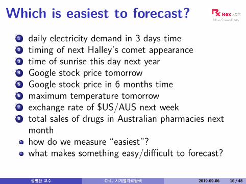
Which is easiest to forecast?1 daily electricity demand in 3 days time2 timing of next Halley’s comet appearance3 time of sunrise this day next year4 Google stock price tomorrow5 Google stock price in 6 months time6 maximum temperature tomorrow7 exchange rate of $US/AUS next week8 total sales of drugs in Australian pharmacies next
monthhow do we measure “easiest”?what makes something easy/difficult to forecast?
성병찬 교수 Ch1. 시계열자료탐색 2019-09-06 10 / 48

Factors affecting forecastability
Something is easier to forecast if:we have a good understanding of the factors thatcontribute to itthere is lots of data available;the forecasts cannot affect the thing we are trying toforecast.there is relatively low natural/unexplainable randomvariation.the future is somewhat similar to the past
성병찬 교수 Ch1. 시계열자료탐색 2019-09-06 11 / 48
Outline1 What can we forecast?
2 Time series data
3 The statistical forecasting perspective
4 Time plots
5 Seasonal plots
6 Lag plots and autocorrelation
7 White noise
성병찬 교수 Ch1. 시계열자료탐색 2019-09-06 12 / 48
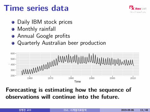
Time series dataDaily IBM stock pricesMonthly rainfallAnnual Google profitsQuarterly Australian beer production
200
300
400
500
600
1960 1970 1980 1990 2000 2010
Time
.
Forecasting is estimating how the sequence ofobservations will continue into the future.
성병찬 교수 Ch1. 시계열자료탐색 2019-09-06 13 / 48
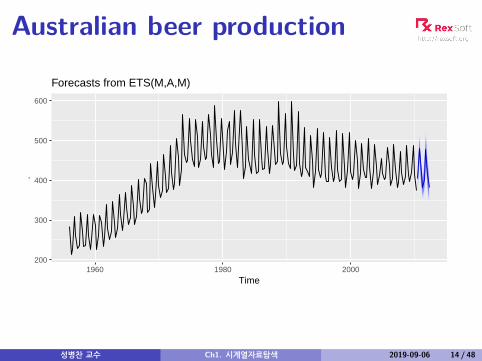
Australian beer production
200
300
400
500
600
1960 1980 2000
Time
.
Forecasts from ETS(M,A,M)
성병찬 교수 Ch1. 시계열자료탐색 2019-09-06 14 / 48

Australian beer production
350
400
450
500
1995 2000 2005 2010
Time
.
Forecasts from ETS(M,A,M)
성병찬 교수 Ch1. 시계열자료탐색 2019-09-06 15 / 48
Outline1 What can we forecast?
2 Time series data
3 The statistical forecasting perspective
4 Time plots
5 Seasonal plots
6 Lag plots and autocorrelation
7 White noise
성병찬 교수 Ch1. 시계열자료탐색 2019-09-06 16 / 48
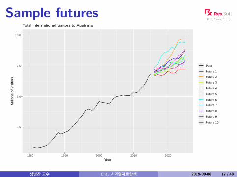
Sample futures
2.5
5.0
7.5
10.0
1980 1990 2000 2010 2020
Year
Mill
ions
of v
isito
rs
Data
Future 1
Future 2
Future 3
Future 4
Future 5
Future 6
Future 7
Future 8
Future 9
Future 10
Total international visitors to Australia
성병찬 교수 Ch1. 시계열자료탐색 2019-09-06 17 / 48
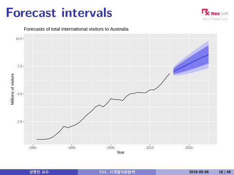
Forecast intervals
2.5
5.0
7.5
10.0
1980 1990 2000 2010 2020
Year
Mill
ions
of v
isito
rs
Forecasts of total international visitors to Australia
성병찬 교수 Ch1. 시계열자료탐색 2019-09-06 18 / 48
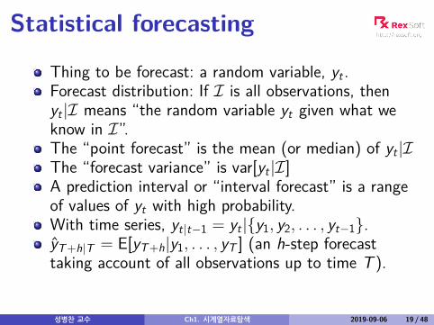
Statistical forecasting
Thing to be forecast: a random variable, yt .Forecast distribution: If I is all observations, thenyt |I means “the random variable yt given what weknow in I”.The “point forecast” is the mean (or median) of yt |IThe “forecast variance” is var[yt |I]A prediction interval or “interval forecast” is a rangeof values of yt with high probability.With time series, yt|t−1 = yt |{y1, y2, . . . , yt−1}.yT+h|T = E[yT+h|y1, . . . , yT ] (an h-step forecasttaking account of all observations up to time T ).
성병찬 교수 Ch1. 시계열자료탐색 2019-09-06 19 / 48
Outline1 What can we forecast?
2 Time series data
3 The statistical forecasting perspective
4 Time plots
5 Seasonal plots
6 Lag plots and autocorrelation
7 White noise
성병찬 교수 Ch1. 시계열자료탐색 2019-09-06 20 / 48
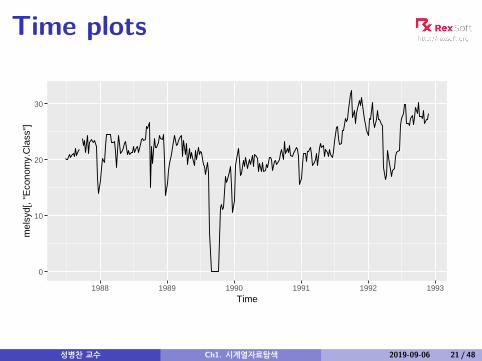
Time plots
0
10
20
30
1988 1989 1990 1991 1992 1993
Time
mel
syd[
, "E
cono
my.
Cla
ss"]
성병찬 교수 Ch1. 시계열자료탐색 2019-09-06 21 / 48
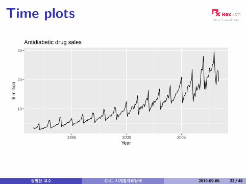
Time plots
10
20
30
1995 2000 2005
Year
$ m
illio
n
Antidiabetic drug sales
성병찬 교수 Ch1. 시계열자료탐색 2019-09-06 22 / 48
Outline1 What can we forecast?
2 Time series data
3 The statistical forecasting perspective
4 Time plots
5 Seasonal plots
6 Lag plots and autocorrelation
7 White noise
성병찬 교수 Ch1. 시계열자료탐색 2019-09-06 23 / 48
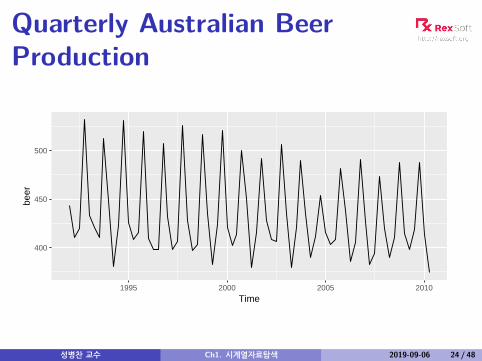
Quarterly Australian BeerProduction
400
450
500
1995 2000 2005 2010
Time
beer
성병찬 교수 Ch1. 시계열자료탐색 2019-09-06 24 / 48
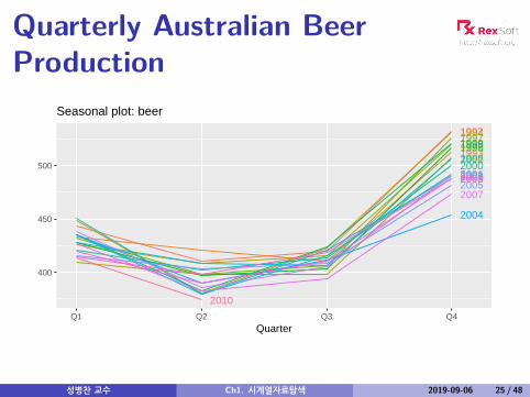
Quarterly Australian BeerProduction
1992
1993
199419951996
199719981999
200020012002
2003
2004
20052006
2007
20082009
2010
400
450
500
Q1 Q2 Q3 Q4
Quarter
Seasonal plot: beer
성병찬 교수 Ch1. 시계열자료탐색 2019-09-06 25 / 48
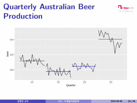
Quarterly Australian BeerProduction
400
450
500
Q1 Q2 Q3 Q4
Quarter
beer
성병찬 교수 Ch1. 시계열자료탐색 2019-09-06 26 / 48
Outline1 What can we forecast?
2 Time series data
3 The statistical forecasting perspective
4 Time plots
5 Seasonal plots
6 Lag plots and autocorrelation
7 White noise
성병찬 교수 Ch1. 시계열자료탐색 2019-09-06 27 / 48
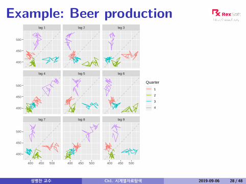
Example: Beer production
lag 7 lag 8 lag 9
lag 4 lag 5 lag 6
lag 1 lag 2 lag 3
400 450 500 400 450 500 400 450 500
400
450
500
400
450
500
400
450
500
Quarter
1
2
3
4
성병찬 교수 Ch1. 시계열자료탐색 2019-09-06 28 / 48

Lagged scatterplots
Each graph shows yt plotted against yt−k fordifferent values of k .The autocorrelations are the correlations associatedwith these scatterplots.
성병찬 교수 Ch1. 시계열자료탐색 2019-09-06 29 / 48
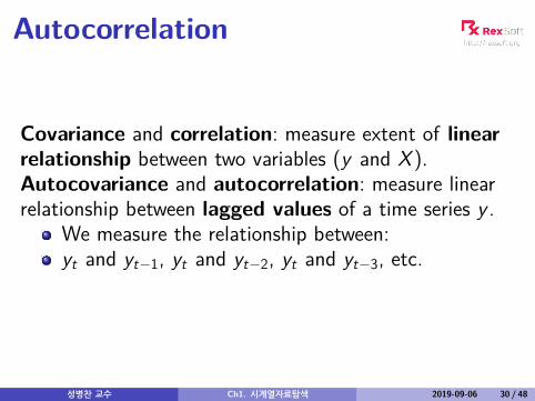
Autocorrelation
Covariance and correlation: measure extent of linearrelationship between two variables (y and X ).Autocovariance and autocorrelation: measure linearrelationship between lagged values of a time series y .
We measure the relationship between:yt and yt−1, yt and yt−2, yt and yt−3, etc.
성병찬 교수 Ch1. 시계열자료탐색 2019-09-06 30 / 48
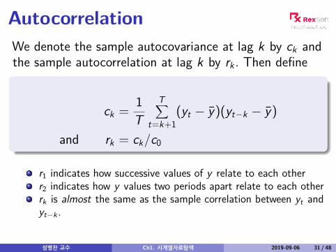
AutocorrelationWe denote the sample autocovariance at lag k by ck andthe sample autocorrelation at lag k by rk . Then define
ck = 1T
T∑t=k+1
(yt − y)(yt−k − y)
and rk = ck/c0
r1 indicates how successive values of y relate to each otherr2 indicates how y values two periods apart relate to each otherrk is almost the same as the sample correlation between yt andyt−k .
성병찬 교수 Ch1. 시계열자료탐색 2019-09-06 31 / 48
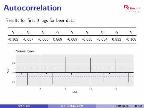
AutocorrelationResults for first 9 lags for beer data:
r1 r2 r3 r4 r5 r6 r7 r8 r9
-0.102 -0.657 -0.060 0.869 -0.089 -0.635 -0.054 0.832 -0.108
−0.5
0.0
0.5
4 8 12 16
Lag
AC
F
Series: beer
성병찬 교수 Ch1. 시계열자료탐색 2019-09-06 32 / 48
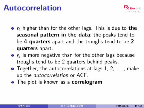
Autocorrelation
r4 higher than for the other lags. This is due to theseasonal pattern in the data: the peaks tend tobe 4 quarters apart and the troughs tend to be 2quarters apart.r2 is more negative than for the other lags becausetroughs tend to be 2 quarters behind peaks.Together, the autocorrelations at lags 1, 2, . . . , makeup the autocorrelation or ACF.The plot is known as a correlogram
성병찬 교수 Ch1. 시계열자료탐색 2019-09-06 33 / 48

ACF
−0.5
0.0
0.5
4 8 12 16
Lag
AC
F
Series: beer
성병찬 교수 Ch1. 시계열자료탐색 2019-09-06 34 / 48
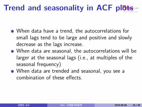
Trend and seasonality in ACF plots
When data have a trend, the autocorrelations forsmall lags tend to be large and positive and slowlydecrease as the lags increase.When data are seasonal, the autocorrelations will belarger at the seasonal lags (i.e., at multiples of theseasonal frequency)When data are trended and seasonal, you see acombination of these effects.
성병찬 교수 Ch1. 시계열자료탐색 2019-09-06 35 / 48
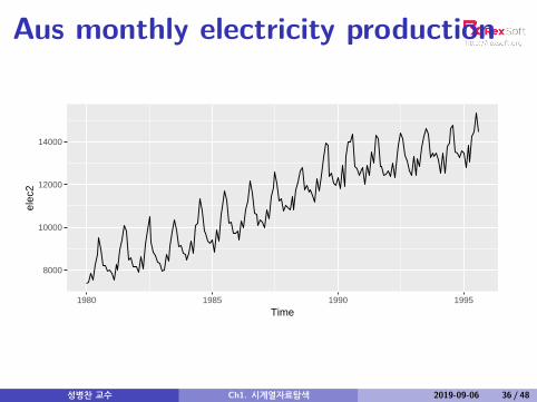
Aus monthly electricity production
8000
10000
12000
14000
1980 1985 1990 1995
Time
elec
2
성병찬 교수 Ch1. 시계열자료탐색 2019-09-06 36 / 48
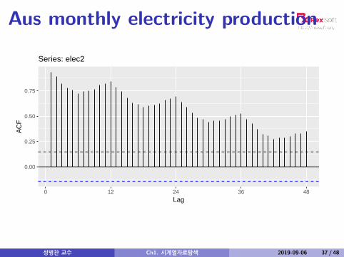
Aus monthly electricity production
0.00
0.25
0.50
0.75
0 12 24 36 48
Lag
AC
F
Series: elec2
성병찬 교수 Ch1. 시계열자료탐색 2019-09-06 37 / 48
Aus monthly electricity production
Time plot shows clear trend and seasonality.The same features are reflected in the ACF.
The slowly decaying ACF indicates trend.The ACF peaks at lags 12, 24, 36, . . . , indicateseasonality of length 12.
성병찬 교수 Ch1. 시계열자료탐색 2019-09-06 38 / 48
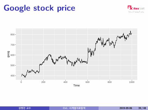
Google stock price
400
500
600
700
800
0 200 400 600 800 1000
Time
goog
성병찬 교수 Ch1. 시계열자료탐색 2019-09-06 39 / 48
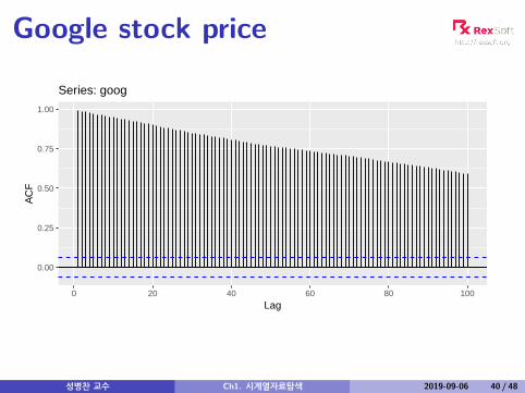
Google stock price
0.00
0.25
0.50
0.75
1.00
0 20 40 60 80 100
Lag
AC
F
Series: goog
성병찬 교수 Ch1. 시계열자료탐색 2019-09-06 40 / 48
Outline1 What can we forecast?
2 Time series data
3 The statistical forecasting perspective
4 Time plots
5 Seasonal plots
6 Lag plots and autocorrelation
7 White noise
성병찬 교수 Ch1. 시계열자료탐색 2019-09-06 41 / 48
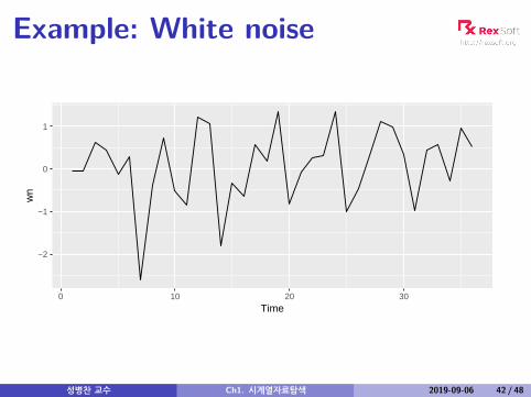
Example: White noise
−2
−1
0
1
0 10 20 30
Time
wn
성병찬 교수 Ch1. 시계열자료탐색 2019-09-06 42 / 48
Example: White noise
r1 -0.04r2 -0.26r3 -0.06r4 0.04r5 -0.01r6 0.13r7 0.12r8 -0.13r9 0.15
r10 -0.05
Sample autocorrelations for white noise series.We expect each autocorrelation to be close to zero.
성병찬 교수 Ch1. 시계열자료탐색 2019-09-06 43 / 48
−0.2
0.0
0.2
1 2 3 4 5 6 7 8 9 10 11 12 13 14 15Lag
AC
F
Series: wn

Sampling distribution of autocorrelations
Sampling distribution of rk for white noise data isasymptotically N(0,1/T ).
95% of all rk for white noise must lie within±1.96/
√T .
If this is not the case, the series is probably not WN.Common to plot lines at ±1.96/
√T when plotting
ACF. These are the {critical values}.
성병찬 교수 Ch1. 시계열자료탐색 2019-09-06 44 / 48
Autocorrelation
성병찬 교수 Ch1. 시계열자료탐색 2019-09-06 45 / 48
−0.2
0.0
0.2
1 2 3 4 5 6 7 8 9 10 11 12 13 14 15Lag
AC
F
Series: wnExample:T = 36 and so criticalvalues at±1.96/
√36 = ±0.327.
All autocorrelationcoefficients lie withinthese limits, confirmingthat the data are whitenoise. (More precisely,the data cannot bedistinguished from white noise.)
Example: Pigs slaughtered
80000
90000
100000
110000
1990 1991 1992 1993 1994 1995
Year
thou
sand
s
Number of pigs slaughtered in Victoria
성병찬 교수 Ch1. 시계열자료탐색 2019-09-06 46 / 48

Example: Pigs slaughtered
−0.2
0.0
0.2
12 246 18
Lag
AC
F
Series: pigs2
성병찬 교수 Ch1. 시계열자료탐색 2019-09-06 47 / 48
Example: Pigs slaughtered
Monthly total number of pigs slaughtered in the state ofVictoria, Australia, from January 1990 through August1995. (Source: Australian Bureau of Statistics.)
Difficult to detect pattern in time plot.ACF shows some significant autocorrelation at lags 1,2, and 3.r12 relatively large although not significant. This mayindicate some slight seasonality.
These show the series is not a white noise series.
성병찬 교수 Ch1. 시계열자료탐색 2019-09-06 48 / 48

Ch1-부록. 시계열자료탐색
성병찬 교수
중앙대 응용통계학과
2019-09-06
성병찬 교수 Ch1-부록. 시계열자료탐색 2019-09-06 1 / 26
Outline
1 Box-Cox transformations
2 Residual diagnostics
3 Evaluating forecast accuracy
성병찬 교수 Ch1-부록. 시계열자료탐색 2019-09-06 2 / 26
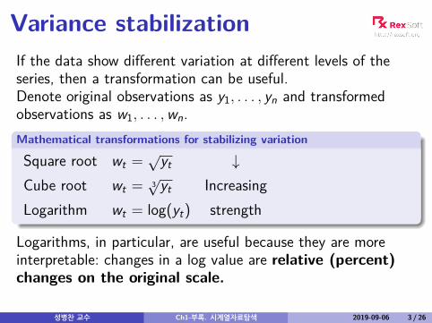
Variance stabilizationIf the data show different variation at different levels of theseries, then a transformation can be useful.Denote original observations as y1, . . . , yn and transformedobservations as w1, . . . ,wn.Mathematical transformations for stabilizing variation
Square root wt = √yt ↓Cube root wt = 3
√yt IncreasingLogarithm wt = log(yt) strength
Logarithms, in particular, are useful because they are moreinterpretable: changes in a log value are relative (percent)changes on the original scale.
성병찬 교수 Ch1-부록. 시계열자료탐색 2019-09-06 3 / 26
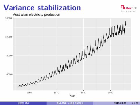
Variance stabilization
4000
8000
12000
16000
1960 1970 1980 1990Year
Australian electricity production
성병찬 교수 Ch1-부록. 시계열자료탐색 2019-09-06 4 / 26
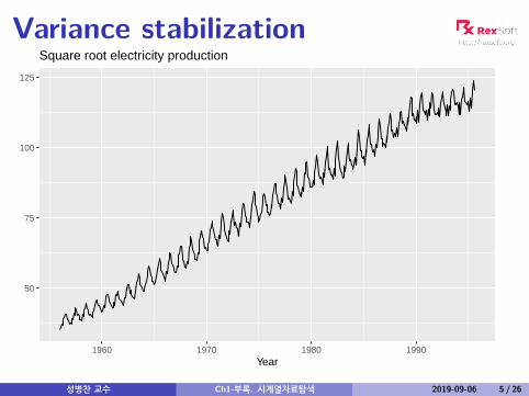
Variance stabilization
50
75
100
125
1960 1970 1980 1990Year
Square root electricity production
성병찬 교수 Ch1-부록. 시계열자료탐색 2019-09-06 5 / 26
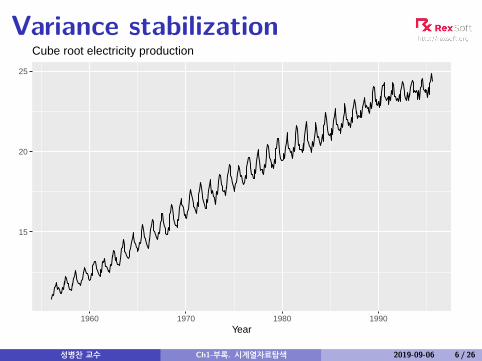
Variance stabilization
15
20
25
1960 1970 1980 1990Year
Cube root electricity production
성병찬 교수 Ch1-부록. 시계열자료탐색 2019-09-06 6 / 26

Variance stabilization
8
9
1960 1970 1980 1990Year
Log electricity production
성병찬 교수 Ch1-부록. 시계열자료탐색 2019-09-06 7 / 26
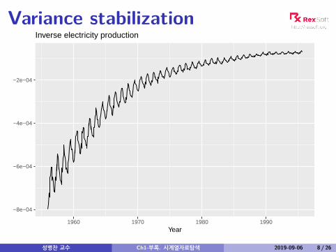
Variance stabilization
−8e−04
−6e−04
−4e−04
−2e−04
1960 1970 1980 1990Year
Inverse electricity production
성병찬 교수 Ch1-부록. 시계열자료탐색 2019-09-06 8 / 26
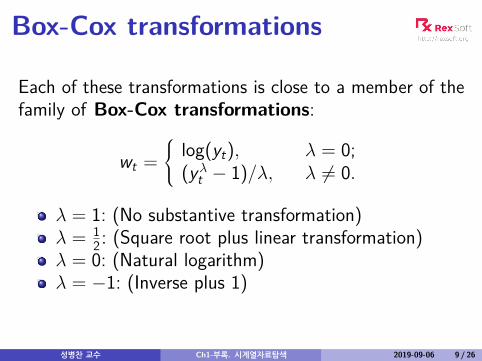
Box-Cox transformations
Each of these transformations is close to a member of thefamily of Box-Cox transformations:
wt = log(yt), λ = 0;
(yλt − 1)/λ, λ 6= 0.
λ = 1: (No substantive transformation)λ = 1
2 : (Square root plus linear transformation)λ = 0: (Natural logarithm)λ = −1: (Inverse plus 1)
성병찬 교수 Ch1-부록. 시계열자료탐색 2019-09-06 9 / 26
Outline
1 Box-Cox transformations
2 Residual diagnostics
3 Evaluating forecast accuracy
성병찬 교수 Ch1-부록. 시계열자료탐색 2019-09-06 10 / 26
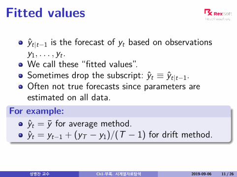
Fitted values
yt|t−1 is the forecast of yt based on observationsy1, . . . , yt .We call these “fitted values”.Sometimes drop the subscript: yt ≡ yt|t−1.Often not true forecasts since parameters areestimated on all data.
For example:yt = y for average method.yt = yt−1 + (yT − y1)/(T − 1) for drift method.
성병찬 교수 Ch1-부록. 시계열자료탐색 2019-09-06 11 / 26

Forecasting residuals
Residuals in forecasting: difference between observedvalue and its fitted value: et = yt − yt|t−1.
Assumptions1 {et} uncorrelated. If they aren’t, then information left in
residuals that should be used in computing forecasts.2 {et} have mean zero. If they don’t, then forecasts are
biased.Useful properties (for prediction intervals)
3 {et} have constant variance.4 {et} are normally distributed.
성병찬 교수 Ch1-부록. 시계열자료탐색 2019-09-06 12 / 26
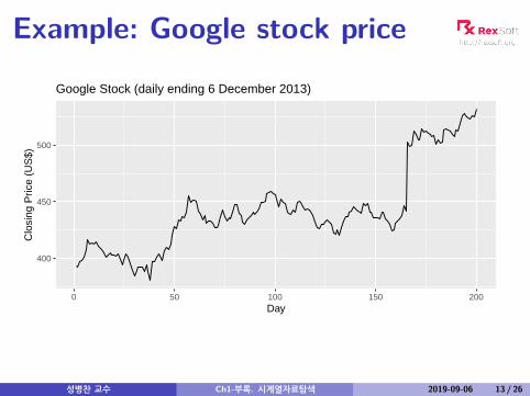
Example: Google stock price
400
450
500
0 50 100 150 200Day
Clo
sing
Pric
e (U
S$)
Google Stock (daily ending 6 December 2013)
성병찬 교수 Ch1-부록. 시계열자료탐색 2019-09-06 13 / 26
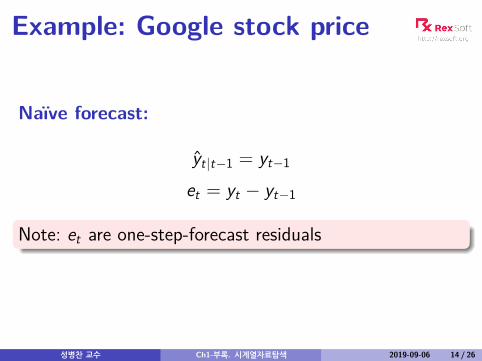
Example: Google stock price
Naïve forecast:
yt|t−1 = yt−1
et = yt − yt−1
Note: et are one-step-forecast residuals
성병찬 교수 Ch1-부록. 시계열자료탐색 2019-09-06 14 / 26
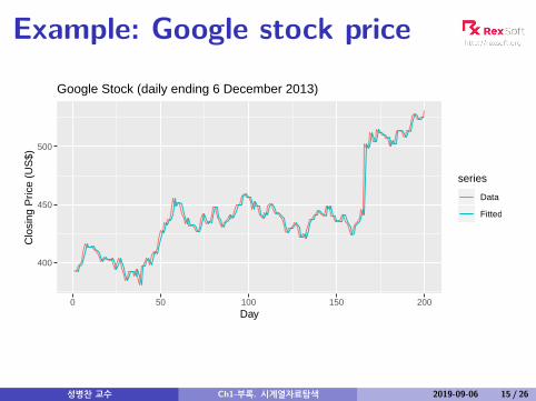
Example: Google stock price
400
450
500
0 50 100 150 200Day
Clo
sing
Pric
e (U
S$)
series
Data
Fitted
Google Stock (daily ending 6 December 2013)
성병찬 교수 Ch1-부록. 시계열자료탐색 2019-09-06 15 / 26
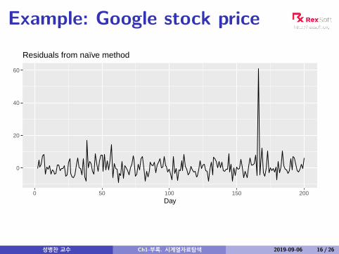
Example: Google stock price
0
20
40
60
0 50 100 150 200Day
Residuals from naïve method
성병찬 교수 Ch1-부록. 시계열자료탐색 2019-09-06 16 / 26
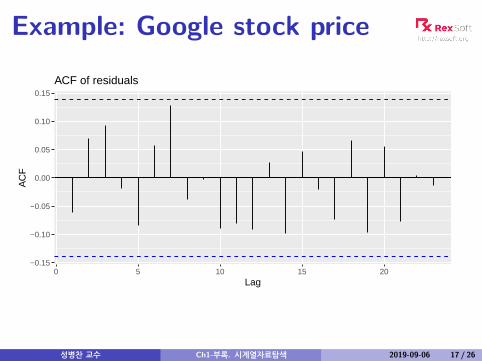
Example: Google stock price
−0.15
−0.10
−0.05
0.00
0.05
0.10
0.15
0 5 10 15 20Lag
AC
F
ACF of residuals
성병찬 교수 Ch1-부록. 시계열자료탐색 2019-09-06 17 / 26
ACF of residuals
We assume that the residuals are white noise(uncorrelated, mean zero, constant variance). If theyaren’t, then there is information left in the residualsthat should be used in computing forecasts.So a standard residual diagnostic is to check the ACFof the residuals of a forecasting method.We expect these to look like white noise.
성병찬 교수 Ch1-부록. 시계열자료탐색 2019-09-06 18 / 26
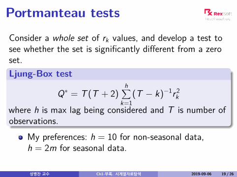
Portmanteau tests
Consider a whole set of rk values, and develop a test tosee whether the set is significantly different from a zeroset.Ljung-Box test
Q∗ = T (T + 2)h∑
k=1(T − k)−1r 2
k
where h is max lag being considered and T is number ofobservations.
My preferences: h = 10 for non-seasonal data,h = 2m for seasonal data.
성병찬 교수 Ch1-부록. 시계열자료탐색 2019-09-06 19 / 26
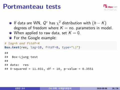
Portmanteau tests
If data are WN, Q∗ has χ2 distribution with (h − K )degrees of freedom where K = no. parameters in model.When applied to raw data, set K = 0.For the Google example:
# lag=h and fitdf=KBox.test(res, lag=10, fitdf=0, type="Lj")
#### Box-Ljung test#### data: res## X-squared = 11.031, df = 10, p-value = 0.3551
성병찬 교수 Ch1-부록. 시계열자료탐색 2019-09-06 20 / 26
Outline
1 Box-Cox transformations
2 Residual diagnostics
3 Evaluating forecast accuracy
성병찬 교수 Ch1-부록. 시계열자료탐색 2019-09-06 21 / 26
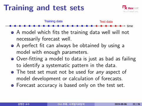
Training and test sets
time
Training data Test data
A model which fits the training data well will notnecessarily forecast well.A perfect fit can always be obtained by using amodel with enough parameters.Over-fitting a model to data is just as bad as failingto identify a systematic pattern in the data.The test set must not be used for any aspect ofmodel development or calculation of forecasts.Forecast accuracy is based only on the test set.
성병찬 교수 Ch1-부록. 시계열자료탐색 2019-09-06 22 / 26

Forecast errors
Forecast “error”: the difference between an observed valueand its forecast.
eT+h = yT+h − yT+h|T ,
where the training data is given by {y1, . . . , yT}Unlike residuals, forecast errors on the test setinvolve multi-step forecasts.These are true forecast errors as the test data is notused in computing yT+h|T .
성병찬 교수 Ch1-부록. 시계열자료탐색 2019-09-06 23 / 26
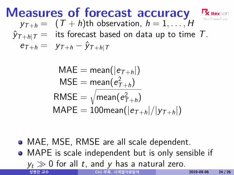
Measures of forecast accuracyyT+h = (T + h)th observation, h = 1, . . . ,H
yT+h|T = its forecast based on data up to time T .eT+h = yT+h − yT+h|T
MAE = mean(|eT+h|)MSE = mean(e2
T+h)RMSE =
√mean(e2
T+h)MAPE = 100mean(|eT+h|/|yT+h|)
MAE, MSE, RMSE are all scale dependent.MAPE is scale independent but is only sensible ifyt � 0 for all t, and y has a natural zero.성병찬 교수 Ch1-부록. 시계열자료탐색 2019-09-06 24 / 26
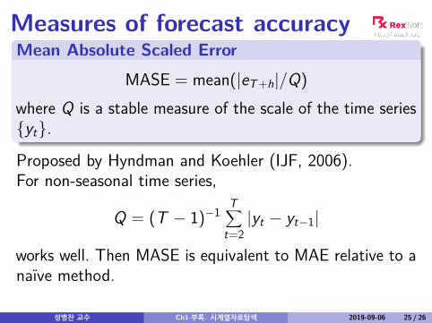
Measures of forecast accuracyMean Absolute Scaled Error
MASE = mean(|eT+h|/Q)where Q is a stable measure of the scale of the time series{yt}.
Proposed by Hyndman and Koehler (IJF, 2006).For non-seasonal time series,
Q = (T − 1)−1T∑
t=2|yt − yt−1|
works well. Then MASE is equivalent to MAE relative to anaïve method.
성병찬 교수 Ch1-부록. 시계열자료탐색 2019-09-06 25 / 26
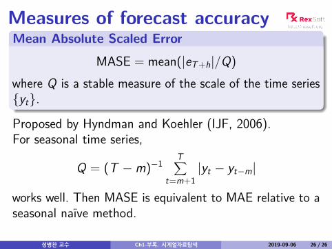
Measures of forecast accuracyMean Absolute Scaled Error
MASE = mean(|eT+h|/Q)where Q is a stable measure of the scale of the time series{yt}.
Proposed by Hyndman and Koehler (IJF, 2006).For seasonal time series,
Q = (T −m)−1T∑
t=m+1|yt − yt−m|
works well. Then MASE is equivalent to MAE relative to aseasonal naïve method.
성병찬 교수 Ch1-부록. 시계열자료탐색 2019-09-06 26 / 26
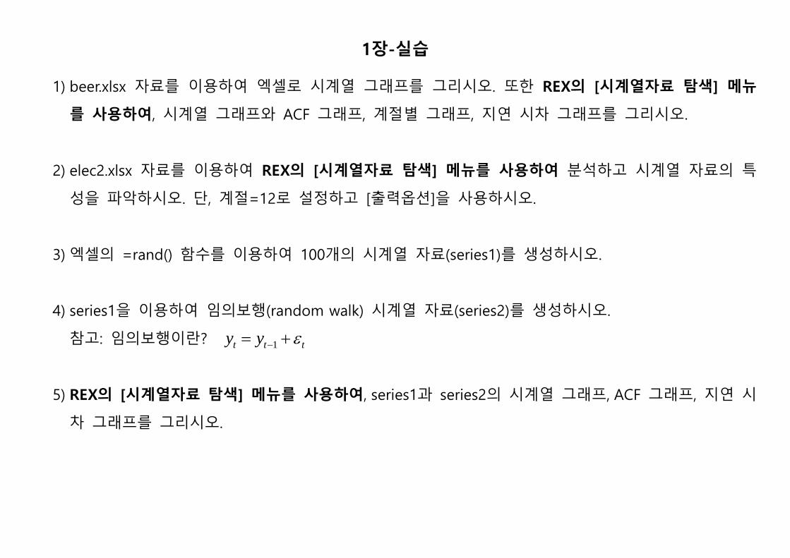
1장-실습
1) beer.xlsx 자료를 이용하여 엑셀로 시계열 그래프를 그리시오. 또한 REX의 [시계열자료 탐색] 메뉴
를 사용하여, 시계열 그래프와 ACF 그래프, 계절별 그래프, 지연 시차 그래프를 그리시오.
2) elec2.xlsx 자료를 이용하여 REX의 [시계열자료 탐색] 메뉴를 사용하여 분석하고 시계열 자료의 특
성을 파악하시오. 단, 계절=12로 설정하고 [출력옵션]을 사용하시오.
3) 엑셀의 =rand() 함수를 이용하여 100개의 시계열 자료(series1)를 생성하시오.
4) series1을 이용하여 임의보행(random walk) 시계열 자료(series2)를 생성하시오.
참고: 임의보행이란? 1t t ty y −= +
5) REX의 [시계열자료 탐색] 메뉴를 사용하여, series1과 series2의 시계열 그래프, ACF 그래프, 지연 시
차 그래프를 그리시오.

Ch2. ARIMA 분석
성병찬 교수
중앙대 응용통계학과
2019-09-06
성병찬 교수 Ch2. ARIMA 분석 2019-09-06 1 / 54

Outline
1 Stationarity and differencing
2 Non-seasonal ARIMA models
3 Order selection
성병찬 교수 Ch2. ARIMA 분석 2019-09-06 2 / 54
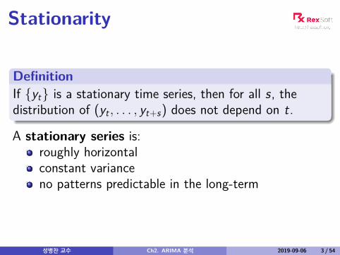
Stationarity
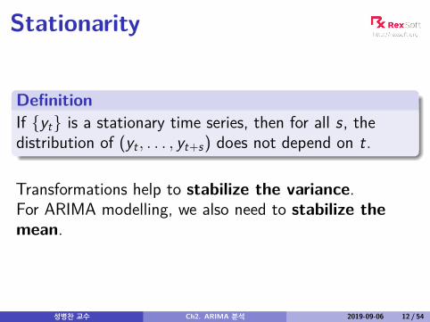
DefinitionIf {yt} is a stationary time series, then for all s, thedistribution of (yt , . . . , yt+s) does not depend on t.
A stationary series is:roughly horizontalconstant varianceno patterns predictable in the long-term
성병찬 교수 Ch2. ARIMA 분석 2019-09-06 3 / 54
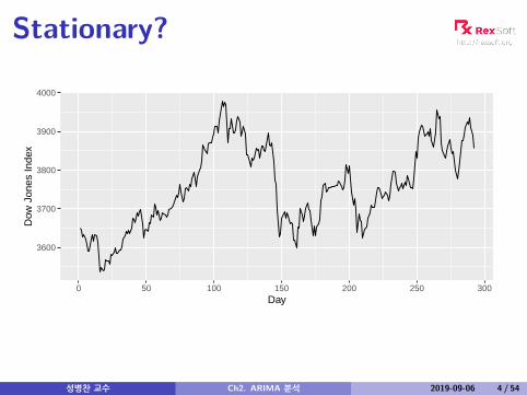
Stationary?
3600
3700
3800
3900
4000
0 50 100 150 200 250 300Day
Dow
Jon
es In
dex
성병찬 교수 Ch2. ARIMA 분석 2019-09-06 4 / 54
Stationary?
−100
−50
0
50
0 50 100 150 200 250 300Day
Cha
nge
in D
ow J
ones
Inde
x
성병찬 교수 Ch2. ARIMA 분석 2019-09-06 5 / 54

Stationary?
4000
5000
6000
1950 1955 1960 1965 1970 1975 1980Year
Num
ber
of s
trik
es
성병찬 교수 Ch2. ARIMA 분석 2019-09-06 6 / 54
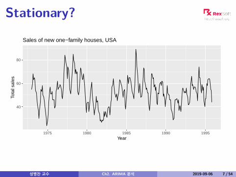
Stationary?
40
60
80
1975 1980 1985 1990 1995Year
Tota
l sal
es
Sales of new one−family houses, USA
성병찬 교수 Ch2. ARIMA 분석 2019-09-06 7 / 54
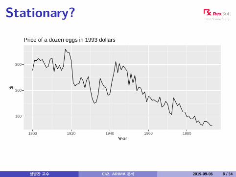
Stationary?
100
200
300
1900 1920 1940 1960 1980Year
$
Price of a dozen eggs in 1993 dollars
성병찬 교수 Ch2. ARIMA 분석 2019-09-06 8 / 54
Stationary?
80
90
100
110
1990 1991 1992 1993 1994 1995Year
thou
sand
s
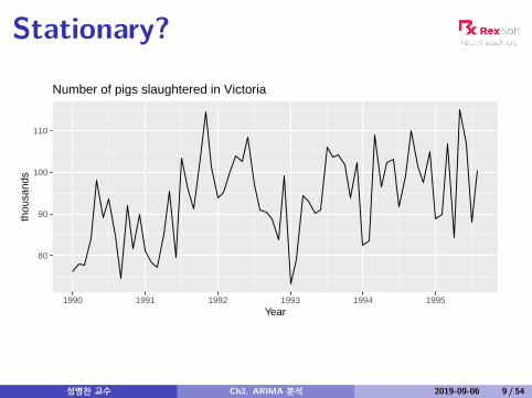
Number of pigs slaughtered in Victoria
성병찬 교수 Ch2. ARIMA 분석 2019-09-06 9 / 54
Stationary?
0
2000
4000
6000
1820 1840 1860 1880 1900 1920Year
Num
ber
trap
ped
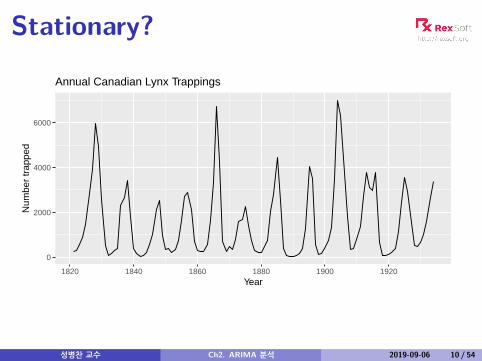
Annual Canadian Lynx Trappings
성병찬 교수 Ch2. ARIMA 분석 2019-09-06 10 / 54
Stationary?
400
450
500
1995 2000 2005 2010Year
meg
alitr
es
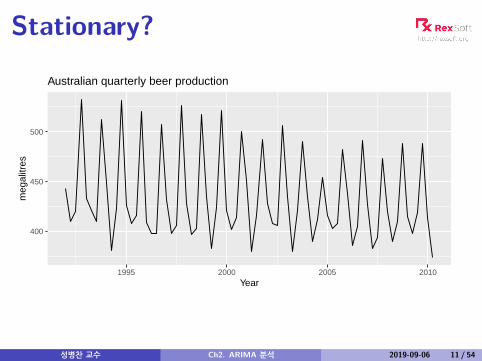
Australian quarterly beer production
성병찬 교수 Ch2. ARIMA 분석 2019-09-06 11 / 54
Stationarity
DefinitionIf {yt} is a stationary time series, then for all s, thedistribution of (yt , . . . , yt+s) does not depend on t.
Transformations help to stabilize the variance.For ARIMA modelling, we also need to stabilize themean.
성병찬 교수 Ch2. ARIMA 분석 2019-09-06 12 / 54

Non-stationarity in the mean
Identifying non-stationary seriestime plot.The ACF of stationary data drops to zero relativelyquicklyThe ACF of non-stationary data decreases slowly.For non-stationary data, the value of r1 is often largeand positive.
성병찬 교수 Ch2. ARIMA 분석 2019-09-06 13 / 54
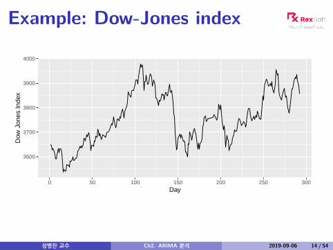
Example: Dow-Jones index
3600
3700
3800
3900
4000
0 50 100 150 200 250 300Day
Dow
Jon
es In
dex
성병찬 교수 Ch2. ARIMA 분석 2019-09-06 14 / 54
Example: Dow-Jones index
0.00
0.25
0.50
0.75
1.00
0 5 10 15 20 25Lag
AC
F
Series: dj
성병찬 교수 Ch2. ARIMA 분석 2019-09-06 15 / 54

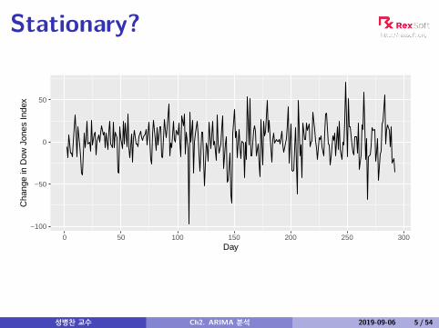
Example: Dow-Jones index
−100
−50
0
50
0 50 100 150 200 250 300Day
Cha
nge
in D
ow J
ones
Inde
x
성병찬 교수 Ch2. ARIMA 분석 2019-09-06 16 / 54

Example: Dow-Jones index
−0.10
−0.05
0.00
0.05
0.10
0 5 10 15 20 25Lag
AC
F
Series: diff(dj)
성병찬 교수 Ch2. ARIMA 분석 2019-09-06 17 / 54
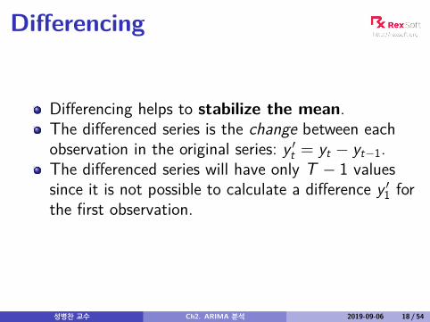
Differencing
Differencing helps to stabilize the mean.The differenced series is the change between eachobservation in the original series: y ′t = yt − yt−1.The differenced series will have only T − 1 valuessince it is not possible to calculate a difference y ′1 forthe first observation.
성병찬 교수 Ch2. ARIMA 분석 2019-09-06 18 / 54

Second-order differencing
Occasionally the differenced data will not appearstationary and it may be necessary to difference the dataa second time:
y ′′t = y ′t − y ′t−1= (yt − yt−1)− (yt−1 − yt−2)= yt − 2yt−1 + yt−2.
y ′′t will have T − 2 values.In practice, it is almost never necessary to go beyondsecond-order differences.
성병찬 교수 Ch2. ARIMA 분석 2019-09-06 19 / 54
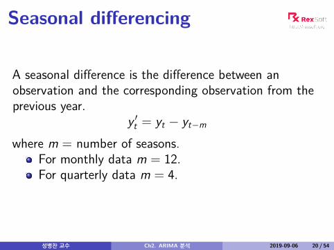
Seasonal differencing
A seasonal difference is the difference between anobservation and the corresponding observation from theprevious year.
y ′t = yt − yt−m
where m = number of seasons.For monthly data m = 12.For quarterly data m = 4.
성병찬 교수 Ch2. ARIMA 분석 2019-09-06 20 / 54
Electricity production
200
300
400
1980 1990 2000 2010Time
.
성병찬 교수 Ch2. ARIMA 분석 2019-09-06 21 / 54

Electricity production
5.1
5.4
5.7
6.0
1980 1990 2000 2010Time
.
성병찬 교수 Ch2. ARIMA 분석 2019-09-06 22 / 54

Electricity production
0.0
0.1
1980 1990 2000 2010Time
.
성병찬 교수 Ch2. ARIMA 분석 2019-09-06 23 / 54
Electricity production
−0.15
−0.10
−0.05
0.00
0.05
0.10
1980 1990 2000 2010Time
.
성병찬 교수 Ch2. ARIMA 분석 2019-09-06 24 / 54

Electricity productionSeasonally differenced series is closer to beingstationary.Remaining non-stationarity can be removed withfurther first difference.
If y ′t = yt − yt−12 denotes seasonally differenced series,then twice-differenced series is
y ∗t = y ′t − y ′t−1= (yt − yt−12)− (yt−1 − yt−13)= yt − yt−1 − yt−12 + yt−13 .
성병찬 교수 Ch2. ARIMA 분석 2019-09-06 25 / 54
Seasonal differencing
When both seasonal and first differences are applied. . .it makes no difference which is done first—the resultwill be the same.If seasonality is strong, we recommend that seasonaldifferencing be done first because sometimes theresulting series will be stationary and there will be noneed for further first difference.
It is important that if differencing is used, the differencesare interpretable.
성병찬 교수 Ch2. ARIMA 분석 2019-09-06 26 / 54
Interpretation of differencing
first differences are the change between oneobservation and the next;seasonal differences are the change between oneyear to the next.
But taking lag 3 differences for yearly data, for example,results in a model which cannot be sensibly interpreted.
성병찬 교수 Ch2. ARIMA 분석 2019-09-06 27 / 54
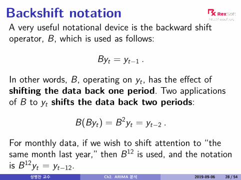
Backshift notationA very useful notational device is the backward shiftoperator, B, which is used as follows:
Byt = yt−1 .
In other words, B, operating on yt , has the effect ofshifting the data back one period. Two applicationsof B to yt shifts the data back two periods:
B(Byt) = B2yt = yt−2 .
For monthly data, if we wish to shift attention to “thesame month last year,” then B12 is used, and the notationis B12yt = yt−12.
성병찬 교수 Ch2. ARIMA 분석 2019-09-06 28 / 54
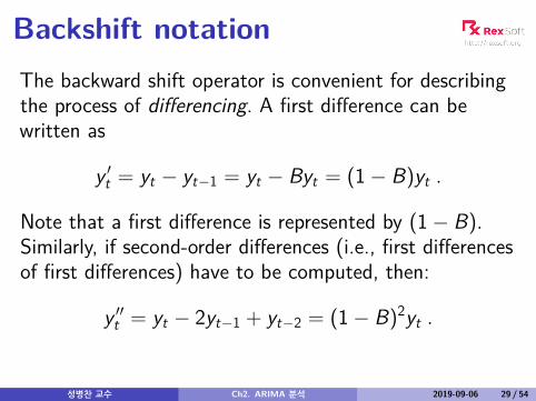
Backshift notationThe backward shift operator is convenient for describingthe process of differencing. A first difference can bewritten as
y ′t = yt − yt−1 = yt − Byt = (1− B)yt .
Note that a first difference is represented by (1− B).Similarly, if second-order differences (i.e., first differencesof first differences) have to be computed, then:
y ′′t = yt − 2yt−1 + yt−2 = (1− B)2yt .
성병찬 교수 Ch2. ARIMA 분석 2019-09-06 29 / 54

Backshift notationSecond-order difference is denoted (1− B)2.Second-order difference is not the same as a seconddifference, which would be denoted 1− B2;In general, a dth-order difference can be written as
(1− B)dyt .
A seasonal difference followed by a first differencecan be written as
(1− B)(1− Bm)yt .
성병찬 교수 Ch2. ARIMA 분석 2019-09-06 30 / 54
Backshift notation
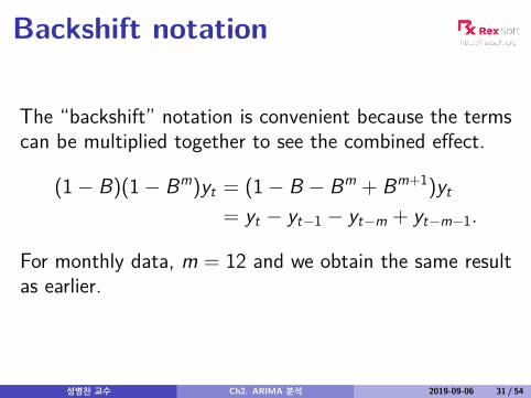
The “backshift” notation is convenient because the termscan be multiplied together to see the combined effect.
(1− B)(1− Bm)yt = (1− B − Bm + Bm+1)yt
= yt − yt−1 − yt−m + yt−m−1.
For monthly data, m = 12 and we obtain the same resultas earlier.
성병찬 교수 Ch2. ARIMA 분석 2019-09-06 31 / 54
Outline
1 Stationarity and differencing
2 Non-seasonal ARIMA models
3 Order selection
성병찬 교수 Ch2. ARIMA 분석 2019-09-06 32 / 54

Autoregressive modelsAutoregressive (AR) models:
yt = c + φ1yt−1 + φ2yt−2 + · · ·+ φpyt−p + εt ,
where εt is white noise. This is a multiple regression withlagged values of yt as predictors.
8
10
12
0 20 40 60 80 100Time
AR(1)
15.0
17.5
20.0
22.5
25.0
0 20 40 60 80 100Time
AR(2)
성병찬 교수 Ch2. ARIMA 분석 2019-09-06 33 / 54
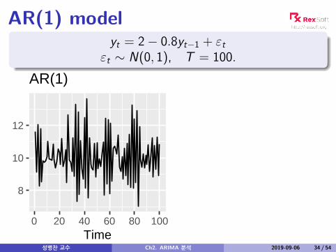
AR(1) modelyt = 2− 0.8yt−1 + εt
εt ∼ N(0, 1), T = 100.
8
10
12
0 20 40 60 80 100Time
AR(1)
성병찬 교수 Ch2. ARIMA 분석 2019-09-06 34 / 54
AR(1) model
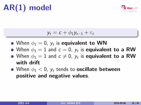
yt = c + φ1yt−1 + εt
When φ1 = 0, yt is equivalent to WNWhen φ1 = 1 and c = 0, yt is equivalent to a RWWhen φ1 = 1 and c 6= 0, yt is equivalent to a RWwith driftWhen φ1 < 0, yt tends to oscillate betweenpositive and negative values.
성병찬 교수 Ch2. ARIMA 분석 2019-09-06 35 / 54

AR(2) modelyt = 8 + 1.3yt−1 − 0.7yt−2 + εtεt ∼ N(0, 1), T = 100.
15.0
17.5
20.0
22.5
25.0
0 20 40 60 80 100Time
AR(2)
성병찬 교수 Ch2. ARIMA 분석 2019-09-06 36 / 54

Moving Average (MA) modelsMoving Average (MA) models:
yt = c + εt + θ1εt−1 + θ2εt−2 + · · ·+ θqεt−q,
where εt is white noise. This is a multiple regression with pasterrors as predictors. Don’t confuse this with moving averagesmoothing!
18
20
22
0 20 40 60 80 100Time
MA(1)
−5.0
−2.5
0.0
2.5
0 20 40 60 80 100Time
MA(2)
성병찬 교수 Ch2. ARIMA 분석 2019-09-06 37 / 54
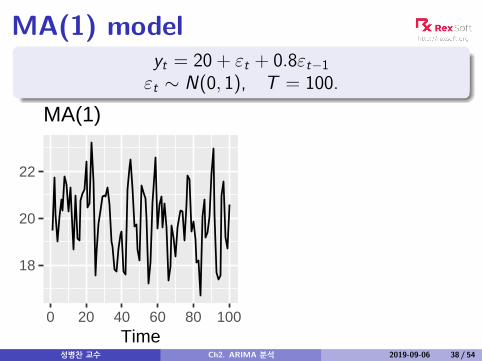
MA(1) modelyt = 20 + εt + 0.8εt−1εt ∼ N(0, 1), T = 100.
18
20
22
0 20 40 60 80 100Time
MA(1)
성병찬 교수 Ch2. ARIMA 분석 2019-09-06 38 / 54
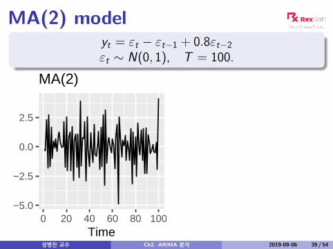
MA(2) modelyt = εt − εt−1 + 0.8εt−2εt ∼ N(0, 1), T = 100.
−5.0
−2.5
0.0
2.5
0 20 40 60 80 100Time
MA(2)
성병찬 교수 Ch2. ARIMA 분석 2019-09-06 39 / 54

MA(∞) modelsIt is possible to write any stationary AR(p) process as anMA(∞) process.Example: AR(1)yt = φ1yt−1 + εt
= φ1(φ1yt−2 + εt−1) + εt
= φ21yt−2 + φ1εt−1 + εt
= φ31yt−3 + φ2
1εt−2 + φ1εt−1 + εt
. . .
Provided −1 < φ1 < 1:
yt = εt + φ1εt−1 + φ21εt−2 + φ3
1εt−3 + · · ·
성병찬 교수 Ch2. ARIMA 분석 2019-09-06 40 / 54

ARIMA modelsAutoregressive Moving Average models:
yt = c + φ1yt−1 + · · ·+ φpyt−p
+ θ1εt−1 + · · ·+ θqεt−q + εt .
Predictors include both lagged values of yt andlagged errors.Conditions on coefficients ensure stationarity.Conditions on coefficients ensure invertibility.
Autoregressive Integrated Moving Average modelsCombine ARMA model with differencing.(1− B)dyt follows an ARMA model.성병찬 교수 Ch2. ARIMA 분석 2019-09-06 41 / 54
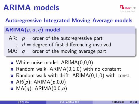
ARIMA modelsAutoregressive Integrated Moving Average modelsARIMA(p, d , q) modelAR: p = order of the autoregressive part
I: d = degree of first differencing involvedMA: q = order of the moving average part.
White noise model: ARIMA(0,0,0)Random walk: ARIMA(0,1,0) with no constantRandom walk with drift: ARIMA(0,1,0) with const.AR(p): ARIMA(p,0,0)MA(q): ARIMA(0,0,q)
성병찬 교수 Ch2. ARIMA 분석 2019-09-06 42 / 54

Backshift notation for ARIMAARMA model:
yt = c + φ1Byt + · · ·+ φpBpyt + εt + θ1Bεt + · · ·+ θqBqεt
or (1− φ1B − · · · − φpBp)yt = c + (1 + θ1B + · · ·+ θqBq)εt
ARIMA(1,1,1) model:
(1− φ1B) (1− B)yt = c + (1 + θ1B)εt↑ ↑ ↑
AR(1) First MA(1)difference
Written out:
yt = c + yt−1 + φ1yt−1 − φ1yt−2 + θ1εt−1 + εt
성병찬 교수 Ch2. ARIMA 분석 2019-09-06 43 / 54
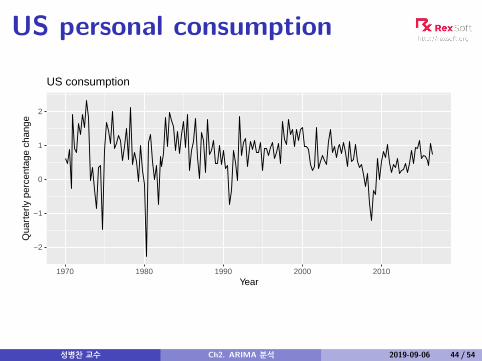
US personal consumption
−2
−1
0
1
2
1970 1980 1990 2000 2010Year
Qua
rter
ly p
erce
ntag
e ch
ange
US consumption
성병찬 교수 Ch2. ARIMA 분석 2019-09-06 44 / 54
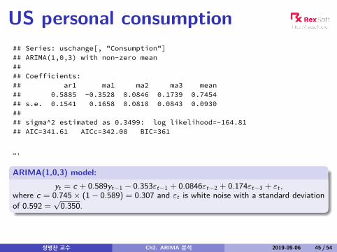
US personal consumption## Series: uschange[, "Consumption"]## ARIMA(1,0,3) with non-zero mean#### Coefficients:## ar1 ma1 ma2 ma3 mean## 0.5885 -0.3528 0.0846 0.1739 0.7454## s.e. 0.1541 0.1658 0.0818 0.0843 0.0930#### sigma^2 estimated as 0.3499: log likelihood=-164.81## AIC=341.61 AICc=342.08 BIC=361
“‘
ARIMA(1,0,3) model:yt = c + 0.589yt−1 − 0.353εt−1 + 0.0846εt−2 + 0.174εt−3 + εt ,
where c = 0.745× (1− 0.589) = 0.307 and εt is white noise with a standard deviationof 0.592 =
√0.350.
성병찬 교수 Ch2. ARIMA 분석 2019-09-06 45 / 54
US personal consumption
−1
0
1
2
2000 2005 2010 2015 2020Time
usch
ange
[, "C
onsu
mpt
ion"
]
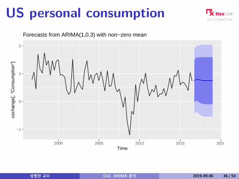
Forecasts from ARIMA(1,0,3) with non−zero mean
성병찬 교수 Ch2. ARIMA 분석 2019-09-06 46 / 54

Outline
1 Stationarity and differencing
2 Non-seasonal ARIMA models
3 Order selection
성병찬 교수 Ch2. ARIMA 분석 2019-09-06 47 / 54
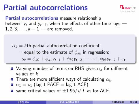
Partial autocorrelationsPartial autocorrelations measure relationshipbetween yt and yt−k , when the effects of other time lags —1, 2, 3, . . . , k − 1 — are removed.
αk = kth partial autocorrelation coefficient= equal to the estimate of φkk in regression:yt = φk0 + φk1yt−1 + φk2yt−2 + · · ·+ φkkyt−k + εt .
Varying number of terms on RHS gives αk for differentvalues of k .There are more efficient ways of calculating αk .α1 = ρ1 (lag-1 PACF = lag-1 ACF)same critical values of ±1.96/
√T as for ACF.
성병찬 교수 Ch2. ARIMA 분석 2019-09-06 48 / 54
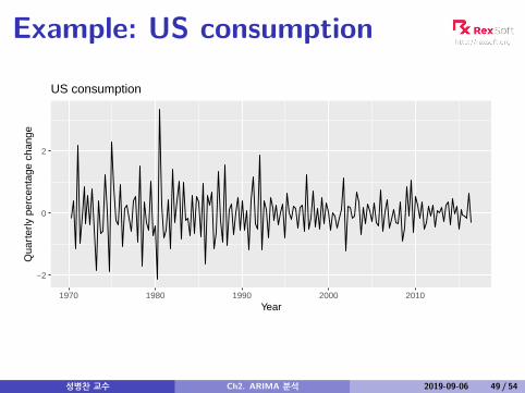
Example: US consumption
−2
0
2
1970 1980 1990 2000 2010Year
Qua
rter
ly p
erce
ntag
e ch
ange
US consumption
성병찬 교수 Ch2. ARIMA 분석 2019-09-06 49 / 54
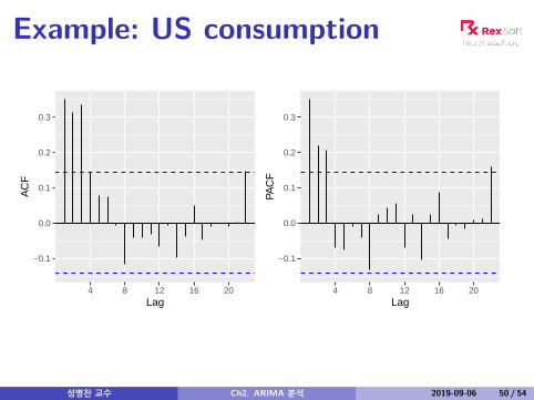
Example: US consumption
−0.1
0.0
0.1
0.2
0.3
4 8 12 16 20Lag
AC
F
−0.1
0.0
0.1
0.2
0.3
4 8 12 16 20Lag
PAC
F
성병찬 교수 Ch2. ARIMA 분석 2019-09-06 50 / 54
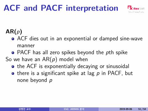
ACF and PACF interpretation
AR(p)ACF dies out in an exponential or damped sine-wavemannerPACF has all zero spikes beyond the pth spike
So we have an AR(p) model whenthe ACF is exponentially decaying or sinusoidalthere is a significant spike at lag p in PACF, butnone beyond p
성병찬 교수 Ch2. ARIMA 분석 2019-09-06 51 / 54
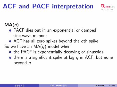
ACF and PACF interpretation
MA(q)PACF dies out in an exponential or dampedsine-wave mannerACF has all zero spikes beyond the qth spike
So we have an MA(q) model whenthe PACF is exponentially decaying or sinusoidalthere is a significant spike at lag q in ACF, but nonebeyond q
성병찬 교수 Ch2. ARIMA 분석 2019-09-06 52 / 54
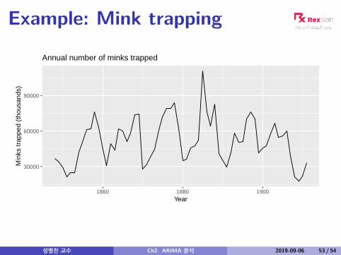
Example: Mink trapping
30000
60000
90000
1860 1880 1900Year
Min
ks tr
appe
d (t
hous
ands
)
Annual number of minks trapped
성병찬 교수 Ch2. ARIMA 분석 2019-09-06 53 / 54
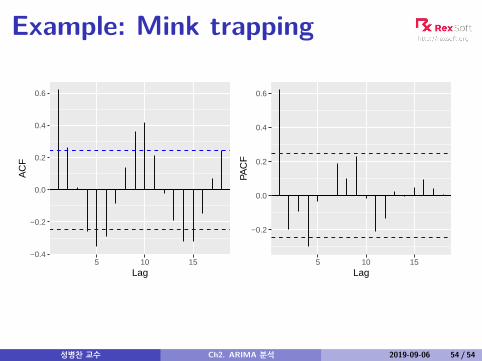
Example: Mink trapping
−0.4
−0.2
0.0
0.2
0.4
0.6
5 10 15Lag
AC
F
−0.2
0.0
0.2
0.4
0.6
5 10 15Lag
PAC
F
성병찬 교수 Ch2. ARIMA 분석 2019-09-06 54 / 54

2장-실습
1) dj.xlsx 파일의 시계열 자료를 [ARIMA 모형]으로 분석하시오.
([비계절 및 계절 차수 자동 선택] 옵션 및 [출력옵션] 탭을 이용)
A. 어떤 모형이 적합되었는가?
B. 잔차는 백색잡음의 가정을 만족하는가?
C. 예측치는 어떤 특징을 가지는가?
2) usmelec.xlsx 파일의 시계열 자료를 [ARIMA 모형]으로 분석하시오.
3) 엑셀 워크시트에 AR(1)과 MA(1)을 따르는 시계열을 각각 생성하시오.
4) ACF와 PACF의 특징을 관찰하고, 이론적 특성과 어떻게 다른지 설명하시오.

Ch3. 지수평활법 분석
성병찬 교수
중앙대 응용통계학과
2019-09-06
성병찬 교수 Ch3. 지수평활법 분석 2019-09-06 1 / 21
Outline
1 Simple exponential smoothing
2 Trend methods
3 Seasonal methods
성병찬 교수 Ch3. 지수평활법 분석 2019-09-06 2 / 21

Simple methodsTime series y1, y2, . . . , yT .Random walk forecasts
yT+h|T = yT
Average forecasts
yT+h|T = 1T
T∑t=1
yt
Want something in between that weights most recentdata more highly.Simple exponential smoothing uses a weighted movingaverage with weights that decrease exponentially.
성병찬 교수 Ch3. 지수평활법 분석 2019-09-06 3 / 21
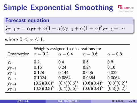
Simple Exponential SmoothingForecast equationyT+1|T = αyT + α(1− α)yT−1 + α(1− α)2yT−2 + · · ·
where 0 ≤ α ≤ 1.Weights assigned to observations for:
Observation α = 0.2 α = 0.4 α = 0.6 α = 0.8
yT 0.2 0.4 0.6 0.8yT−1 0.16 0.24 0.24 0.16yT−2 0.128 0.144 0.096 0.032yT−3 0.1024 0.0864 0.0384 0.0064yT−4 (0.2)(0.8)4 (0.4)(0.6)4 (0.6)(0.4)4 (0.8)(0.2)4
yT−5 (0.2)(0.8)5 (0.4)(0.6)5 (0.6)(0.4)5 (0.8)(0.2)5
성병찬 교수 Ch3. 지수평활법 분석 2019-09-06 4 / 21
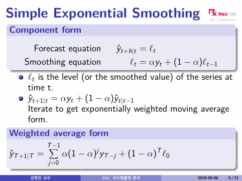
Simple Exponential SmoothingComponent form
Forecast equation yt+h|t = `t
Smoothing equation `t = αyt + (1− α)`t−1
`t is the level (or the smoothed value) of the series attime t.yt+1|t = αyt + (1− α)yt|t−1Iterate to get exponentially weighted moving averageform.
Weighted average form
yT+1|T =T−1∑j=0
α(1− α)jyT−j + (1− α)T `0
성병찬 교수 Ch3. 지수평활법 분석 2019-09-06 5 / 21
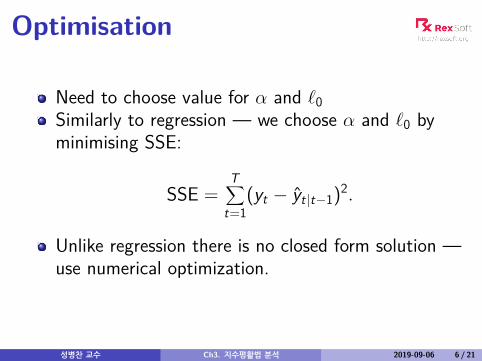
Optimisation
Need to choose value for α and `0Similarly to regression — we choose α and `0 byminimising SSE:
SSE =T∑
t=1(yt − yt|t−1)2.
Unlike regression there is no closed form solution —use numerical optimization.
성병찬 교수 Ch3. 지수평활법 분석 2019-09-06 6 / 21
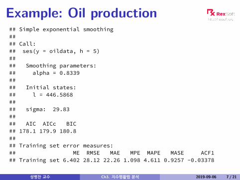
Example: Oil production## Simple exponential smoothing#### Call:## ses(y = oildata, h = 5)#### Smoothing parameters:## alpha = 0.8339#### Initial states:## l = 446.5868#### sigma: 29.83#### AIC AICc BIC## 178.1 179.9 180.8#### Training set error measures:## ME RMSE MAE MPE MAPE MASE ACF1## Training set 6.402 28.12 22.26 1.098 4.611 0.9257 -0.03378
성병찬 교수 Ch3. 지수평활법 분석 2019-09-06 7 / 21

Example: Oil productionYear Time Observation Level Forecast
t yt `t yt+1|t1995 0 446.591996 1 445.36 445.57 446.591997 2 453.20 451.93 445.571998 3 454.41 454.00 451.931999 4 422.38 427.63 454.002000 5 456.04 451.32 427.632001 6 440.39 442.20 451.322002 7 425.19 428.02 442.202003 8 486.21 476.54 428.022004 9 500.43 496.46 476.542005 10 521.28 517.15 496.462006 11 508.95 510.31 517.152007 12 488.89 492.45 510.312008 13 509.87 506.98 492.452009 14 456.72 465.07 506.982010 15 473.82 472.36 465.072011 16 525.95 517.05 472.362012 17 549.83 544.39 517.052013 18 542.34 542.68 544.39
h yT+h|T2014 1 542.682015 2 542.682016 3 542.68
성병찬 교수 Ch3. 지수평활법 분석 2019-09-06 8 / 21
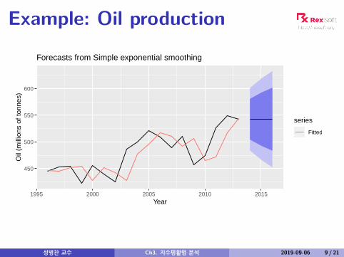
Example: Oil production
450
500
550
600
1995 2000 2005 2010 2015Year
Oil
(mill
ions
of t
onne
s)
series
Fitted
Forecasts from Simple exponential smoothing
성병찬 교수 Ch3. 지수평활법 분석 2019-09-06 9 / 21

Outline
1 Simple exponential smoothing
2 Trend methods
3 Seasonal methods
성병찬 교수 Ch3. 지수평활법 분석 2019-09-06 10 / 21
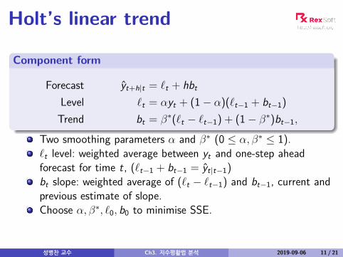
Holt’s linear trend
Component form
Forecast yt+h|t = `t + hbt
Level `t = αyt + (1− α)(`t−1 + bt−1)Trend bt = β∗(`t − `t−1) + (1− β∗)bt−1,
Two smoothing parameters α and β∗ (0 ≤ α, β∗ ≤ 1).`t level: weighted average between yt and one-step aheadforecast for time t, (`t−1 + bt−1 = yt|t−1)bt slope: weighted average of (`t − `t−1) and bt−1, current andprevious estimate of slope.Choose α, β∗, `0, b0 to minimise SSE.
성병찬 교수 Ch3. 지수평활법 분석 2019-09-06 11 / 21
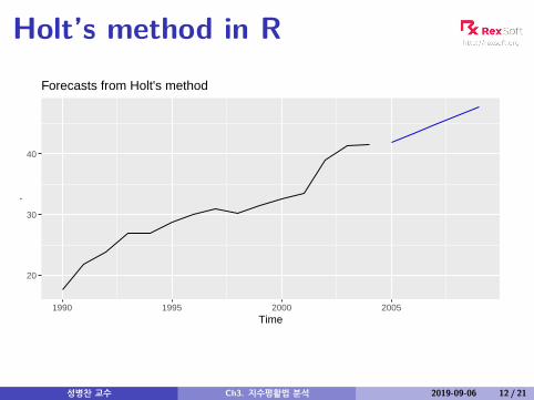
Holt’s method in R
20
30
40
1990 1995 2000 2005Time
.
Forecasts from Holt's method
성병찬 교수 Ch3. 지수평활법 분석 2019-09-06 12 / 21

Damped trend method
Component form
yt+h|t = `t + (φ+ φ2 + · · ·+ φh)bt
`t = αyt + (1− α)(`t−1 + φbt−1)bt = β∗(`t − `t−1) + (1− β∗)φbt−1.
Damping parameter 0 < φ < 1.If φ = 1, identical to Holt’s linear trend.As h→∞, yT+h|T → `T + φbT/(1− φ).Short-run forecasts trended, long-run forecastsconstant.
성병찬 교수 Ch3. 지수평활법 분석 2019-09-06 13 / 21
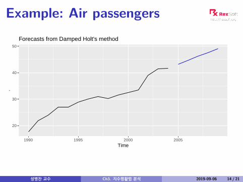
Example: Air passengers
20
30
40
50
1990 1995 2000 2005Time
.
Forecasts from Damped Holt's method
성병찬 교수 Ch3. 지수평활법 분석 2019-09-06 14 / 21
Outline
1 Simple exponential smoothing
2 Trend methods
3 Seasonal methods
성병찬 교수 Ch3. 지수평활법 분석 2019-09-06 15 / 21
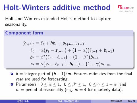
Holt-Winters additive methodHolt and Winters extended Holt’s method to captureseasonality.
Component form
yt+h|t = `t + hbt + st+h−m(k+1)
`t = α(yt − st−m) + (1− α)(`t−1 + bt−1)bt = β∗(`t − `t−1) + (1− β∗)bt−1
st = γ(yt − `t−1 − bt−1) + (1− γ)st−m,
k = integer part of (h − 1)/m. Ensures estimates from the finalyear are used for forecasting.Parameters: 0 ≤ α ≤ 1, 0 ≤ β∗ ≤ 1, 0 ≤ γ ≤ 1− α andm = period of seasonality (e.g. m = 4 for quarterly data).
성병찬 교수 Ch3. 지수평활법 분석 2019-09-06 16 / 21
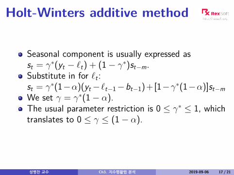
Holt-Winters additive method
Seasonal component is usually expressed asst = γ∗(yt − `t) + (1− γ∗)st−m.Substitute in for `t :st = γ∗(1−α)(yt−`t−1−bt−1)+[1−γ∗(1−α)]st−mWe set γ = γ∗(1− α).The usual parameter restriction is 0 ≤ γ∗ ≤ 1, whichtranslates to 0 ≤ γ ≤ (1− α).
성병찬 교수 Ch3. 지수평활법 분석 2019-09-06 17 / 21
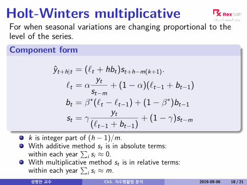
Holt-Winters multiplicativeFor when seasonal variations are changing proportional to thelevel of the series.Component form
yt+h|t = (`t + hbt)st+h−m(k+1).
`t = αyt
st−m+ (1− α)(`t−1 + bt−1)
bt = β∗(`t − `t−1) + (1− β∗)bt−1
st = γyt
(`t−1 + bt−1)+ (1− γ)st−m
k is integer part of (h − 1)/m.With additive method st is in absolute terms:within each year
∑i si ≈ 0.
With multiplicative method st is in relative terms:within each year
∑i si ≈ m.
성병찬 교수 Ch3. 지수평활법 분석 2019-09-06 18 / 21

Example: Visitor Nights
40
60
80
2008 2012 2016YearIn
tern
atio
nal v
isito
r ni
ght i
n A
ustr
alia
(m
illio
ns)
Data
HW additive forecasts
HW multiplicative forecasts
성병찬 교수 Ch3. 지수평활법 분석 2019-09-06 19 / 21

Estimated components
levelslope
season2007 2010 2013 2016
40
50
60
0.7008
0.7012
0.7016
−10−5
05
10
Year
Additive states
levelslope
season
2007 2010 2013 2016
40
50
60
0.65
0.70
0.75
0.80.91.01.11.2
Year
Multiplicative states
성병찬 교수 Ch3. 지수평활법 분석 2019-09-06 20 / 21
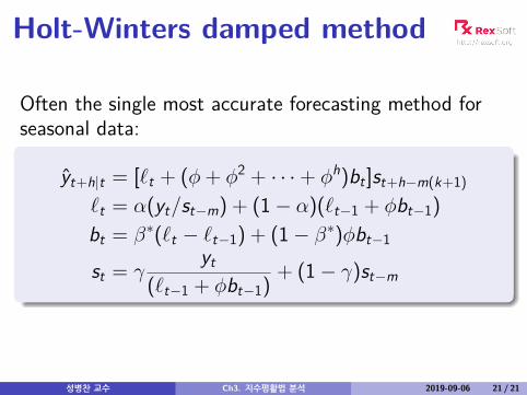
Holt-Winters damped method
Often the single most accurate forecasting method forseasonal data:
yt+h|t = [`t + (φ+ φ2 + · · ·+ φh)bt ]st+h−m(k+1)
`t = α(yt/st−m) + (1− α)(`t−1 + φbt−1)bt = β∗(`t − `t−1) + (1− β∗)φbt−1
st = γyt
(`t−1 + φbt−1)+ (1− γ)st−m
성병찬 교수 Ch3. 지수평활법 분석 2019-09-06 21 / 21
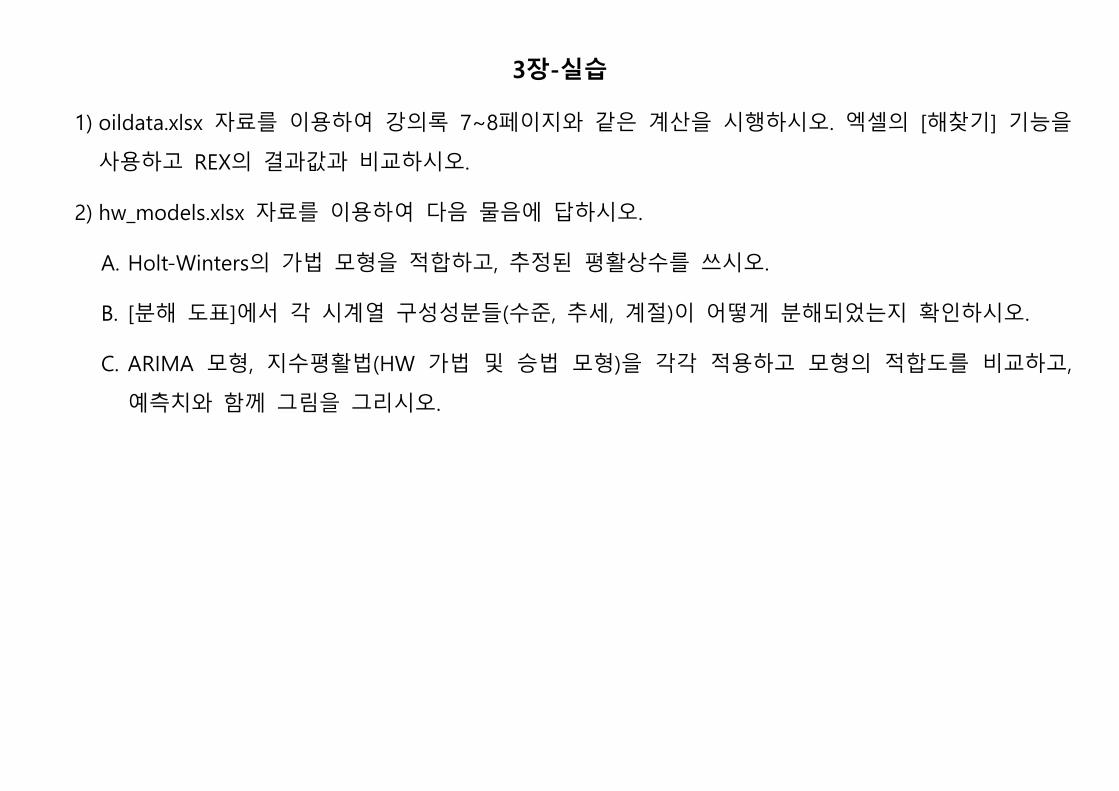
3장-실습
1) oildata.xlsx 자료를 이용하여 강의록 7~8페이지와 같은 계산을 시행하시오. 엑셀의 [해찾기] 기능을
사용하고 REX의 결과값과 비교하시오.
2) hw_models.xlsx 자료를 이용하여 다음 물음에 답하시오.
A. Holt-Winters의 가법 모형을 적합하고, 추정된 평활상수를 쓰시오.
B. [분해 도표]에서 각 시계열 구성성분들(수준, 추세, 계절)이 어떻게 분해되었는지 확인하시오.
C. ARIMA 모형, 지수평활법(HW 가법 및 승법 모형)을 각각 적용하고 모형의 적합도를 비교하고,
예측치와 함께 그림을 그리시오.


![Ó47 é4?4=-]'Î é { ã : ) f9 i1ú - n8^ ¹ ´ V / / + û é Ì Ç ü « £4È-ú ¤ / /1ñ æ ê / / Ç é t 1g %l æ Ê1ñ ½ æ%5 1ñ Ç" !¢ Ô Î é%51ñ é £! Ç ü « æ](https://static.fdocument.pub/doc/165x107/602daf6322287520c162e7e0/47-44-f-9-i1-n8-v-oe-4-.jpg)