CFD validation of hydrofoil performance characteristics in cavitating ...

CFD VALIDATION OF HYDROFOIL PERFORMANCE CHARACTERISTICS IN CAVITATING AND NON-CAVITATING FLOWS

Tristan L. Wood

B. Eng. Mechanical Engineering Project Report

Department of Mechanical Engineering Curtin University

2013

ii

[This page has been left intentionally blank]

iii

Mandurah WA 6210

08th November 2013

The Head Department of Mechanical Engineering, Curtin University, Kent Street, Bentley, WA 6102 Dear Sir: I submit this report entitled “CFD Validation of Hydrofoil Performance Characteristics in Cavitating and Non-Cavitating Flows”, based on Mechanical Project 491/493, undertaken by me as part-requirement for the degree of B.Eng. in Mechanical Engineering. Yours faithfully, Tristan L. Wood

iv


v

Acknowledgements

Foremost, I would like to express my sincere gratitude to my primary supervisor,

Doctor Andrew King for his continuous support of my final year project, for his

patience, enthusiasm and immense technical knowledge in the area of computational

fluid dynamics and the openFOAM open source CFD software, all of which have been

deeply appreciated.

I would similarly like to thank Doctor Tim Gourlay, Senior Research Fellow

with the Center for Marine Science and technology for his support and enthusiasm in

this project and his provision of data and technical materials used for the completion of

this project.

In addition I would like to acknowledge that this work was supported by Pawsey

funded iVEC through the use of advanced computing resources located at the

iVEC@murdoch facility by the use of their Epic HP Linux Cluster used to complete

CFD simulations that would have been impractical to achieve with standard computing

systems in the allotted time.

Finally I would like to thank my fellow Engineering Final Year students who

have provided both support and general advice for the duration of this project.

vi


vii

Abstract

This study attempts to validate the use of an open source CFD package, OpenFOAM to

assess the performance characteristics of a hydrofoil in both sub-cavitating and fully

cavitating flows and compare these to known performance characteristics for such a

design obtained previously using experimental methods. A symmetrical NACA 66-012

section hydrofoil was selected and its performance characteristics including parameters

such as lift and drag coefficients and quarter chord pitching moments were calculated

for a range of flow velocity’s and angles of attack in sub-cavitating flow and at a

constant angle of attack with varying cavitation numbers in cavitating flows, following

this the results were compared to the known data.

Results gained from the sub-cavitating simulations shows that the forces experienced on

a hydrofoil could be predicted to within a consistent 10-15% variance from the

experimental data published by Keerman in 1956. In the case of the cavitating flow

simulations showed large variances of up to 75% between the experimental and the

CFD data. Whilst this variance would be considered large for such work according to

work published by Gosset in 2010 notes that for a simulation using the OpenFOAM

solver model selected on a symmetrical hydrofoil that results within an order of

magnitude are acceptable.

Thus the knowledge gained from this study shows that the accuracy of the data gained

using CFD techniques to predict the performance characteristics of hydrofoils are highly

dependent on the complexity and design of modelling system used and the quantity of

computational processing power available.

viii

Nomenclature

1. ‘A’ Plan form area of hydrofoil (m2)

2. ‘α’ Hydrofoil angle of Attack (°)

3. ‘c’ Chord length of hydrofoil (m)

4. ‘CL’ Coefficient of Lift

5. ‘CD’ Coefficient of Drag

6. ‘CM’ Quarter Chord Pitching Moment

7. ‘CP’ Pressure Coefficient

8. ‘D’ Drag force on hydrofoil (N)

9. ‘η’ Performance ratio of hydrofoil

10. ‘g’ Acceleration due to gravity (m/s2)

11. ‘k’ Cavitation number

12. ‘L’ Lift force on hydrofoil (N)

13. ‘M’ Moment acting at quarter chord on hydrofoil (N.m)

14. ‘µ’ Dynamic Viscosity of water (N.s/m2)

15. ‘p’ Fluid Pressure (Pa)

16. ‘p∞’ Free stream fluid Pressure (Pa)

17. ‘pv’ Vapor pressure of fluid (Pa)

18. ‘Pr’ Prandtl Number

19. ‘Re’ Reynolds Number for fluid flows (Dimensionless Quantity)

20. ‘ρ’ Density of water in bed apparatus (kg/m3)

21. ‘q’ Dynamic Pressure (velocity Pressure) of flow (Pa)

22. ‘Sp’ Specific area of packing material (m2/m3)

23. ‘U’ Flow velocity of fluid in the bed apparatus (m/s)

24. ‘t ‘ Time component (s)

25. ‘τ’ Shear stress (Pa)

26. ‘u’ Velocity component in x axis (m/s)

27. ‘v’ Velocity component in y axis (m/s)

28. ‘ν’ Kinematic viscosity of fluid (m2/s)

29. ‘w’ Velocity component in z axis (m/s)

30. ‘x’ Spatial Ordinate

ix

31. ‘y’ Spatial Ordinate

32. ‘z’ Spatial Ordinate

Abbreviations

CFD - Computational Fluid Dynamics

RANS - Reynolds Averaged Navier-Stokes

LES - Large Eddy Simulation

DNS - Direct Numerical Simulation

NACA - National Advisory Committee on Aeronautics

STL - STereoLithography

VOF - Volume of Fluid

OpenFOAM - Open Field Operation And Manipulation

CAD - Computer Aided Design

FVM - Finite Volume Method

SST - Shear Stress Tensor

RMS - Root Mean Squared

x

Table of Contents

Page Number

1.0 Introduction ...................................................................................................................................... 1

1.1 Project Objectives .................................................................................................................. 6

1.2 Scope and Limitations of Theoretical Data Produced ........................................... 7

2.0 Background ........................................................................................................................................ 9

2.1 Theory ........................................................................................................................................ 9

2.1.1 Navier-‐Stakes Equations ....................................................................................... 9

2.1.2 Performance criteria of Hydrofoils ................................................................ 14

2.1.3 Cavitation Effects on Hydrofoils and Lifting Surfaces ............................ 16

2.1.4 Computational Fluid Dynamics ........................................................................ 22

2.1.5 Turbulence Modelling .......................................................................................... 26

2.1.6 Literature Review .................................................................................................. 29

3.0 Construction of SimpleFoam Sub-‐Cavitating Simulations ........................................... 31

3.1 Constructing NACA66-‐012 Hydrofoil Model and Flow Domain Meshing .. 31

3.2 Determining Field Constants and transport Properties .................................... 37

3.3 Simulation of Foil Performance in Sub-‐Cavitating Flows ................................. 39

3.4 Ensuring Data Extracted from Simulations is Valid for Use ............................ 40

3.5.1 Sub-‐Cavitating Results for Flow Velocity’s of 9.45 Meters per Second

...................................................................................................................................................................... 43

3.5.2 Sub-‐Cavitating Results for Flow Velocity’s of 12.55 Meters per

Second ....................................................................................................................................................... 48

3.5.3 Sub-‐Cavitating Results for Flow Velocity’s of 17.50 Meters per

Second ....................................................................................................................................................... 52

4.0 Simulation of NACA66-‐012 Foil in Cavitating Flow Conditions ................................ 57

5.0 Discussion ......................................................................................................................................... 63

6.0 Conclusions ...................................................................................................................................... 67

6.1 Recommendation for Future Works. ......................................................................... 68

7.0 References ........................................................................................................................................ 69

Appendices .............................................................................................................................................. 71

xi

List of Figures Page Number Figure 1: Fluid Element Subject to Forces According to Law of Conservation of

Mass ............................................................................................................................................................ 10

Figure 2: Diagram Depicting Forces Acting on Hydrofoil ................................................... 15

Figure 3: Modes of Heterogeneous Nucleation on Various Surface Conditions ........ 17

(Brennan 2003) ..................................................................................................................................... 17

Figure 4: Image of Hydrofoil Design From Dassault Systems Solidworks .................. 33

Figure 5: Image of STL of NACA 66-‐012 Hydrofoil ................................................................ 34

Figure 6: Diagram of NACA66-‐012 Foil in Flow Domain ..................................................... 35

Figure 7: Wire-‐Frame Diagram of Mesh Surrounding NACA66-‐012 foil at 5° Angle

of Attack .................................................................................................................................................... 36

Figure 8: Turbulent Kinetic Energy for Given Flow Velocities ......................................... 38

Figure 9: Specific Dissipation Rate for Given Flow Velocities .......................................... 38

Figure 10: Residual Plot for U = 9.45 m/s and α = 2° ............................................................ 40

Figure 11: Force coefficients for U = 9.45 m/s and α = 2° .................................................. 41

Figure 12: Velocity Field of NACA66-‐012 Foil at U =9.45 m/s and α = 13° ................. 43

Figure 13: Pressure Field of NACA66-‐012 Foil at U =9.45 m/s and α = 13° ............... 44

Figure 14: Pressure Across Top Side of NACA66-‐012 Foil at U =9.45 m/s and α =

13° ............................................................................................................................................................... 44

Figure 15: Pressure Across Under Side of NACA66-‐012 Foil at U =9.45 m/s and α =

13° ............................................................................................................................................................... 45

Figure 16: Comparison of Coefficients of Lift at U = 9.45 m/s .......................................... 45

Figure 17: Comparison of Coefficients of Drag at U = 9.45 m/s ....................................... 46

Figure 18: Comparison of Quarter Chord Pitching Moments at U = 9.45 m/s ........... 46

Figure 19: Performance Ratio of NACA66-‐012 Foil at U =9.45 m/s .............................. 47

Figure 20: Velocity Field of NACA66-‐012 Foil at U =12.55 m/s and α = 11° .............. 48

Figure 21: Pressure Field of NACA66-‐012 Foil at U =12.55 m/s and α = 11° ............ 49

Figure 22: Comparison of Coefficients of Lift at U = 12.55 m/s ....................................... 49

Figure 23: Comparison of Coefficients of Drag at U = 12.55 m/s .................................... 50

xii

Figure 24: Comparison of Quarter Chord Pitching Moments at U = 12.55 m/s ........ 50

Figure 25: Performance Ratio of NACA66-‐012 Foil at U =12.55 m/s ............................ 51

Figure 26: Velocity Field of NACA66-‐012 Foil at U =17.50 m/s and α = 5° ................. 52

Figure 27: Pressure Field of NACA66-‐012 Foil at U =17.50 m/s and α = 5° ............... 53

Figure 28: Comparison of Coefficients of Lift at U = 17.50 m/s ....................................... 53

Figure 29: Comparison of Coefficients of Drag at U = 17.50 m/s .................................... 54

Figure 30: Comparison of Quarter Chord Pitching Moments at U = 17.50 m/s ........ 54

Figure 31: Performance Ratio of NACA66-‐012 Foil at U =17.50 m/s ............................ 55

Figure 32: Close View Vapor Fraction at Cavitation Number k =1.518, U = 9.45 m/s

and α = 10° ............................................................................................................................................... 58

Figure 33: Vapor Fraction at Cavitation Number k =0.220, U = 9.45 m/s and α = 10°

...................................................................................................................................................................... 58

Figure 34: Velocity Magnitude Field at Cavitation Number k =1.518, U = 9.45 m/s

and α = 10° ............................................................................................................................................... 59

Figure 35: Pressure Magnitude Field at Cavitation Number k =1.518, U = 9.45 m/s

and α = 10° ............................................................................................................................................... 59

Figure 36: Comparison of Coefficients of Lift at U = 9.45 m/s and α = 10 ° ................ 60

Figure 37: Comparison of Coefficients of Drag at U = 9.45 m/s and α = 10 ° ............. 60

Figure 38: Comparison NACA66-‐012 Performance Ratios at U = 9.45 m/s and α =

10 ° .............................................................................................................................................................. 61

List of Tables Table 1: Design Geometry of NACA66-012 Hydrofoil………………………………..32

1

1.0 Introduction

The basic principle of standard hydrofoil craft is to raise a ships hull from the water and

support it dynamically on a wing like foil lifting surface. The effect of lifting a ships

hull from the water include the reduction of wave effects on the ship resulting in a

smother ride as well as a decrease in power required to maintain modestly high cruising

speeds as the hull no longer suffers drag effects from the water. Historically when

designing hydrofoil craft, engineers and marine architects have relied on empirical

methods and data for the selection of hydrofoil sections followed by costly and time

consuming experimental testing of scale and full sized models.

Currently hydrodynamic data is widely available for a large range of standardized

geometric shapes such as wedges, plates and circular arc hydrofoils as well as

conventional cambered airfoil shapes. Symmetrical hydrofoil shapes have traditionally

played important roles as both lifting surfaces and non-lifting support struts and fairings

as the requirements for such structures including drag profiles and strength requirements

are very similar to lifting hydrofoils.

Estimates place a theoretical weight limit of somewhere in the vicinity of 400 tones

displacement for practical designs of hydrofoil craft using current hydrofoil technology

(Pike, J. 2011). This limit is an application of the square-cube rule where the lift

generated by a hydrofoil is proportional to its planform area, whilst the weight that each

foil must support is proportional to volume or linear dimension cubed. Thus above this

limit the foils tend to outgrow the hull dimensions and result in a number of

impracticalities that render such designs unsuitable for commercial uses. In aircraft

design such a problem would be countered by increasing wing loading or operational

speeds, however in hydrofoil craft this is generally not an option as practical hydrofoil

speeds are limited by cavitation effects.

Thus to continue the development of heavier and higher speed hydrofoil craft new and

novel designs are required for hydrofoils that may include highly asymmetrical super-

2

cavitating or base vented foils or even multi component foils with variable geometries

for operating over a range of speeds.

The development of said advanced hydrofoil designs using traditional experimental

methods would be both time consuming and exorbitantly expensive, however by using

CFD techniques this process can be optimized to reduce both time and costs with

experimental testing required only at the final phase to confirm the performance

characteristics of a hydrofoil designed using these practices. Unfortunately as a result of

poor performance in the earlier years of development, naval architects and engineers

tend to express an inherent distrust in CFD and the data it provides. Due to this there is

a need for continual development of CFD techniques and technologies and for engineers

in this field to confirm that accurate data can be practically produced using such

methods.




design obtained previously using experimental methods.

To begin this project the first requirement was to select a foil design to test. The

selected foil for this project was a (National Advisory Committee on Aeronautics)

NACA66-012 profile foil. The reason for the selection of this foil was that it is a

symmetrical foil of a type commonly used for lifting bodies, control surfaces and

supporting struts also as most foils are only operated with angles of attack between 0

and 15 degrees selection of a symmetrical foil limits the number of simulations required

to understand the performance of the foil for each flow condition as performance will be

comparable with both positive and negative angles of attack. Additionally there was a

large quantity of data available on the performance characteristics of this foil in both

sub-cavitating flows and cavitating flows at a range of flow velocities and angles of

attack.

3

Design of the model of the foil was carried out using data from the National Advisory

Committee on Aeronautics database of foil designs and was modelled using Dassault

systems Soildworks to create a three dimensional model of the foil used by Keerman for

his experimental testing. Following this a STereoLithography model of the foil was

created from the Solidworks design. This model was created as this open source format

allows for the inbuilt meshing tools in OpenFOAM to create a mesh around the foil.

Following this a suitable domain was selected to both allow for modelling of effects

upstream of the foil and those downstream in the wake of the foil. With the model and

domain defined and the boundary conditions set simulations were carried out for sub

cavitating flow conditions using OpenFOAM’s simpleFoam solver for a range of flow

velocities ranging from 9.45 meters per second to 17.5 meters per second. For these

flows the foil was adjusted from angles of attack of 0 through to a maximum of +13

degrees in one-degree increments. SimpleFoam is a steady state solver inbuilt into

OpenFOAM for solving incompressible flows with turbulence modelling. Results for

lift and drag forces as well as quarter chord pitching moments were recorded and then

compared to those predicted by the experimental data published by Keerman.

Forces acting on the hydrofoil were obtained by integrating the pressure acting upon the

hydrofoil and then resolving the resultant force into forces in the directions normal and

parallel to the flow to determine the lift and drag forces. The coefficients of lift and drag

were the determined by Appling these forces to the lift and drag equations which

accounts for the free stream dynamic pressure and plan form area of the foil.

Simulation of the cavitating flow conditions were carried out in a similar manner to the

non-cavitating flow conditions with several exceptions. Rather than adjusting the flow

velocity and angle of attack a constant flow velocity of 9.45 meters per section and

angel of attack of 10 degrees were used and the cavitation number of the flow from a

range of 0.220 to 5.4 was adjusted by altering the free stream pressure of the fluid.

Additionally a multi-phase solver from OpenFOAM, inetrPhaseChangeFoam was used

in place of simpleFoam. This solver is a model based on solving for 2 incompressible,

4

isothermal immiscible fluids with phase-change (e.g. cavitation) using a VOF (volume

of fluid) phase-fraction based interface capturing approach. As in the sub-cavitating

case the forces acting on the foil were determined by integration of pressure and the

coefficients of lift and drag were calculated in the same manner. The resulting forces

were also compared to those predicted by Keerman and in addition the hydrofoil

performance ratios (ratio of lift to drag) were calculated and also compared.

Simulation of the sub-cavitating cases took approximately 70-80 CPU hours to

complete with the results showing an interesting series of trends. Analyses of the

determined coefficients of both lift and drag in the sub-cavitating case shows that the

simpleFoam model tends to over predict the forces acting on the hydrofoil. In all cases

the resultant forces were over predicted, usually by approximately 10% but in some

cases a number of points were as far as 25% above predicted results. However the

model also tended to over predict the drag forces by an amount greater than the lift

forces. This resulted in the hydrofoil performance ratio (lift to drag ratio) being

consistently less than what was predicted by Keerman.

Simulation of the cavitating flows was a much more computationally intensive process

requiring the use of iVEC’s supercomputing facilities to complete in a timely manner,

as each case required approximately 700-800 CPU hours to resolve. In this case the

results did not follow an obvious trend as was seen in the previous cases. For the lift

forces experienced by the foil the results obtained for cavitation numbers of 1.5 through

3.5 showed a reasonable level of agreement within what would have been expected for

such a simulation whilst at lover cavitation numbers the lift force produce was far

greater than what was experimentally determined and at higher cavitation numbers the

lift force calculated was slightly lower than experimental data predicted. The drag

forces experienced by the foil also tended to show a large variance between the

experimental and the computational results. For cavitation numbers between 1 and 3.3

the drag forces tended to be under predicted by between 50 and 75% and whilst outside

this set of cavitation numbers the reverse is the case with the forces tending to be over

predicted by as great a margin.

5

Whilst these variances would be considered quite large for experimental type work,

analysis covered in (Gosset 2010) where a very similar type simulation was attempted

shows that in the case of cavitating flows when using a solver such as

interphaseChangeFoam that results of coefficients of lift and drag within an order of

magnitude can be considered acceptable results.

There are a number of possible sources of error that could have contributed to the

variances between the experimental data and that from the CFD simulations. For the

sub-cavitating flows the use of the very basic simpleFoam solver model that does not

allow for compressibility of the fluid could have contributed to the error in the results.

Additionally turbulence modelling on the surface of the hydrofoil using the RANS two

equation k-ω SST model could have also contributed. Whist RANS turbulence

modelling is one of the least processor intensive model schemes it is known to produce

poor results in comparison to a more advanced turbulence model such as LES and is this

considered to be among “the best of the worst”.

In the case of the cavitating flow simulations there were also a number of possible

sources of error. Firstly cavitation is a complex phenomenon and there are a large

variation in methods for modelling its effects such as models based on barotropic

equations of state or like the model used base on the transport equation of vapour

fractions. The result of using different modelling methods is that some work only in

specific styles of simulations and thus the selection of the most suitable model is

important in producing accurate results. Additionally in order to save computational

power in already computationally intensive simulations turbulence was modelled using

a laminar model scheme, which could have also resulted in potential errors in the

results.

6

1.1 Project Objectives

There were a number of objectives for this project including

1. The first objective was to develop a working understanding of the open source

OpenFoam computational fluid dynamics software in the Ubuntu operating

environment then using this knowledge construct a series of CFD cases for

determining the performance characteristics of a NACA66-012 hydrofoil.

2. Determine the performance characteristics including coefficient of lift and drag as

well as the quarter chord pitching moments for NACA66-012 hydrofoil in sub-

cavitating flows for flow velocities ranging from 9.45m/s to 17.5 m/s and angles

of attack from 0-13°

3. Determine the performance characteristics including coefficient of lift and drag as

well as the quarter chord pitching moments for NACA66-012 hydrofoil in

incipient cavitation and fully developed cavitation flows for cavitation numbers

ranging from 0.220 to 5.337 for a flow velocity of 9.45 m/s and angle of attack of

10°

7

1.2 Scope and Limitations of Theoretical Data Produced

1. The simulation was designed to test the performance characteristics of a

NACA66-012 hydrofoil in a range of flow conditions and thus the hydrofoil

model has a constant cross section and no supporting structure that would be

required in real world applications of the foil and would therefore have

interacting effects on the flow around the foil.

2. For sub-cavitating flows the use of the basic simpleFoam solver does not allow

for compressibility or transient flows of the fluid in question. Whilst this is not a

problem as the simulations were steady state and water is very nearly

incompressible at the pressures in question, this solver is considered one of the

most basic models available in the OpenFOAM package and fails to account for

a number of fluid dynamics.

3. The Reynolds Averaged Navier Stokes (RANS) model used in the sub-

cavitating simulations will only produce the average of the turbulent flow at

each point rather than produce individual point data. This was used in order to

reduce processing costs at the expense of accuracy.

4. The use of a laminar turbulence scheme for the cavitating flow simulations

rather than a RANS scheme in order to save on processing power will result in a

loss of accuracy in these simulations.

5. The use of the constant cross sectional foil that terminates at the front and rear

boundary results in the flow effects that occur at the edge of the foil not being

accounted for in the simulation.

8

[This Page Has Been Left Intentionally Blank]

9

2.0 Background

2.1 Theory

2.1.1 Navier-Stakes Equations

The cornerstones of CFD are the fundamental governing equations of fluid dynamics

and are the continuity, momentum and energy equations. These equations are

mathematical expressions of the three physical principles on which all fluid dynamics

are based. To express these principles simply:

1. All mass, temperature and energy of a fluid are conserved

2. The momentum of each fluid particle is equal to the sum of the forces on a

particle according to Newton’s second law

3. The rate at which energy is gained or lost by the system or particle, shall

always equal the sum of the rate of heat flow and the rate of work done on that

system according to the first law of thermodynamics

Using the above three laws it is possie to describe the physical properties of a fluid

element using a Cartesian coordinate system. The Navier-Stokes equations are a series

of equations, which can be used to represent through mathematical expressions the

combined influence of external factors on individual fluid elements. These equations

were based on a Newtonian model of vicious stresses within a fluid medium and can be

defined in three time dependent dimensions using a series of five partial differential

equations.

Considering specifically at the conservation of mass for a finite element of fluid in a

given system the following conservation of mass diagram can be constructed.

10

Figure 1: Fluid Element Subject to Forces According to Law of Conservation of Mass

This above diagram defines exclusively the mass flow rates of fluid entering and exiting

the system without accounting for momentum changes and energy transfers involving

the system. Taking this above system and arranging all terms of the resulting mass

balance on the left hand side and dividing by the element volume δxδyδz yields.

𝜕𝜌𝜕𝑡 +

𝜕(𝜌𝑢)𝜕𝑥 +

𝜕(𝜌𝑣)𝜕𝑦 +

𝜕(𝜌𝑤)𝜕𝑧 = 0

Thus for a system utilizing an incompressible fluid with a fixed density such as that

utilised by OpenFOAM’s simpleFoam model the net mass flow rate of the element can

be defined by the following equation where:

𝜕𝑢𝜕𝑥 +

𝜕𝑣𝜕𝑥 +

𝜕𝑤𝜕𝑥 = 0

Stating the above equation plainly “the rate of increase of a property per unit mass of

fluid element and the net flow of the property per unit mass of fluid element are equal

ate of increase of a property per unit mass for a fluid particle”

11

For the same fluid element the conservation of momentum can be defined by the

flowing equation where:

𝜌𝛿𝑢𝛿𝑡 + 𝑢

𝛿𝑢𝛿𝑥 + 𝑣

𝛿𝑢𝛿𝑦 + 𝑤

𝛿𝑢𝛿𝑧 = 𝐶𝑜𝑛𝑠𝑡𝑎𝑛𝑡

The momentum equation in a specific Cartesian plane can be found by setting the rate

of change of the momentum of the fluid element in a Cartesian axis equal to the total

force in that axis on the element due to surface stresses plus the rate of increase of

momentum in that axis due to external sources yielding the following equations:

The x-component of the momentum equation:

𝜌𝐷𝑢𝐷𝑡 =

𝑑(−𝑝 + 𝜏!!)𝑑𝑥 +

𝑑𝜏!"𝑑𝑦 +

𝑑𝜏!"𝑑𝑧 + 𝑆!"

The y-component of the momentum equation:


𝑑(−𝑝 + 𝜏!!)𝑑𝑦 +

𝑑𝜏!"𝑑𝑥 +

𝑑𝜏!"𝑑𝑧 + 𝑆!"

The z-component of the momentum equation:


𝑑(−𝑝 + 𝜏!!)𝑑𝑧 +

𝑑𝜏!!𝑑𝑦 +

𝑑𝜏!"𝑑𝑥 + 𝑆!"

For Newtonian fluids the governing equations contain as further unknowns the viscous

stress components. In many fluid flows the viscous stresses acting on a fluid element

can be expressed as functions of local deformation rates. In three-dimensional flows the

local rate of deformation is composed of the linear deformation and volumetric

deformation rates. The rate of linear deformation of a fluid element has a total of nine

12

components in all three dimensions, six of which are fully independent when the fluid

in question exhibits isotropic behaviour (Schlichting, H 2000).

The three linear deformation components are defined by:

𝑠!! =!"!"

𝑠!! =!"!"

𝑠!! =!"!"

The six shearing linear deformation components are defined by:

𝑠!" = 𝑠!" =!!

!"!"+ !"

!" 𝑠!" = 𝑠!" =

!!

!"!"+ !"

!" 𝑠!" = 𝑠!" =

!!

!"!"+ !"

!"

The volumetric deformation of the fluid element is defined by:

𝑑𝑢𝑑𝑥 +

𝑑𝑣𝑑𝑦 +

𝑑𝑤𝑑𝑧 = 𝑑𝑖𝑣 𝒖

For a Newtonian fluid, the viscous stresses are proportional to the rates of deformation.

The three dimensional form of Newton’s law of viscosity for flows of compressible

fluids requires the use of two constants of proportionality. The first of these is the

dynamic viscosity, µ, which is used for the relation of stresses to linear deformations

and the second constant termed second viscosity, λ, used for the relation of stresses to

volumetric deformation.

These nine viscous stress components may be described by the following relationships

where:

𝜏!! = 2𝜇 !"!"+ 𝜆 𝑑𝑖𝑣 𝒖 𝜏!! = 2𝜇 !!

!"+ 𝜆 𝑑𝑖𝑣 𝒖 𝜏!! = 2𝜇 !"

!"+ 𝜆 𝑑𝑖𝑣 𝒖

𝜏!" = 𝜏!" = 𝜇 !"!"+ !"

!" 𝜏!" = 𝜏!" = 𝜇 !"

!"+ !"

!" 𝜏!" = 𝜏!" = 𝜇 !"

!"+ !"

!"

13

Substituting the above equations into the previously defined momentum equations

yields the three momentum partial differential equations of Navier-Stokes equations.

These equations were derived independently by English mathematician and physicist

George G. Stokes and French engineer Claude-Louis Navier in the early 1800s. Navier-

Stokes equations are in effect an extension of the previously defined Euler equations

and serve to include the effects of viscosity on fluid flows. These equations are a set of

five coupled differential equations that could in theory be solved using calculus

techniques and defined by:

𝜕𝜌𝜕𝑡 +

𝜕(𝜌𝑢)𝜕𝑥 +

𝜕(𝜌𝑣)𝜕𝑦 +

𝜕(𝜌𝑤)𝜕𝑧 = 0

!(!")!"

+ !(!!!)!"

+ !(!"#)!"

+ !(!"#)!"

= − !"!"+ !

!!!

!!!!!"

+ !!!"!"

+ !!!"!"

!(!")!"

+ !(!"#)!"

+ !(!!!)!"

+ !(!"#)!"

= − !"!"+ !

!!!

!!!"!"

+ !!!!!"

+ !!!"!"

!(!")!"

+ !(!"#)!"

+ !(!"#)!"

+ !(!!!)!"

= − !"!"+ !

!!!

!!!"!"

+ !!!"!"

+ !!!!!"

𝜕(𝐸!)𝜕𝑡 +

𝜕(𝑢𝐸!)𝜕𝑥 +

𝜕(𝑣𝐸!)𝜕𝑦 +

𝜕(𝑤𝐸!)𝜕𝑧

= −𝜕 𝑢𝑝𝜕𝑥 −

𝜕 𝑣𝑝𝜕𝑦 −

𝜕 𝑤𝑝𝜕𝑧 −

1𝑅𝑒! .𝑃𝑟!

𝜕𝑞!𝜕𝑥 +

𝜕𝑞!𝜕𝑦 +

𝜕𝑞!𝜕𝑧

+1𝑅𝑒!

𝜕𝜕𝑥 𝑢𝜏!! + 𝑣𝜏!" + 𝑤𝜏!" +

𝜕𝜕𝑦 𝑢𝜏!" + 𝑣𝜏!! + 𝑤𝜏!"

+𝜕𝜕𝑦 𝑢𝜏!" + 𝑣𝜏!" + 𝑤𝜏!!

14

2.1.2 Performance criteria of Hydrofoils

When determining the performance characteristics of a submerged body in a flow it is

best to define the acting forces with respect to a flow fixed coordinate system with the

origin at the midchord of the body (Jamieson, 1996). By integrating the pressure over

the surface of the body the resultant normal force acting on the lifting body can be

determined. Resolving this force into two components, one acting in the normal

direction to the flow and one acting in line with the flow termed lift L, and drag D,

forces respectively can be determined. Additionally a resultant moment M, will usually

exist around the origin for most lifting bodies, by general rule of thumb this moment is

taken to be positive when acting in the clockwise direction.

By taking these forces acting on the body a more useful performance criteria of a

submerged body can be defined by relating these forces to the density of the fluid, flow

velocity and a reference are for the body. These criterions are referred to as coefficients

of lift, drag and moment, these components result in non dimensional quantities by

dividing the forces and moment per unit span by the free stream dynamic pressure q,

and for hydrofoils the chord length c, where:

𝑞 =𝜌𝑈!!

2

𝐶! = !

!!!!

! ! 𝐶! =

!!!!

!

! ! 𝐶! = !

!!!!

! !

Note in the above equations the coefficients are based on a unit length of hydrofoil, thus

in the case of a hydrofoil of a specific width the chord value would be replaced by the

planform area A, defined as the multiple of the chord and span of the foil.

The hydrodynamic efficiency η, of a lifting body can be defined by the ratio of lift force

to drag force acting on a foil, where:

15

𝜂 = 𝐿𝐷 =

𝐶!𝐶!

As stated above the pitching moment on a foil is defined as the moment produced by the

hydrodynamic force on a foil if that force is applied not to the center of pressure but at

the aerodynamic center of the hydrofoil. It is worth noting that for symmetrical

hydrofoils both the center of pressure and aerodynamic center occur at approximately

25% of the chord from the leading edge. For a foil if the lift force is imagined to act

through the aerodynamic center the moment of the lift force changes in proportion to

the fluid velocity squared. If the moment is divided by the dynamic pressure, area and

chord of the foil the quarter chord pitching moment is defined. This value has

importance in the design of hydrofoils as it quantifies a portion of the total moment on

the foil that must be balanced. Thus the quarter chord pitching moment can be defined

by:

𝐶! = 𝑃𝑖𝑡𝑐ℎ𝑖𝑛𝑔 𝑀𝑜𝑚𝑒𝑛𝑡

𝜌𝑈!!2 𝐴. 𝑐

Figure 2: Diagram Depicting Forces Acting on Hydrofoil

16

2.1.3 Cavitation Effects on Hydrofoils and Lifting Surfaces

In a flow of liquid if the local pressure at a point falls below the vapor pressure of the

fluid a phase change from liquid to vapor is likely to occur. This phase change from

liquid to vapor due to this reduction in pressure is called cavitation. In order for this

phenomenon to occur there is an additional requirement to a drop in pressure, this

requirement is the inclusion of points of weakness in the form of small gas or vapor

inclusions operating as initiation sites for breakdown of the liquid. These microbubbles

within the fluid are termed cavitation nuclei and in the absence of such microbubbles it

is possible for liquids to withstand negative absolute pressures in much the same way as

solids. However in any practical application such weaknesses will occur in one of

several forms.

Firstly thermal motions within a fluid will form temporary microscopic voids that will

constitute the required nuclei necessary for rupture and growth of bubbles on a

macroscopic scale. This form of nucleation is termed homogeneous nucleation and

occurs spontaneously and randomly, without preferential nucleation sites. This form of

nucleation is of little importance in the investigation of cavitation effects on lifting

bodies.

The second form of nucleation is the more commonly observed manner that occurs

when major weaknesses occur at the boundary between a liquid and a solid wall or

small particles suspended within a liquid, where this happens with suspended particles it

is usually difficult to distinguish from homogeneous nucleation. When rupture occurs at

such sites it is termed heterogeneous nucleation, this form of nucleation is of much

more interest when studying cavitation effects.

Another form of cavitation nucleation occurs when micron sized bubbles of contaminate

gases, which may be attached to surfaces or within suspended particles or freely

suspended within the liquid. In the case of water microbubbles of air will persist almost

indefinitely and are almost impossible to remove outside of laboratory conditions. For

17

this reason the presence of such microbubbles tends to dominate most engineering

applications.

Figure 3: Modes of Heterogeneous Nucleation on Various Surface Conditions

(Brennan 2003)

As seen in the above figure displaying heterogeneous forms of cavitation nucleation

where contact angle between the vapor and solid intersection is denoted by θ. From this

the tensile strength T, of the bubble surface in the case of the flat hydrophobic surface

can be defined by:

𝑇 = 2𝑆.sin𝜃𝑅

Picture Removed for Copyright Reasons

18

From this theoretically the tensile strength would tend to zero, as 𝜃 → 𝜋 radians.

Alternatively the tensile strength on the hydrophilic surface is comparable with those of

homogeneous nucleation situations with much higher tensile strengths.

Of course surfaces on the scale relevant to the nucleation of cavitation are not flat

surfaces, so the effects of local geometry deformities must be considered (Brennan

2003). The case of the conical cavity in the above figure is often considered when

attempting to exemplify the affects of surface geometry. From this example if the half

angle of the vertex of such a cavity is denoted as α, then it is clear that a zero tensile

strength situation occurs at a much more realizable value of:

𝜃 = 𝛼 + 𝜋2

In addition should the value of 𝜃 be greater than defined in the above equation it is clear

that such a vapor bubble would grow and fill the cavity at pressures above the vapor

pressure for a liquid.

From this it is clear that surfaces will tend to have specific sites with optimum

geometry’s to promote nucleation of vapor bubbles and growth to macroscopic levels. It

is also clear that as local pressures are reduced further more sites will become capable

of generating and releasing vapor bubbles into the body of liquid.

The most common form of cavitation is though to occur in system where liquid flows

where hydrodynamic effects result in regions around surfaces where the local pressure

falls below vapor pressure of the fluid. The first person known to attempt to explain this

unusual behavior seen most commonly around ships propellers when operating at high

speeds in the later half of the 19th century was Osborne Reynolds who published a

number of papers on the field (Reynolds 1874). Reynolds mistake at the time was to

focus on the possibility of entrainment of air within the wake of the propeller blades, a

phenomenon currently understood as ventilation. Reynolds does not seem to have at any

19

point considered the possibility of the vaporization of liquid in propeller wakes. This

effect was not truly considered till work conducted by Parsons in 1906 when Froude

coined the term cavitation.

A Lifting surface such as a hydrofoil operating in a flow of liquid at sufficiently high

speed and angle of attack will be susceptible to the occurrence of cavitation. Cavitation

on such a hydrofoil will occur at the point of lowest pressure, which on most hydrofoil

designs will occur at the location of the suction peak just behind the leading edge of the

foil. Cavitation where it occurs on such lifting surfaces is usually considered

detrimental as it results in the loss of performance characteristics and causes flow

unsteadiness, leading to the generation of noise and vibration potential causing surface

erosion damage to the lifting body. Traditionally the design of hydrofoils has focused

on the complete elimination or if not possible then minimization of cavitation effects.

The extent to which cavitation occurs and the size of the cavitating region that develops

is dependent on a number of flow conditions and also the geometry of the foil. In order

to help clarify the level of cavitation occurring when discussing the phenomenon an

ultimately necessary, dimensionless but inadequate parameter of similitude was devised

to characterize such flows was determined based on the Euler number. This quantity

termed “cavitation number“ K, is defined by the following equation where:

𝐾 = 𝑃! − 𝑃!12𝜌𝑈!

!

In this equation the static pressure minus the vapor pressure for a given fluid is

compared as a ratio to the dynamic pressure. From this equation it is observed that

higher cavitation numbers will result in flows with less cavitation i.e. flows with a K

value greater than 3 are considered to have almost no cavitation potential and those with

very low cavitation numbers in the range of say 0.1 are considered to have a vey high

cavitation potential.

20

According to Franc and Michel (Franc, J., 2006) there are two distinct phases in the

development of cavitation experienced by submerged bodies. These two phases are

defined as:

• Phase 1: Cavitation inception, this phase describes a period of transition

between sub-cavitating flow regimen and a barely cavitating flow

regimen.

• Phase 2: Developed cavitation, this phase describes a form of cavitation,

which is maintained after nucleation by liquid vaporization effects, and

diffusion of non-condensable gasses across a clearly defined two phase

interface, in this case a cavity surface.

It is worth noting that a number of texts also include the existence of an additional

distinct phase occurring after the development of cavitation defined as super cavitation

(Savchenko 2001), where the dimensions of the cavity considerable exceed the

dimensions of the submerged body.

Cavitation nucleation as explained above is dependent on the presence of suitable

nucleation sites will originate at the location of the minimum value of the systems

pressure coefficient CPmin where:

−𝐶!"#$ ≥ 𝐾 = 𝑃 − 𝑃!12𝜌𝑈!

!

From this the quantity by which the minimum local pressure falls below the vapor

pressure can be termed the static delay to cavitation and is a function of the systems

nucleation conditions. In most practical engineering situations such a delay is so small

that it is standard procedure to take the following as an estimate for the cavitation

number at inception where:

21

𝐾! = −𝐶!"#$

Note that the negative sign in the above equation results from the definition of the

pressure coefficient where the local pressure is reduced below that of the free stream

pressure.

22

2.1.4 Computational Fluid Dynamics

Whist the Navier-Stokes equations were defined in the early 1800s their complexity

hindered their use in the solving of flows over complex geometries. In fact the earliest

numerical solution to a complex fluid dynamics problem of flow past a cylinder was not

published until 1933 and can be seen at (Thom A. 1933). Additionally one of the

earliest computed numerical solutions was produced by (Kawaguti M. 1953) involving

two-dimensional flow around a cylinder for a Reynolds number 40 flow using the full

Navier-Stokes equations. This process required Kawaguti to work 20 hours a week for

18 months using a desk calculator to solve.

Since this time numerous CFD modelling systems have been developed with the early

models generally consisting of in-house codes developed by corporations and were

specialised with purposes required by the corporation developing the code. The earliest

codes being two-dimensional models using the potential equations with very simple

vortex models. As computing power increased common models developed to the point

of using Euler equation based systems using turbulent flow models and increasingly

complex geometry’s. Modern CFD models are capable of using the full Navier stokes

equations for highly complex models with complex wake vortex and turbulence models.

Regardless of the modelling system or software package used all approaches follow a

similar procedure in the method of producing useable data.

The initial development of a CFD simulation is the pre-processing phase where the

system to be analysed is defined. This involves the following steps:

• The geometry or physical boundary of the system to be modelled is defined

• The volume of the system occupied by fluid is divided into discreet volumes or

cells, commonly referred to as a mesh.

• The physical modelling is defined, where the chosen equations of motion as well

as the physical interactions between fluids and surfaces are defined.

23

• Boundary conditions of the system are defined where the behaviour and

properties of the fluid at the boundaries such as the inlet and outlet as well as on

solid surfaces are defined.

With the development of easily accessible and open source CFD software in recent

years a number of third party tools have become available for the generation of meshes

rather than the use of the CFD software’s internal code allowing for much greater

manipulation of the mesh creation process. Additionally models are now much easier to

imported from a large number of computer aided design (CAD) software’s commonly

used by manufactures allowing for much more rapid development of CFD models.

Following this pre-processing phase the simulation of the system is started and the

equations of the chosen model are solved in an iterative process. Finally after the

simulation is completed a post processor is used to analyse and view the results of the

simulation and extract any relevant data.

Historically analysis of characteristics and performance of interactions between fluid

flows and surfaces has typically required the use of wind tunnel testing to determine

approximate values for system parameters and full scale model testing to provide

accurate and useable data. With the development of increasingly powerful computers

CFD has come to the forefront of tools used in the initial development of designs for

numerous manufacturing industries such as aerospace and naval architecture. Until

Recently simulations of the more exotic phenomenon such as cavitating flow and other

effects were limited to the self-developed "in house" CFD codes. With the introduction

of flexible open source software such as OpenFOAM (Open Source Field Operation and

Manipulation) the tools to analyse complex flows are now available to academic

institutions without the large capital expenditure that might otherwise be required to

purchase or develop a software package.

Whilst modern software packages perform with generally acceptable levels of accuracy

for most applications this was not so with the earlier versions of CFD software. Due to

24

these early inaccuracies modern industry has a tendency to mistrust data obtained from

CFD techniques discarding it as inaccurate and unreliable, preferring to rely on

empirical models developed through mass trials of physical models. This mistrust has

resulted in a drive to improve CFD techniques to improve the accuracy of the software

with respect to the data gained from empirical methods.

OpenFOAM is a free and open source CFD toolbox and software package produced by

OpenCFD Ltd and has a user base of both commercial and academic organisations

across a range of both engineering and science based disciplines. This software package

is highly developed and includes the capabilities to solve complex flow simulations

involving a range of circumstances including chemical reactions, complex turbulence

models and heat transfer. This software also includes pre-processing tools such as a

meshing tool capable of meshing complex CAD geometry’s but does not allow for easy

creation of complex geometry’s requiring third party CAD software for their generation.

The capabilities of the included solvers in the software range from simple models of

incompressible flows to compressible and multi-phase flow simulations as well as

buoyancy driven flows among others with a selection of 80 specialised solvers.

OpenFOAM also provides a selection of turbulence models including the Reynolds

averaged Navier-Stokes (RANS) and large eddy simulation (LES) methods.

Additionally the incorporated SnappyHexMesh mesh generation tool provides the

ability to generate highly detailed and customisable meshes around complex

geometry’s, however the software is also capable of accepting meshes generated from a

range of third party meshing tools such as Netgen, Gmesh and Blender.

When simulating fluid flows OpenFOAM has a suite of numerical tools used to solve a

range of problems. This includes methods of solving problems where matter is

represented both as a continuum and as discreet particles. When solving equations based

on a fluid continuum OpenFOAM uses a finite volume method (FVM) where matrix

equations are constructed using the FVM applied to arbitrary shaped cells. Additionally

a segregated, iterative solution is used where the governing equations of the system are

25

reduced to separate matrix equations created for each individual equation and are solved

within an iterative sequence. Also equation coupling is used where coupling between

related properties such as pressure and velocity are performed using adapted versions of

well-known algorithms such as PISO.

26

2.1.5 Turbulence Modelling

Turbulence is a key issue in most engineering applications of CFD techniques. This is a

result of nearly all engineering problems having some form of inherent turbulence and

thus requiring a method of turbulence modeling.

Turbulence is best defined as a state of motion of a fluid best defined as by what

appears to be random and chaotic vorticity. In situations where turbulence is present it

has a tendency to dominate all other flow characteristics, usually resulting in increased

energy dissipation, fluid mixing, heat transfer and drag effects on submerged bodies.

Modeling of real turbulence requires that it be done in three dimensions; this is a result

of the requirement of the ability of turbulence to create new vorticity from existing

turbulence. This is something that can only occur when the necessary stretching and

turning in three dimensions can be modeled.

For modeling turbulence there are a number of systems available with the most common

methods including models based on the Large Eddy Simulation (LES) scheme, the

Reynolds Averaged Navier-Stokes (RANS) Model and Direct Numerical Simulation

(DNS) scheme.

Of the above three methods DNS is considered to be the most accurate modeling

method for CFD simulations, this is as a result of this methods solving of each point

along the surface of a flow field. The disadvantage of such a method is that it requires

excessive processing power and extended periods of time to both implement and run.

For tis reason such a method is seldom used except in the case of where extreme

accuracy is required and both time and a suitable computing resource are available.

The principle behind the operation of LES simulation is the utilization of low pass

filtering. This technique is applied to the Navier-Stokes equations to eliminate

turbulence effects on smaller scales within the system. The consequence of this filtering

technique is a reduction on the processing power required to complete the simulation.

27

The effect of using LES simulation is the resolving of large scales of floe field solutions

with better fidelity that that offered by RANS techniques in addition it also models the

smallest and most computationally dependent scales rather than resolving them using

the extremely costly DNS method. This method allows for turbulent flow fields around

complex geometry’s being resolved with reasonable accuracies using supercomputing

resources.

The RANS method for turbulence modeling is one of the more common methods for

simulating turbulence in fluid flows. Whilst there are a large number of varied RANS

models the basic operating principle is shared among all, this principle being the

objective of computing the Reynolds stresses using one of three methods. These three

methods are the liner eddy viscosity mode, non-linear eddy viscosity model and the

Reynolds stress model.

In this project a RANS two-equation model is used where turbulence needs to be

considered. The selected model is the RANS k-ω SST, which includes two extra

transport equations to represent the turbulence of the fluid. The first included transport

variable is the turbulent kinetic energy k, and the second is the specific dissipation ω. In

this system k determines the energy in the turbulence whilst ω determines the scale of

the turbulence. This two-equation model allows for the accounting of historical effects

such as convection and the diffusion of turbulent energy. The reason for the selection of

this model for simulations is that it provides a good all-round turbulence model without

requiring an excess of additional processing power. This is a result of the model

combining the best aspects of both eddy and viscosity modeling techniques. The use of

the k omega formulation in the inner sections of the boundary layer makes said model

directly usable all the way through to the vicious sub layer. The SST component also

allows for switching to a k-epsilon behavior in the free stream avoiding a common k-

omega problem where the model tends to be too sensitive or free stream turbulence

properties. However it should be noted that the accuracy of RANS turbulence modeling

is considered to be somewhat dubious exemplified by (Spalart 2000) where it is stated

28

that RANS models of any complexity have “no reasonable claim” to provide accurate

stresses in complex flows.

Accurate representation of the total kinetic energy k, as a boundary condition when

using CFD techniques is important if the flow is to be accurately predicted. This is even

more so in the simulation of high Reynolds number flows where such turbulence may

have greater effect. The value for TKE may be calculated using the following equation

where:

𝑘 = 32 (𝑈𝐼)

!

Where I is the Initial turbulence intensity as a percent and can be defined by:

𝐼 = 0.16 𝑅𝑒!!/!

The specific turbulence dissipation rate ω, is defined as the rate at which TKE is

converted into thermal internal energy per unit volume and time where;

𝜔 = 𝜖𝑘𝛽

Where β is a model constant (β = 0.09) and ε is the turbulence dissipation described by:

𝜖 = 𝛽 𝑘!!

𝑙

Where l is the turbulence length scale is not a well-defined quantity and for most

situations is best set at approximately 5% of the channel height or hydraulic diameter

etc. This has the effect of ensuring that the turbulence length scale does not exceed the

size of the problem resulting in turbulent eddies far larger than would ever be expected.

29

2.1.6 Literature Review

Empirical data is available for a range of hydrofoil designs derived through

experimental methods. Force coefficients such as lift and drag ratios have been obtained

for a large number of shapes including simple geometric designs such as wedges,

circular cross sections and flat plates as well as more geometrically complex shapes

such as air and hydrofoils. Symmetrical hydrofoil shapes such as those described by

(Keerman R. 1956) serve important functions on many watercraft as both lifting

surfaces as well as support struts and non load bearing fairings an a range of structures.

These designs meet the general requirements for such an application; as they are easy to

design with a low drag, low critical cavitation number and high strength.

These characteristics of symmetrical cross section hydrofoils are agreed with in the

wartime report (Land, Norman S. 1943) where his investigation shoved that such a

hydrofoil (in this case a NACA 66 s-209) is capable of producing a high lift to drag

ratio at speeds that would be considered reasonable for modern watercraft and displayed

a low critical cavitation number, able to resist serious cavitation effects at to an angle of

12 degrees at a speed of 40 meters per second.

Cavitation is one of the most important effects suffered by hydrofoils. This

phenomenon occurs when the local pressure drops below the fluids vapour pressure

causing a change in phase. This effect can cause considerable damage to solid surfaces

and can also have dramatic effects on the performance of submerged bodies. For this

reason the effects of cavitation on hydrofoils have been an area of interest for CFD

researchers. Research conducted by (Shen Huang et al. 2010) into the modelling of a

NACA 66 type hydrofoil using Fluent CFD software to model steady cavitating flow at

a range of angle of attacks and cavitation numbers shows that CFD software is capable

of providing a good estimation of the effect on a hydrofoil at such conditions. Although

their results did show that at sections where the flow separated from the foil that the

CFD software did show variance to the experimental results outside what could be

considered normal experimental variation.

30

Investigation using numerical methods on 2D hydrofoils on cavitating flows was also

carried out by (Greeshma P. R. et al. 2012). This simulation was carried out on a non

standard symmetrical hydrofoil at an angle o attack of seven degrees at cavitation

numbers ranging from 2.5 to 4. This research showed that for this particular foil and

orientation incipient cavitation deployed at an approximate cavitation number of 3 to

3.5 and evolves to full unsteady cavitation around a cavitation number of 4, with super

cavitation conditions being met on further increase of the cavitation number. Also from

this model it was determined that as the cavitation effects occur that lift decreases and

drag increases.

Unsteady turbulent cavitation effects on a NACA-0015 section hydrofoil was studied by

(Kim, Sung-Eun. 2009) using the OpenFOAM toolkit. This simulation used a multi

phase solver with a liquid vapor mix modeled as an interpenetrating continuum with

hybrid RANS/LES turbulence model. The results gained from this simulation for the lift

and drag coefficients in a range of cavitation numbers were found to be in good

agreement with the experimental data for this hydrofoil in respect to mean values, root

mean squared values and spectral contents.

Simulation of cavitating flows on a symmetrical section hydrofoil using OpenFOAM’s

interPhaseChangeFoam was carried out in (Gosset 2010). Results from this research

showed that attempting to model cavitation effects on a foil using cavitatingFoam

produced highly unreliable results that did nor reflect real world cavity dynamics where

using interPhaseChangeFoam still produced unreliable results (better than

cavitatingFoam) but tended to better reflect real world cavitation dynamics. The

conclusions drawn by Gosset is attempting to model such a situation as this for

extracting hydrofoil performance characteristics using OpenFOAM is that results within

an order of magnitude to experimental results are of an acceptable nature.

31

3.0 Construction of SimpleFoam Sub-Cavitating Simulations

3.1 Constructing NACA66-012 Hydrofoil Model and Flow Domain Meshing

As stated above a NACA66-012 hydrofoil model was selected for testing as data was

found to be available for this hydrofoil in a wide range of flow conditions. As with most

standardized hydrofoil design geometry data for the foil is defined as stations and

ordinates as percent of the chord. In this case station refers to the percentage of chord

from the leading edge of the foil and ordinate the normal distance from the chord line to

the surface of the foil.

32

Table 1: Design Geometry of NACA66-012 Hydrofoil

NACA Profile 66-012 (Stations and ordinates given as per cent of airfoil chord)

x y dy/dx 0.0000 0.0000 N/A 0.5000 0.9038 0.8364 0.7500 1.0859 0.6399 1.2500 1.3525 0.4534 2.5000 1.8067 0.3142 5.0000 2.4936 0.2428 7.5000 3.0378 0.1968

10.0000 3.4933 0.1696 15.0000 4.2340 0.1292 20.0000 4.7996 0.0991 25.0000 5.2364 0.0763 30.0000 5.5656 0.0560 35.0000 5.7987 0.0376 40.0000 5.9424 0.0197 45.0000 5.9981 0.0022 50.0000 5.9642 -0.0163 55.0000 5.8339 -0.0366 60.0000 5.5857 -0.0659 65.0000 5.1477 -0.1097 70.0000 4.5122 -0.1398 75.0000 3.7677 -0.1571 80.0000 2.9432 -0.1706 85.0000 2.0807 -0.1723 90.0000 1.2346 -0.1643 95.0000 0.4738 -0.1352

100.0000 0.0000 -0.0016 L.E. radius = 0.870 percent chord

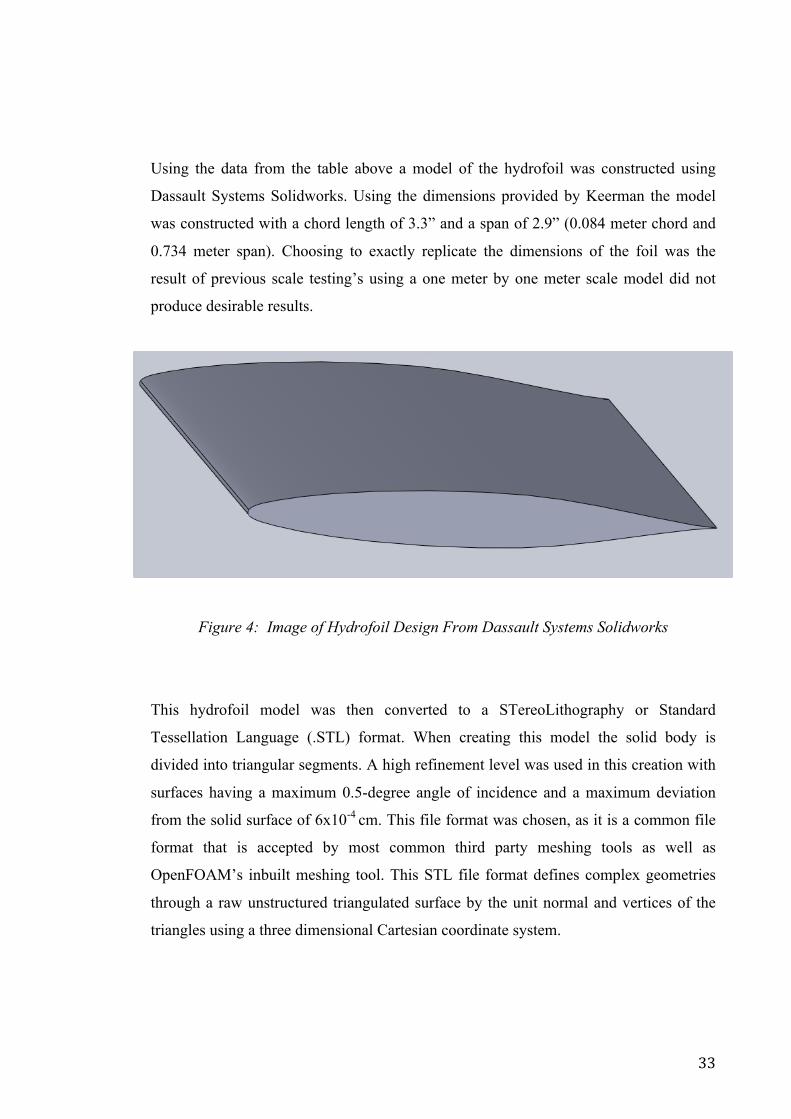
33

Using the data from the table above a model of the hydrofoil was constructed using

Dassault Systems Solidworks. Using the dimensions provided by Keerman the model

was constructed with a chord length of 3.3” and a span of 2.9” (0.084 meter chord and

0.734 meter span). Choosing to exactly replicate the dimensions of the foil was the

result of previous scale testing’s using a one meter by one meter scale model did not

produce desirable results.

Figure 4: Image of Hydrofoil Design From Dassault Systems Solidworks

This hydrofoil model was then converted to a STereoLithography or Standard

Tessellation Language (.STL) format. When creating this model the solid body is

divided into triangular segments. A high refinement level was used in this creation with

surfaces having a maximum 0.5-degree angle of incidence and a maximum deviation

from the solid surface of 6x10-4 cm. This file format was chosen, as it is a common file

format that is accepted by most common third party meshing tools as well as

OpenFOAM’s inbuilt meshing tool. This STL file format defines complex geometries

through a raw unstructured triangulated surface by the unit normal and vertices of the

triangles using a three dimensional Cartesian coordinate system.

34

Figure 5: Image of STL of NACA 66-012 Hydrofoil

The created STL file of the Hydrofoil consists of 1796 individual triangular sections.

Whilst theoretically able to handle both ASCII and binary formats when using this file

with both Netgen and snappyHexMesh the binary format appears to fail to mesh with a

consistent level of accuracy thus ASCII is the preferred format for this file.

When constructing the flow domain it was important to select a domain size great

enough to model all the effects occurring both in front of the hydrofoil and behind but

not so great as to increase the amount of computational power required extending the

required time to run the simulation. In order to best accommodate these requirements a

domain of 10 chord lengths long (parallel to flow vector) and 3.25 chord lengths high

(normal to flow vector) and 1 foil span wide was chosen with the center of rotation of

the hydrofoil placed 3 chord lengths from the inlet boundary and centered on the

vertical axis.

35

Figure 6: Diagram of NACA66-012 Foil in Flow Domain

Using the inbuilt snappyHexMesh function within OpenFOAM the foil was meshed

into the flow domain at the beginning of each simulation. Using a level (5,6) refinement

with 3 additional boundary layers and a refinement box surrounding the foil a mesh was

created that has a relatively coarse structure at distance from the hydrofoil and

increasing density as the distance to the foil decreases. This allows for an approximate

model of fluid as it moves away from the foil whilst attempting to model accurately

flow close to the foil. This resulted in a mesh of approximately 5.6 million cells varying

slightly when changing the angle of attack of the foil and re-meshing.

Prior to the selection of snappyHexMesh as the meshing tool to be used, other meshing

tools such as Gmesh and Netgen were trialed but failed to provide adequate and

repeatable results when importing into OpenFOAM. Thus due to the instability and

variance in meshes that were created these meshing tools were discarded as potential

options and it was decided to use the inbuilt tools.

36

Figure 7: Wire-Frame Diagram of Mesh Surrounding NACA66-012 foil at 5° Angle of

Attack

37

3.2 Determining Field Constants and transport Properties

Before running each simulation there are a number of transport properties and variables

that need to be calculated and input into the appropriate files in the OpenFOAM case

directory. These variables include the kinematic viscosity of the fluid, the turbulence

kinetic energy and the specific diffusion rate.

As the Reynolds number is provided for each flow velocity and angle of attack the

kinematic viscosity needs to be adjusted slightly for each simulation where:

𝑅𝑒 = 𝑉. 𝑐𝜈

Whilst this generally resulted in a change of less than a couple of percent from the

standardized value of 1 ×10!! 𝑚!/𝑠 used for water at approximately room temperature

it did eliminate this as a possible source of deviation between theoretical and

experimental results.

Additionally the turbulence kinetic energy k, and specific dissipation rate ω, needed to

be calculated for each flow velocity used, as both are a velocity dependent term. Values

for each are displayed in the following charts. Where they are calculated using:

𝑘 = 32 (𝑈𝐼)

!

and

𝜔 = 𝜖𝑘𝛽

38

Figure 8: Turbulent Kinetic Energy for Given Flow Velocities

Figure 9: Specific Dissipation Rate for Given Flow Velocities

0

0.05

0.1

0.15

0.2

0.25

0.3

0.35

0.4

0 2 4 6 8 10 12 14 16 18 20

Turbulent kinetic Energy k

Flow Velocity U m/s

0

0.2

0.4

0.6

0.8

1

1.2

1.4

0 2 4 6 8 10 12 14 16 18 20

SpeciDic Dissipation Rate (omega)

Flow Velocity U m/s

39

3.3 Simulation of Foil Performance in Sub-Cavitating Flows

Following the construction of the case files each simulation was run for the given angles

of attack and speed. The simulations were run for 800 seconds in half-second time steps

and the results recorded for intervals of every 12.5 seconds. Such a long time period for

the simulation was set as to ensure that for those flows at higher speeds and angles of

attack would have greater time to reach convergence and those that only reach a quasi

static state would produce enough data to calculate average performance characteristics.

However during to the relatively large number of cell used in the simulation a number

of preprocessing steps needed to be completed prior to running. Firstly using the

parDecompose function the domain was divided into a number of sections and each

section assigned to a computer processor for operation and on the completion of the

simulation the subdivisions were recombined into a single field. Additionally to reduce

the time required to convergence the potentialFoam function was run to initialize a

potential field across the domain and reduce overall running time by ensuring the flow

was partially resolved before the simulation started.

During the simulation a number of post processors were set to produce data. Among

these processors were two scripts designed to produce a log of the forces acting on the

hydrofoil in each Cartesian axis and a second script designed to calculate coefficients of

lift and drag from these forces as well as calculate the pitching moment of the hydrofoil.

40

3.4 Ensuring Data Extracted from Simulations is Valid for Use

For stead state and quasi-steady state solutions there are three conditions that need to be

met in order for there to be reasonable confidence in the data that is produced. When

looking for convergence in solutions the most common mistake made is to only

consider the values of the residuals, however in reality to be truly sure of convergence

values of points of interest should also be monitored and it should be ensured that the

domain has an imbalance of less than 1%.

Residuals of the flow are defined, as the difference between the actual values and the

values produced by the software package, thus are essentially the recording error for the

data. For each simulation the residual values for each velocity axis as well as pressure,

turbulent kinetic energy and specific dissipation rate were monitored. It was intended

for the simulation to be valid that the residuals meet a point where there is no oscillation

or variance or that the RMS value of each residual should not exceed a value of between

10-4 and 10-5.

Figure 10: Residual Plot for U = 9.45 m/s and α = 2°

41

Note looking at this plot of residuals above it is apparent strictly from this data that the

residuals would have been in a valid range by around the 800 time step mark however

running for the additional 800 time steps has produced slightly better results.

Additionally it is valid to run the simulations for such a long period as higher angles of

attack and velocities will take longer to meet convergence. Additionally in this plot the

residuals for the velocity in the y-axis appear to be several orders of magnitude greater

than all other values. This is an inherent property of the design of the simulation where

there is near no flow in the y direction resulting in there being large cumulative

recording errors for such data.

As stated above monitoring points of interest to observe the occurrence of having

reached a steady state solution is an important part of verifying convergence. For the

simulations both the coefficients of lift and drag were closely monitored throughout the

simulation.

Figure 11: Force coefficients for U = 9.45 m/s and α = 2°

-‐0.05

0

0.05

0.1

0.15

0.2

0.25

0.3

0.5 5 50 500

Force CoefDicient

Time Step

COEFICIENT OF LIFT

COEFICIENT OF DRAG

42

Note in this chart that the x-axis scale is logarithmic to emphasize the oscillations

towards the beginning of the simulation. Also worth noting that whist the coefficient of

drag reaches steady state within 20 time steps, whilst it is nearly 500 time steps before

the coefficient of lift reaches a stead situation.

Finally domain balancing was not considered as a tool for verifying convergence in

these simulations as it was unable to be determined if a tool for assessing this parameter

was available in the OpenFoam software package.

43

3.5.1 Sub-Cavitating Results for Flow Velocity’s of 9.45 Meters per Second

The first series of simulations were run at a flow velocity of 9.45 m/s at positive angles

of attack ranging from 0° through to 13° at 1° increments. These simulations were run

using OpenFOAM’s simpleFoam solver model. This solver utilizes an incompressible

stead state model with included turbulence modeling. Following this the foil was tested

at random negative angles of attack in the same manner as the experimental data to

prove the foils symmetrical nature. From these simulations coefficients for lift as well

as drag and quarter chord pitching moments were extracted. To obtain these

performance criteria pressure was integrated along the surface of the hydrofoil and the

resulting vector split into components and substituted into the equations defined in the

background theory. These results were then compared to experimental results from

(Keerman 1956).

Figure 12: Velocity Field of NACA66-012 Foil at U =9.45 m/s and α = 13°

44

Figure 13: Pressure Field of NACA66-012 Foil at U =9.45 m/s and α = 13°

Figure 14: Pressure Across Top Side of NACA66-012 Foil at U =9.45 m/s and α = 13°

-‐250

-‐200

-‐150

-‐100

-‐50

0 0 10 20 30 40 50 60 70 80 90 100

Hydrofoil Surface Local Pressure (kPa)

Hydrofoil Chord Percentage

45

Figure 15: Pressure Across Under Side of NACA66-012 Foil at U =9.45 m/s and α =

13°

Figure 16: Comparison of Coefficients of Lift at U = 9.45 m/s

-‐0.1

0

0.1

0.2

0.3

0.4

0.5

0.6

0.7

0.8

0.9

1

0 2 4 6 8 10 12 14

CoefDicient of Lift

Angle of Attack (a)

Experimental

CFD

-‐120

-‐100

-‐80

-‐60

-‐40

-‐20

0

20

40

60

0 10 20 30 40 50 60 70 80 90 100

Hydrofoil Surface Local Pressure (kPa)

Hydrofoil Chord Percentage

46

Figure 17: Comparison of Coefficients of Drag at U = 9.45 m/s

Figure 18: Comparison of Quarter Chord Pitching Moments at U = 9.45 m/s

0

0.05

0.1

0.15

0.2

0.25

0 2 4 6 8 10 12 14

CoefDicient of Drag

Angle of Attack (a)

Experimental

CFD

-‐0.06

-‐0.04

-‐0.02

0

0.02

0.04

0.06

0 2 4 6 8 10 12 14

Quarter Chord Pitching Mom

ent

Angle of Attack (a)

Experimental

CFD

47

Figure 19: Performance Ratio of NACA66-012 Foil at U =9.45 m/s

-‐10

0

10

20

30

40

50

0 2 4 6 8 10 12 14

Hydrofoil Performance Ratio

Angle of Attack (a)

Experimental

CFD

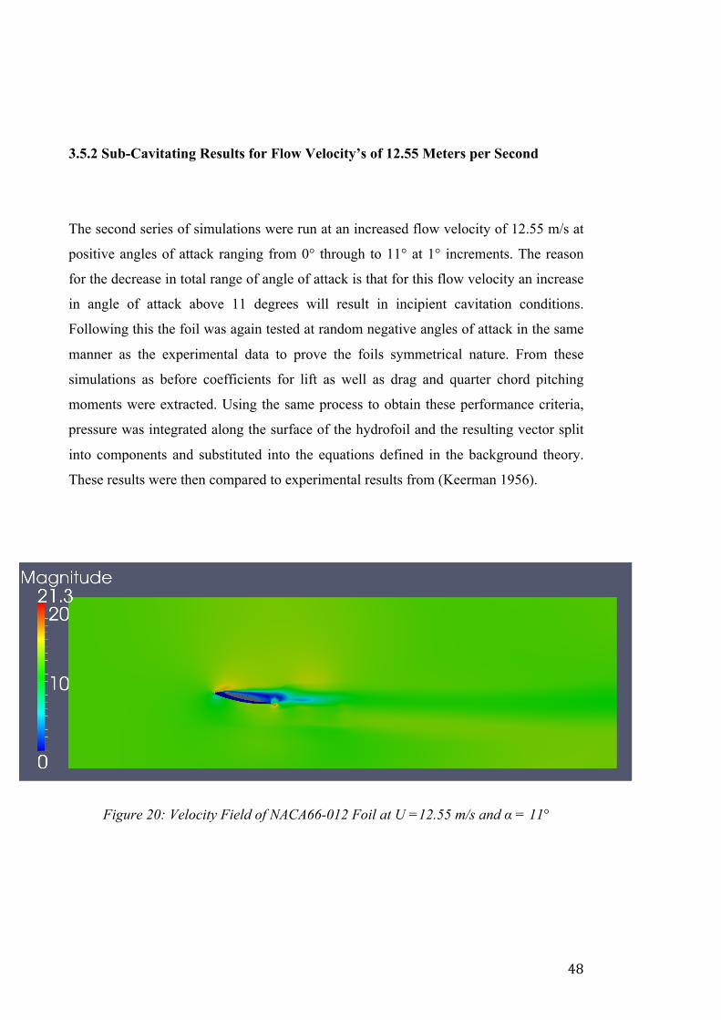
48


The second series of simulations were run at an increased flow velocity of 12.55 m/s at

positive angles of attack ranging from 0° through to 11° at 1° increments. The reason

for the decrease in total range of angle of attack is that for this flow velocity an increase

in angle of attack above 11 degrees will result in incipient cavitation conditions.

Following this the foil was again tested at random negative angles of attack in the same

manner as the experimental data to prove the foils symmetrical nature. From these

simulations as before coefficients for lift as well as drag and quarter chord pitching

moments were extracted. Using the same process to obtain these performance criteria,

pressure was integrated along the surface of the hydrofoil and the resulting vector split

into components and substituted into the equations defined in the background theory.

These results were then compared to experimental results from (Keerman 1956).


49



-‐0.1

0

0.1

0.2

0.3

0.4

0.5

0.6

0.7

0.8

0.9

0 2 4 6 8 10 12

CoeDicient of Lift

Angle of attack (a)

Experimental

SimpleFOAM

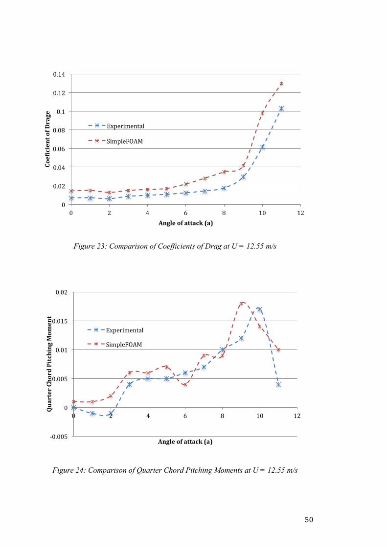
50



0

0.02

0.04

0.06

0.08

0.1

0.12

0.14

0 2 4 6 8 10 12

CoeDicient of Drage

Angle of attack (a)

Experimental

SimpleFOAM

-‐0.005

0

0.005

0.01

0.015

0.02

0 2 4 6 8 10 12

Quarter Chord Pitching Mom

ent

Angle of attack (a)

Experimental

SimpleFOAM

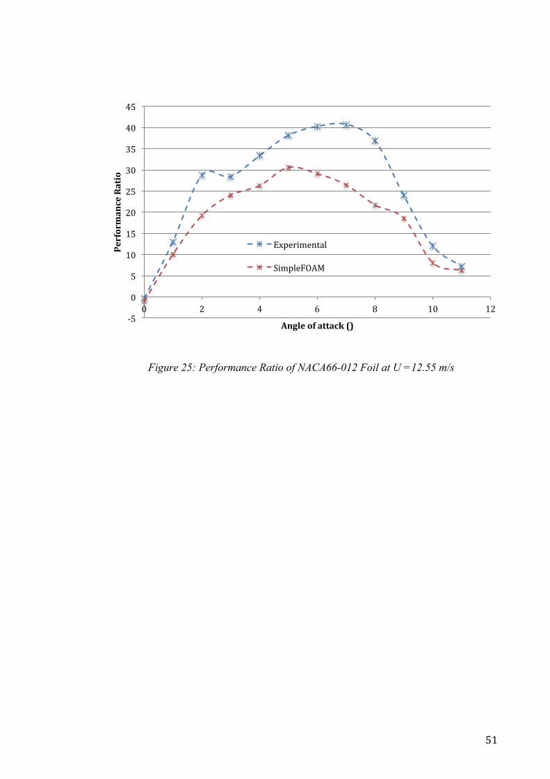
51


-‐5

0

5

10

15

20

25

30

35

40

45

0 2 4 6 8 10 12

Performance Ratio

Angle of attack ()

Experimental

SimpleFOAM

52


The final series of sub-cavitating simulations were run at a further increased flow

velocity of 17.50 m/s at positive angles of attack ranging from 0° through to 5° at 1°

increments. The reason for the further decrease in total range of angle of attack is the

same as the reason for the previous decrease, that being that for this flow velocity an

increase in angle of attack above 5 degrees will result in incipient cavitation conditions.

Following this the foil was again tested at random negative angles of attack in the same

manner as the experimental data to prove the foils symmetrical nature. From these

simulations as before coefficients for lift as well as drag and quarter chord pitching

moments were extracted. Using the same process to obtain these performance criteria,

pressure was integrated along the surface of the hydrofoil and the resulting vector split

into components and substituted into the equations defined in the background theory.

These results were then compared to experimental results from (Keerman 1956).


53



-‐0.1

0

0.1

0.2

0.3

0.4

0.5

0.6

0 1 2 3 4 5 6

CoeDicient of Lift

Angle of attack (a)

Experimental

SimpleFOAM

54



0

0.002

0.004

0.006

0.008

0.01

0.012

0.014

0.016

0 1 2 3 4 5 6

CoeDicient of Drag

Angle of attack (a)

Experimental

SimpleFOAM

-‐0.003

-‐0.002

-‐0.001

0

0.001

0.002

0.003

0.004

0.005

0 1 2 3 4 5 6

Quarter Chord pitching Mom

ent

Angle of attack (a)

Experimental

SimpleFOAM

55


-‐5

0

5

10

15

20

25

30

35

40

45

0 1 2 3 4 5 6


Angle of attack (a)

Experimental

SimpleFOAM

56


57

4.0 Simulation of NACA66-012 Foil in Cavitating Flow Conditions

Simulation of cavitating flows was achieved in much a similar manner to the sub-

cavitating cases with the exception of a number of differences. Unlike the sub-cavitating

cases where a flow velocity was set and the angle of attack changed in the case of these

simulations a flow velocity and angle of attack was set and the cavitation number was

varied by adjusting the free stream pressure of the flow. In this case the angle of attack

of the NACA66-012 foil was set at a constant 10° and the flow velocity set at 9.45

meters per second. Whilst the domain of the case was maintained, in order to accurately

model the cavitation effects the resolution of the mesh was increased with an increase in

the maximum allowable number of cells by 2 million. Additionally in the processing

phase potentialFoam was no longer used to initialize the flows as this lead to unusual

pressure distributions when running the simulation. In addition due to the incredibly

high processing power requirements for running the chosen solver model

interphaseChangeFoam turbulence modeling was removed and replaced with a laminar

scheme in order to reduce the required CPU hours for running the case. This was

implemented as to run these cases in a timely manner processing was outsourced to the

iVEC supercomputing cluster at Murdoch which had a set limit of CPU hours available.

In this simulation performance characteristics were recorded in the same manner as for

the sub-cavitating cases for fluid flows with cavitation numbers ranging from 5.4 to

0.220.

58

Figure 32: Close View Vapour Fraction at Cavitation Number k =1.518, U = 9.45 m/s

and α = 10°

Figure 33: Vapour Fraction at Cavitation Number k =0.220, U = 9.45 m/s and α = 10°

Note from the above two figures it can be seen that an increase in the cavitation number

of the system will result in a reduction of cavitation effects, generally a cavitation

number above 3 is considered a non-cavitating flow. In the conditions tested it can be

seen that for the cavitation number of k = 1.518 there is incipient level of cavitation

behind the leading edge of the hydrofoil with vapor bubbles sheading from the surface

of the hydrofoil. Note in the above figures the colors indicate the vapor fraction of the

fluid with blue indicating a complete fluid and at the opposite end of the scale indicating

complete vapor. In the case of the second figure where the cavitation number 0.220 it

59

can be seen that there is a fully developed vapor cavity formed on nearly the complete

top surface of the hydrofoil.

Figure 34: Velocity Magnitude Field at Cavitation Number k =1.518, U = 9.45 m/s and

α = 10°

Figure 35: Pressure Magnitude Field at Cavitation Number k =1.518, U = 9.45 m/s

and α = 10°

60

Figure 36: Comparison of Coefficients of Lift at U = 9.45 m/s and α = 10 °

Figure 37: Comparison of Coefficients of Drag at U = 9.45 m/s and α = 10 °

0

0.1

0.2

0.3

0.4

0.5

0.6

0.7

0.8

0.9

1

0 1 2 3 4 5 6

CoeDicient of Lift

Cavitation Number (k)

Experimental

interPhaseChangeFoam

0

0.02

0.04

0.06

0.08

0.1

0.12

0.14

0.16

0 1 2 3 4 5 6

CoeDicient of Drag


Experimental


61

Figure 38: Comparison NACA66-012 Performance Ratios at U = 9.45 m/s and α = 10 °

0

5

10

15

20

25

30

35

40

0 1 2 3 4 5 6



Experimental


62


63

5.0 Discussion

The results gained for the performance characteristics of the NACA66-012 hydrofoil in

the sub-cavitating flow as described in chapter three of this report show that the

performance predicted by the CFD techniques varied from that gained by Keerman in

1956 using experimental techniques.

For the first series of simulations using the simpleFoam model for sub-cavitating flow

at 9.45 meters per second and angles of attack ranging from 0° to 13° there is a variation

between the experimental and the CFD derived results. For the lift forces predicted at

this flow velocity the CFD results follow the trend of the experimental results of a

steady rise in force as the angle of attack is increased up to 11° where the lift forces

plateau and then start to decrease as the foil reaches the critical angle of attack (also

known as the stall angle) up to 13°. Whilst the trend is followed the actual force

predicted by the CFD technique actually exceeds the experimental data by a fairly

constant 10-15% percent. For the drag forces in this case it is a similar situation with the

CFD data following the same trend as the experimental data but again over predicting

the experienced force particularly at angles of attack of 10° or greater. The hydrofoil

performance ratio at this flow velocity shows a high correlation between the two

methods for angles 9° and greater but for angles less than this it tends to severely under

predict the performance of the hydrofoil. For the quarter chord pitching moment the

experienced forces follow a similar trend as the experimental result with a major

exception occurring at angles greater than 10 degrees where the experimental data

shows a rapid decrease to negative values whilst the CFD data shows the opposite of a

rapid increase to greater positive values.

For the second series of simulations using the simpleFoam model for sub-cavitating

flow at an increased velocity of 12.55 meters per second and a decreased series of

angles of attack ranging from 0° to 11° as with the previous result there is a variation

between the experimental and the CFD derived results. Also as with the previous data

the lift and drag forces acing on the hydrofoil at this speed follow the trend of the

64

experimental data from Keerman quite closely with a tendency to over predict the

expected forces by less than 20% in most cases. Also as with the previous case the

hydrofoil performance ratio matches quite closely with the experimental data for angles

of attack 9° or greater whilst below these angles it also tends to under predict the lift to

drag ratio of the foil.

For the third and final series of simulations using the simpleFoam model for sub-

cavitating flow at an increased velocity of 17.50 meters per second and a decreased

series of angles of attack ranging from 0° to 5° unlike the previous two sets result there

is a greater variation between the experimental and the CFD derived results. For the

coefficient of lift for this simulation the CFD results show a far reduced force for angels

of 0° and 1° then the trend crosses the experimental data and predicts lift forces far

exceeding those predicted by Keerman for greater angles. For the drag forces calculated

for these simulations the CFD data consistently predicts forces around 50% greater than

the experimental data. For the hydrofoil performance ratio at this flow velocity the CFD

data matches the experimental data quite closely for angles 2° and above however

below this particularly at 1° the CFD data shows a performance far less than the

experimental data.

The simulations of cavitating flows carried out at a constant speed of 9.45 meters per

second and constant angle of attack of +10° showed much greater variance from the

experimental data than those shown in the sub-cavitating cases. For lift forces greater

than cavitation numbers of 1.5 the force calculated using CFD techniques were quite

similar to the experimental data of Keerman however below this cavitation number the

predicted lift forces far exceeded the experimental data. For the resultant drag forces

between cavitation numbers of 0.7 and 4.5 the interPhaseChangeFoam model tended to

predict forces lower than the experimental data whilst outside these cavitation numbers

the forces tended to be greater than what would be expected. For the hydrofoil

performance ratio in this flow there is a reasonable correlation for cavitation numbers

less than 1.5 however above this point there is a rapid spike well above the experimental

data followed by a rapid decline from just above a k value of 3.

65

There are a number of possible sources of error that must be considered, which

potentially could have contributed to the variances between the experimental data and

that from the CFD simulations.

Firstly in all cases of computational fluid dynamics the design and quality of the mesh

plays an important role in the quality of the results produced. Whist it is desirable to

have as fine a mesh as possible doing so will require increasing quantities of

computational power to resolve a solution. For this reason it is important to strike a

suitable balance between quality and efficiency. Additionally some fluid dynamics

effects such as cavitation benefit from having a finer mesh specifically in the region

where such effects occur. The mesh designed for the sub-cavitating flows had a limit of

approximately 3.5 million cells with a relativity coarse domain mesh with a high level

of refinement increasing in proximity of the foil with particular interest placed on the

leading and trailing edges of the foil as these points are critical to predicting foil

performance (Ofer 2008). For the cavitating flows the mesh limit was increased by 2

million cells to 5.5 million cells with particular interest placed on the surface behind the

leading edge of the foil. Whilst these are large cell limits for such a simulation it is still

likely that there would have been some effect on the results due to this.

For the sub-cavitating flows the use of the very basic simpleFoam solver model that

does not allow for compressibility of the fluid could have contributed to the error in the

results. Whist water at the pressures experienced has less than negligible

compressibility this most basic of solvers is not an ideal solution as it does not account

for a number of hydrodynamic effects. Additionally turbulence modelling on the surface

of the hydrofoil using the RANS two-equation k-ω SST model could have also

contributed. Whist RANS turbulence modelling is one of the least processor intensive

model schemes it is known to produce poor results in comparison to a more advanced

turbulence model such as LES and is this considered to be among “the best of the

worst”.

66

In the case of the cavitating flow simulations there were also a number of possible

sources of error. Firstly cavitation is a complex phenomenon and there are large

variations in methods for modelling its effects such as models based on barotropic

equations of state or like the interPhaseChangeFoam model used based on the transport

equation of vapour fractions. The result of using different modelling methods is that

some work only in specific styles of simulations and thus the selection of the most

suitable model is important in producing accurate results. Additionally in order to save

computational power in already computationally intensive simulations turbulence was

modelled using a laminar model scheme, which could have also resulted in potential

errors in the results.

Overall the results gained for the sub-cavitating flow simulations can actually be

considered to have produced reasonable results for such a basic simulation. In the case

of the cavitating simulations whilst the data shows larger than expected discrepancy’s

between the CFD and experimental data the results of the project can again be

considered relatively good as stated by Gosset when using interPhaseChangeFoam

which is considered OpenFOAM’s best solver for hydrofoil cavitation results within an

order of magnitude are acceptable.

In hindsight there are a number of changes that could have been applied to this project

that could have resulted in procurement of better data. Whist it is acknowledged that

OpenFOAM is a particularly powerful and versatile CFD package it has a especially

steep learning curve with little documentation on the process of creating new and

customised simulations. For this reason it is considered that greater levels of co-

operation and communication between students using this package especially for the

first half of the project period would offer substantial benefits. Secondly the simulations

were set to rotate the hydrofoil at the midchord point when changing the angle of attack.

This required recalculation of the axis of rotation of the quarter chord for each

simulation. This proved to be a severe problem as the pitching moment is highly

sensitive to the positioning of this axis with the slightest variation resulting in large

discrepancy’s of the quarter chord pitching moment.

67

6.0 Conclusions

The importance of computational fluid dynamics techniques in the development of

hydrofoil design is becoming increasingly apparent as demand for larger and high

performing hydrofoil craft meets the technological wall in hydrofoil design. CFD

presents the potential for watercraft designers to increase design efficiency and reduce

development costs.




design obtained previously using experimental methods. A symmetrical NACA 66-012

section hydrofoil was selected and its performance characteristics including parameters

such as lift and drag coefficients and quarter chord pitching moments were calculated

for a range of flow velocity’s and angles of attack in sub-cavitating flow and at a

constant angle of attack with varying cavitation numbers in cavitating flows, following

this the results were compared to the known data.

Results gained from the sub-cavitating simulations shows that the forces experienced on

a hydrofoil could be predicted to within a consistent 10-15% variance from the

experimental data published by Keerman in 1956. In the case of the cavitating flow

simulations showed large variances of up to 75% between the experimental and the

CFD data. Whilst this variance would be considered large for such work according to

work published by Gosset in 2010 notes that for a simulation using the OpenFOAM

solver model selected on a symmetrical hydrofoil that results within an order of

magnitude are acceptable.

Thus the set objectives of this project were completed successfully as simulation of

flows sub-cavitating through to fully developed cavitation were modelled for the

NACA66-012 hydrofoil and the results were compared to experimental data and were

68

found to be within an acceptable level of agreement for the given software package

used.

6.1 Recommendation for Future Works.

There are a number of recommendations that could be made for future work on this

project including.

1. Increasing the range of flow velocities and angles of attack for both sub-

cavitating and especially for cavitating flow regimens.

2. Using different solvers such as rhoSimpleFoam and cavitatingFoam and

comparing the results gained both to the experimental data and those derived

during this project.

3. Add supporting structure to the foil such as what would bee seen when attaching

such a foil to a hydrofoil craft.

4. Add surface features or adjust the profile by using modifications such as fins or

bumps such as those seen on objects such as golf balls tin order to see if the

performance characteristics could be improved.

5. Simulate venting through the hydrofoil to see if the performance characteristics

could be improved.

6. Simulate interaction of the hydrofoil near a free surface to inspect the effects of

mixing on the performance of the foil.

69

7.0 References

1. R., Keerman. "Water Tunnel Tests of the Naca 66-012 Hydrofoil in Non Cavitatin

and Cavitating Flows." Pasadena California: Department of Navy, Beauro of Ships,

1956.

2. Jamieson, J.J., W.E. Farris, and BOEING CO SEATTLE WASH ADVANCED

MARINE SYSTEMS ORGANIZATION. Hydrofoil Simulation Equations Study:

Performance Criteria and Test Report for Hydrofoil Craft. Defense Technical

Information Center, 1966.

3. Versteeg H.K., Malalasekera W. An Introduction to Computational Fluid

Dynamics: The Finite Volume Method. Longman Scientific & Technical, 1995.

4. Pike, J. "Hydrofoil Limitations." (2011). Published electronically 07/07/2011.

http://www.globalsecurity.org/military/systems/ship/hydrofoil-limits.htm.

5. Gosset, A. Díaz Cásas, V. López Peña, F. "Evaluation of the Cavitatingfoam Solver

for Low Mach Number Flow around a 2d Hydrofoil." (2010).

6. Schlichting, H., and K. Gersten. Boundary-Layer Theory. MacGraw-Hill, 2000.

7. Brennen, Christopher E. "Cavitation and Bubble Dynamics." (2003).

http://caltechbook.library.caltech.edu/archive/00000001/00/chap1.htm.

8. Reynolds, Osborne. "On the Effect of Immersion on Screw Propellers."

Transactions of the Institute on Naval Architects (march 27th 1874).

9. Franc, J.P., and J.M. Michel. Fundamentals of Cavitation. Kluwer Academic

Publishers, 2006.

10. Savchenko, Yuriy N. "Supercavitation - Problems and Perspectives ", National

Academy of Sciences, 2001.

11. Thom, A. "The Flow Past Circular Cylinders at Low Speeds." Proceedings of the

Royal Society of London. Series A, Containing Papers of a Mathematical and

Physical Character 141, no. 845 (September 1st 1933): 651-69.

12. Kawaguti, Mitutosi. "Numerical Solution of the Navier-Stokes Equations for the

Flow around a Circular Cylinder at Reynolds Number 40." Journal of the Physical

Society of Japan 8, no. 6 (1953): 747-57.

70

13. Land, Norman S. "Charachteristics of a Naca 66 S-209 Hydrofoil Section Hydrofoil

at Several Depths ", edited by National advisory comittee for aeronautics. Langley

Field Va, 1943.

14. Sheng Huang, Miao He, Chao Wang, Xin Chang. "Simulation of Cavitating Flow

around a 2-D Hydrofoil." J. Marine 9 (June 6 2010): 63-16.

15. P. R. Spalart., “Strategies for turbulence modelling and simulations,” Boeing

Commercial Airlines, P.O. Box 3707, Seattle, WA 98124, USA, International

Journal of Heat and Fluid Flow, 19 February, 2000

16. Land, Norman S. "Charachteristics of a Naca 66 S-209 Hydrofoil Section Hydrofoil

at Several Depths ", edited by National advisory comittee for aeronautics. Langley

Field Va, 1943.

17. Amromin, E., Kopriva, J., Arndt, R. & Wosnik, M. (2006), Hydrofoil drag reduction

by partial cavitation, J. Fl. Eng. 128, 931-936.

18. Kjeldsen, M., Arndt, R. & Effertz, M. (2000), Spectral characteristics of sheet/cloud

cavitation, J. Fl. Eng. 122, 481-487.

19. Aharon, Ofer. "Mit - 2.094 - Term Project - Hydrofoil Analysis Using Cfd." MIT,

2008.

71

Appendices

(See Attached Disk)

CFD validation of hydrofoil performance characteristics in cavitating ...

Documents

Transcript of CFD validation of hydrofoil performance characteristics in cavitating ...