Causal effect of income on health: Investigating two closely related policy reforms in Austria

by

Mario SCHNALZENBERGER

Working Paper No. 1109 July 2011

DDEEPPAARRTTMMEENNTT OOFF EECCOONNOOMMIICCSS JJOOHHAANNNNEESS KKEEPPLLEERR UUNNIIVVEERRSSIITTYY OOFF

LLIINNZZ

Johannes Kepler University of Linz Department of Economics

Altenberger Strasse 69 A-4040 Linz - Auhof, Austria

www.econ.jku.at

mario.schnalzenberger@jku.at phone +43 (0)732 2468 -5376, -8217 (fax)

Causal effect of income on health:Investigating two closely related policy

reforms in Austria∗

Mario Schnalzenberger†

University of Linz

July, 2011

Abstract

I investigate the effect of income on mortality of the pensioners, com-paring three subsequent policy periods in Austria. The pensioners whoretired in the second period received 25% lower pension than those in thefirst period. This reduction in income was removed in the third policyperiod. These two reforms allow a causal identification of the effect of in-come on health. I estimate that lower pension did not change the mortalityrate. The results are confirmed using both experiments and different meth-ods of estimation. Furthermore, with regard to the expenditure on healthservices, I get that only prescribed drug consumption increased, with theremaining analyzed factors being unaffected.

Keywords: Income, Mortality, Health, ExpenditureJEL classification: I12, J14, H55

∗The author would like to thank the Austrian FWF for funding of the “Center for LaborEconomics and the Welfare State“. The SHARE data collection has been primarily fundedby the European Commission through the 5th, 6th and 7th framework programme, as well asfrom the U.S. National Institute on Aging and other national Funds. For helpful discussionthe author would like to give thanks to participants of the Annual Meeting of the EuropeanSociety for Population Economics 2010, the Labor Economics Seminar in Engelberg 2011, andseminars in Vienna and Linz. The usual disclaimer applies.†Address for correspondence: Johannes Kepler University of Linz, Department of Economics,

Altenbergerstr. 69, 4040 Linz, Austria, ph.: +43 70 2468 5376, fax: +43 70 2468 25376, email:mario.schnalzenberger@jku.at.

1 Introduction

Health and income are positively correlated (see, e.g., Bloom and Canning, 2000;

Rogot et al., 1992). Income might affect health and health might influence income

in many different ways. Wealthier individuals can afford more and better health

care, are able to spend more money on health prevention, can also afford to pay

more on living in better and healthier environments, and may be more sensitive

to unhealthy working conditions. “The differential use of health knowledge and

technology” (Cutler et al., 2006, p. 115) may also explain important parts of

the relation between social status (including income) and health. There are also

paths through which income may have a negative effect on health. Usually, the

effect of earning more comes with increased working hours, increased accidental

risks, and/or increased stress at work. This influence of income on health can be

described using a health production framework (Grossman, 1972).

On the other hand, health may influence labor supply, effort, and thus, income.

Smith (1998, 1999) and Wu (2003) analyze the causal effect of health on income

using unanticipated health shocks.

Scholars prefer randomized experiments to analyze the causal effect of income

on health. However, in most cases, the experiments are economically and/or

ethically not feasible1. In the cases where the effect of income on health is of

primary interest, it may seem paradoxical to pay the participants of a study to

accept less income, and it may seem offensive to take away money from randomly

drawn citizens. We rely on the exploitation of natural experiments based on the

evaluation of the policies affecting income to analyze the causal effect of income

on health.

1Thomas et al. (2006) is one of the recent exceptions.

1

The empirical literature shows a positive but not always significant causal effect

of income on health. Benzeval et al. (2000), Case (2001), and Frijters et al. (2005)

find a small causal effect of income on self-reported health. Cawley et al. (2010)

analyze the effect of reduced social security payments on the retirees’ weight and

BMI in the US and do not find any evidence for the causal effects of income on

the weight or BMI of elderly Americans. Adams et al. (2003) analyze the causal

effect of income for elderly persons in the US. They do not find any “associations

of health conditions and changes in total wealth” (p. 51) for persons aged 70

and above. Lindahl (2005) does not find any significant effect of lottery prizes on

mortality in Sweden.

In their meta study, Cutler et al. (2006) conclude with regard to the determinants

of mortality within countries that it “seems clear that much of the link between

income and health is a result of the latter causing the former, rather than the

reverse.” (p. 115) This suggests that all those findings of quantitatively small

and mostly insignificant effects are in line with their interpretation.

Switching to Austria, in May 2000, the European Court of Justice ruled that

one type of early retirement violated the European law. This decision surprised

the government and the public and the subsequent abolition of this retirement

in June 2000 can be seen as a natural experiment. Before the abolition, retirees

received up to 25 % more gross pension than thereafter. Four months after the

regime change, the replacement rate was raised to its previous high level again.

Using the data from Austrian social security records, I exploit these two changes

to study the causal effect of income on health for elderly persons.

To measure health, I use the mortality rates over a period of seven years, which

is the ultimate indicator of bad health for these elderly persons. Second, for a

2

small proportion of the individuals, the data from the public health insurance is

available. Therefore, I can use the health expenditure on drugs or medical aid,

visits to general or special practitioners, and hospital visits.

The Austrian social security records contain detailed information not only on

the employment histories but also on the health histories of all Austrian private

sector employees. I compare the cohorts aged 57 to 59 in the period January to

September 2000 for the first regime change and cohorts aged 57 to 60 in the period

June to December 2000 for the second regime change. All cohorts compared are

exposed to the same health “risks” (epidemics, etc.) all the time.

The seven year mortality values for these persons are not statistically different.

I see that only the expenditure on drugs increases significantly, but all other

expenses and measures (visits to a doctor or a hospital, expenditure on medical

aids, etc.) are unaffected.

2 Institutional Background

2.1 Austrian Pension System

Between the 1970s and the 1990s, Austria had a generous pension system that

contained various provisions for early retirement (see Hofer and Koman, 2006). In

2000, Austria spent 14.3 % of its GDP on pension expenditure (Eurostat Statistics

Database, Economic Policy Committee, 2010). Although the regular retirement

age is similar to that in other European countries (65 for men and 60 for women),

the actual retirement age of men decreased steadily from nearly 62 in the 1970s

to about 58 in 1995. Since then, it has increased slightly to 58.5 in 2000 and has

stayed around 59 since 2005 (Hauptverband der osterr. Sozialversicherungstrager,

3

2010). The large share of pension expenditure in the GDP and the low retirement

age is accompanied by one of the lowest participation rates of elderly men and

women amongst the OECD countries (Organisation for Economic Co-operation

and Development, 2006).

Up to the year 2000, several early retirement schemes enabled men aged 60 and

women aged 55 to retire early, e.g., for those who have been insured for long or

are unemployed. Early retirement due to reduced working capacity was possible

for men aged 57 and above. For males, the only other alternative to retire at

the age of 59 or earlier was the invalidity pension (IP). For both alternatives, a

doctor has to check whether or not the applicant had reduced working capacity.2

The calculation of pension benefits is based on the number of years insured (the

contribution years) as a basis for the replacement rate. The pension amount

is calculated on the basis of the average monthly earnings in the best 15 years

of contribution with an average net replacement ratio of 75% (Organisation for

Economic Co-operation and Development, 2005).3

2.2 Invalidity Pension versus Early Retirement due to Re-

duced Working Capacity

In 1993, the Austrian government introduced multiple new provisions for early

retirement. One of these was the “Early Retirement due to Reduced Working

Capacity” (ERRWC). This provision was introduced for older workers with re-

duced working capacity as another form of retirement (along with the invalidity

pension). The main difference between the two schemes is a higher replacement

2I concentrate on men because the reforms were not effective for women.3A detailed description of the calculation of pension benefits in the Austrian pension system

can be found in Manoli et al. (2009).

4

rate for the workers retiring under the ERRWC (details later). The introduction

was announced months before, and hence, individuals could have adapted easily

by postponing their retirement decision. Thus, the introduction of the ERRWC

does not qualify for a natural experiment.

In May 2000, the European Court of Justice ruled that the ERRWC violated

European Law, because the difference in the retirement age for men and women

discriminated against men. The decision blindsided the government and the

public in Austria. The ERRWC was abolished immediately. Before the abolition,

retirees received a higher pension. After the abolition employees with reduced

working capacity could only apply for the IP. Using this natural experiment, I

can study the effect of income on health.

Under all regimes and for both types, the ERRWC and the IP, an individual, who

wanted to retire, had to be declared as being disabled using the same medical

checkup at the Austrian pension insurance agency. The same physicians evaluated

these pension applicants in the same rooms, using exactly the same procedures

and medical tests. The applicants were randomly assigned to the physicians.4

While both types focused on reduced working capacity, the ERRWC additionally

required a larger job history for eligibility (working six years in the last 15 years).

For the empirical comparisons between ERRWC and IP below, I only consider

the individuals fulfilling this criterion of eligibility.

The exact differences in the replacement rates (i.e., in the resulting pension ben-

efits) of the two regimes can be seen in Figure 1a. The graph shows the exact

replacement rate for a male employee aged 57 to 59 with a varying number of

contribution years on the x-axis. If this employee contributed for up to 36 years

to the public pension insurance, he would have received the same pension benefits

4This has also been confirmed by the Austrian public pension insurance agency.

5

in both regimes. Any further increase in the number of contribution years widens

the gap in the replacement rate.

Immediately after the abolition of the ERRWC, the government discussed the

situation of pension applicants with reduced working capacity and consequently,

removed the replacement rate cap of 60% on the IP and slightly revised the

calculation of the replacement rate. The resulting replacement rate differences

between the two IP regimes can be found in Figure 1b. As compared to the

previous case, both regimes are identical except for the replacement rate; there

is no need to control for the number of years insured in the last 15 years.

Due to the presence of a different pension regime before 2000, I only consider the

employees who retired in 2000. Until June 2000, the ERRWC regime with a high

replacement rate was in place (regime 1). The applicants to the ERRWC in May

(at the time of its abolition) started receiving pension benefits in June. Following

this, only the IP regime with the replacement rate cap remained until the end

of September 2000 (regime 2). These retirees received reduced pension benefits

for at least seven years. From October 2000 onwards, the IP was changed with

respect to its replacement rate cap (regime 3).

6

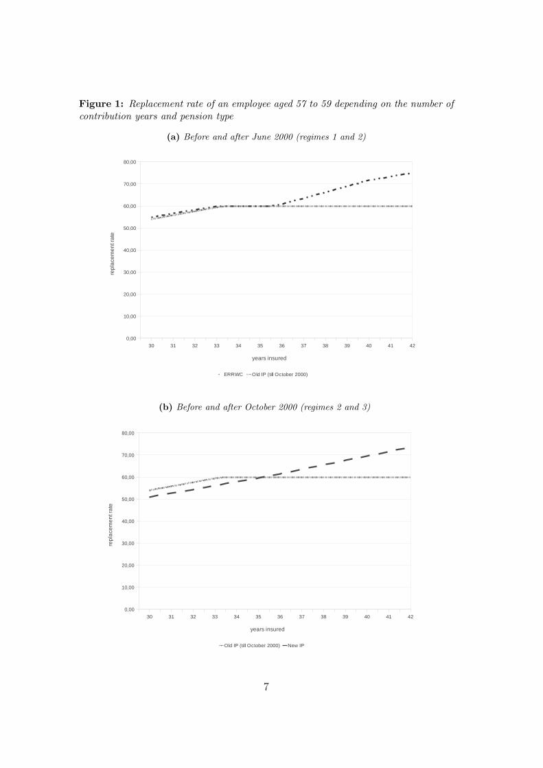
Figure 1: Replacement rate of an employee aged 57 to 59 depending on the number ofcontribution years and pension type

(a) Before and after June 2000 (regimes 1 and 2)

Calculus based on insurance years

Seite 1

30 31 32 33 34 35 36 37 38 39 40 41 42

0,00

10,00

20,00

30,00

40,00

50,00

60,00

70,00

80,00

ERRWC Old IP (till October 2000)

years insured

rep

lace

me

nt r

ate

(b) Before and after October 2000 (regimes 2 and 3)

Calculus based on insurance years

Seite 1

30 31 32 33 34 35 36 37 38 39 40 41 42

0,00

10,00

20,00

30,00

40,00

50,00

60,00

70,00

80,00

Old IP (till October 2000) New IP

years insured

rep

lace

me

nt r

ate

7

3 Data

I use the administrative employment records from the Austrian social security

system covering the years 1972 to 2009 in detail (Zweimuller et al., 2009). The

records include very detailed data on employers, employees, and employment

spells for all private sector employees. Some information on the type of employ-

ment was recorded retrospectively even up to 1955 and before. This data set also

includes the exact date of death that forms the base for my first objective health

measure: mortality.

In addition, I use the public health insurance records of Upper Austria (a state

in Austria, with about one tenth of the country’s population). Again, only the

private sector employees are included. The public health insurance office collects

all information about the patient-specific health expenditure, most of which is

stored on a quarterly basis. Some of the expenses can be associated with special

drugs or diagnoses.

Figure 2a shows the inflow of IP and ERRWC retirees in the years 1999 to 2001.

The IP retirees were only taken into account if they fulfilled the stronger require-

ment of the ERRWC5, and as such, not all invalidity retirees are included. In

June 2000, there was a significant reduction in the inflow of retirees with reduced

working capacity because of the abolition of the ERRWC.6

5An ERRWC retiree should have worked six years in the last 15 years.6Figures 2a and 2b show the presence of ERRWC retirees even after June 2000. Some

retirees had to postpone their retirement due to additional payments at the end of their (long)employment. A minority had sued the pension agency on being eligible to that pension andwere, therefore, recorded later on.

8

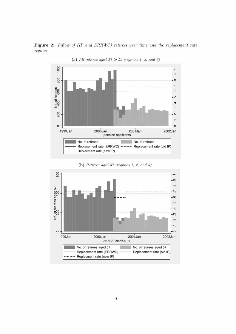
Figure 2: Inflow of (IP and ERRWC) retirees over time and the replacement rateregime

(a) All retirees aged 57 to 59 (regimes 1, 2, and 3)

0.1

.2.3

.4.5

.6.7

.8.9

1

02

00

40

06

00

80

01

00

0N

o.

of

retire

es

1999Jan 2000Jan 2001Jan 2002Janpension applicants

No. of retirees No. of retirees

Replacement rate (ERRWC) Replacement rate (old IP)

Replacment rate (new IP)

(b) Retirees aged 57 (regimes 1, 2, and 3)

0.1

.2.3

.4.5

.6.7

.8.9

1

02

00

40

06

00

No

. o

f re

tire

es a

ge

d 5

7

1999Jan 2000Jan 2001Jan 2002Janpension applicants

No. of retirees aged 57 No. of retirees aged 57

Replacement rate (ERRWC) Replacement rate (old IP)

Replacment rate (new IP)

9

Due to the changes in the general inflow of retirees, one could presume that the

older retirees could have been different. As such, I restrict the sample to those

individuals who were exactly 57 years old in all regimes (Figure 2b). There is no

significant change either because the regime with lower retirement income lasted

only for four months or because the inflow of retirees did not differ between

younger and older retirees.

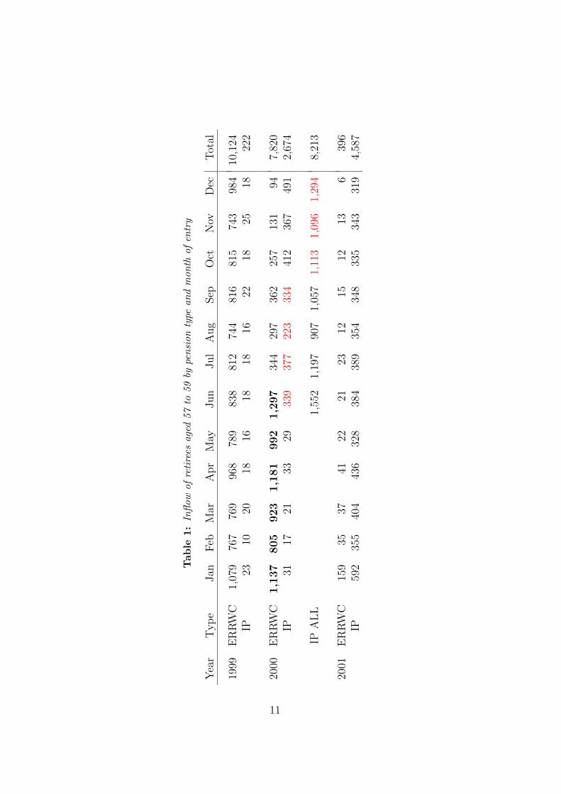
Table 1 shows all male retirees by month of entry and pension type. I study the

effect of the abolition of the ERRWC in the end of May 2000 by constructing a first

sample. This sample contains the ERRWC retirees from January to June 2000

(regime 1) and the IP retirees from June to September 2000 (regime 2). These

correspond to the rows labeled “ERRWC” and “IP” in Table 1, respectively.

The removal of the replacement rate cap four months later will be analyzed using

all IP retirees (i.e., with no restriction on the contribution years) from July to

December 2000 (regimes 2 and 3); this corresponds to the row“IP ALL”in Table 1.

Here, the retirees from October onwards (regime 3) receive a higher replacement

rate for the same number of contribution years.

Health can be measured in various ways. Many authors use self-reported health

indicators (Contoyannis et al., 2004; Frijters et al., 2005), while others measure

health on the basis of objective variables such as BMI, weight (Cawley et al.,

2010) – and mortality (see especially Cutler et al., 2006). In this paper, I use the

7-year mortality risk as the main health outcome. In 2000, the 7-year mortality

risk was 8.3% for 57 years old men and 9.9% for 59 years old men (see Statistik

Austria (2011), mortality table 2000). In the samples, the mean mortality was

7.5% for the ERRWC retirees and 8% for the IP retirees, which is slightly lower

than the mortality risk for the whole male population aged 57 to 59.

10

Table

1:

Infl

ow

of

reti

rees

age

d57

to59

bype

nsi

on

type

an

dm

on

thof

entr

y

Yea

rT

yp

eJan

Feb

Mar

Apr

May

Jun

Jul

Aug

Sep

Oct

Nov

Dec

Tot

al

1999

ER

RW

C1,

079

767

769

968

789

838

812

744

816

815

743

984

10,1

24IP

2310

2018

1618

1816

2218

2518

222

2000

ER

RW

C1,1

37

805

923

1,1

81

992

1,2

97

344

297

362

257

131

947,

820

IP31

1721

3329

339

377

223

334

412

367

491

2,67

4

IPA

LL

1,55

21,

197

907

1,05

71,

113

1,09

61,

294

8,21

3

2001

ER

RW

C15

935

3741

2221

2312

1512

136

396

IP59

235

540

443

632

838

438

935

434

833

534

331

94,

587

11

Measuring health by mortality is a rather conservative approach because mortal-

ity will react only if health is strongly affected by the treatment. Therefore, I

construct a second set of health measures through which the treatment may affect

health. Using the data of the public health insurance records of Upper Austria,

I calculate variables such as the number of visits to a general practitioner or

specialist, health expenditure on prescribed medical drugs or medical aids, and

the number of days in a hospital. These variables may be more sensitive to the

treatments but may also bear more variation due to other factors that might be

correlated with the treatment.

4 Empirical Strategy

4.1 Abolition of the ERRWC

The pension regulations themselves match only the people with the minimum

level of reduced working capacity in all three regimes. Nevertheless, this proce-

dure establishes only some degree of randomization. After May 2000, the first

reform, the individuals are still able to self-select into treatment by choosing not

to retire at all.

Table 8 in the Appendix shows the descriptive statistics of the two groups before

and after the first reform (column “First Sample”). The differences in the recent

and 15-year employment history are not significant but seem to be relevant. The

IP pensioners are slightly less healthy, more often unemployed, and therefore, less

often at work. Looking at the individual characteristics, education is different for

the two groups, and so is citizenship to a small extent.

12

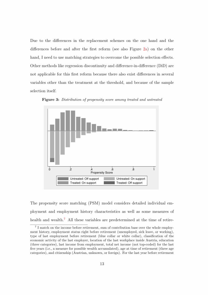
Due to the differences in the replacement schemes on the one hand and the

differences before and after the first reform (see also Figure 2a) on the other

hand, I need to use matching strategies to overcome the possible selection effects.

Other methods like regression discontinuity and difference-in-difference (DiD) are

not applicable for this first reform because there also exist differences in several

variables other than the treatment at the threshold, and because of the sample

selection itself.

Figure 3: Distribution of propensity score among treated and untreated

0 .2 .4 .6 .8 1Propensity Score

Untreated: Off support Untreated: On support

Treated: On support Treated: Off support

The propensity score matching (PSM) model considers detailed individual em-

ployment and employment history characteristics as well as some measures of

health and wealth.7 All these variables are predetermined at the time of retire-

7 I match on the income before retirement, sum of contribution base over the whole employ-ment history, employment status right before retirement (unemployed, sick leave, or working),type of last employment before retirement (blue collar or white collar), classification of theeconomic activity of the last employer, location of the last workplace inside Austria, education(three categories), last income from employment, total net income (not top-coded) for the lastfive years (i.e., a measure for possible wealth accumulated), age at time of retirement (three agecategories), and citizenship (Austrian, unknown, or foreign). For the last year before retirement

13

ment. Using a logit estimation for the propensity score, the balancing property is

fulfilled, with the region of common support being in the interval [0.007, 0.968] and

substantially large (see also Figure 3). Only 0.6 percent of the treated and about

3 percent of the controls are off support. Finally, I use various matching meth-

ods (nearest neighbor, local linear regression matching, stratification matching,

kernel matching, and a control function approach) to evaluate the causal effect

of the reform on the 7-year mortality rate of the sampled retirees.

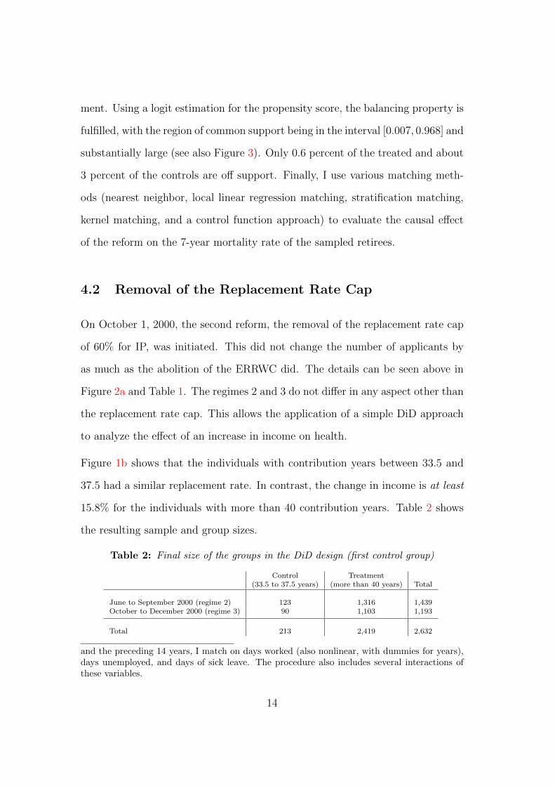
4.2 Removal of the Replacement Rate Cap

On October 1, 2000, the second reform, the removal of the replacement rate cap

of 60% for IP, was initiated. This did not change the number of applicants by

as much as the abolition of the ERRWC did. The details can be seen above in

Figure 2a and Table 1. The regimes 2 and 3 do not differ in any aspect other than

the replacement rate cap. This allows the application of a simple DiD approach

to analyze the effect of an increase in income on health.

Figure 1b shows that the individuals with contribution years between 33.5 and

37.5 had a similar replacement rate. In contrast, the change in income is at least

15.8% for the individuals with more than 40 contribution years. Table 2 shows

the resulting sample and group sizes.

Table 2: Final size of the groups in the DiD design (first control group)

Control Treatment(33.5 to 37.5 years) (more than 40 years) Total

June to September 2000 (regime 2) 123 1,316 1,439October to December 2000 (regime 3) 90 1,103 1,193

Total 213 2,419 2,632

and the preceding 14 years, I match on days worked (also nonlinear, with dummies for years),days unemployed, and days of sick leave. The procedure also includes several interactions ofthese variables.

14

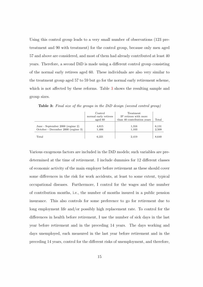
Using this control group leads to a very small number of observations (123 pre-

treatment and 90 with treatment) for the control group, because only men aged

57 and above are considered, and most of them had already contributed at least 40

years. Therefore, a second DiD is made using a different control group consisting

of the normal early retirees aged 60. These individuals are also very similar to

the treatment group aged 57 to 59 but go for the normal early retirement scheme,

which is not affected by these reforms. Table 3 shows the resulting sample and

group sizes.

Table 3: Final size of the groups in the DiD design (second control group)

Control Treatmentnormal early retirees IP retirees with more

aged 60 than 40 contribution years Total

June - September 2000 (regime 2) 4,815 1,316 6,131October - December 2000 (regime 3) 1,406 1,103 2,509

Total 6,221 2,419 8,640

Various exogenous factors are included in the DiD models; such variables are pre-

determined at the time of retirement. I include dummies for 12 different classes

of economic activity of the main employer before retirement as these should cover

some differences in the risk for work accidents, at least to some extent, typical

occupational diseases. Furthermore, I control for the wages and the number

of contribution months, i.e., the number of months insured in a public pension

insurance. This also controls for some preference to go for retirement due to

long employment life and/or possibly high replacement rate. To control for the

differences in health before retirement, I use the number of sick days in the last

year before retirement and in the preceding 14 years. The days working and

days unemployed, each measured in the last year before retirement and in the

preceding 14 years, control for the different risks of unemployment, and therefore,

15

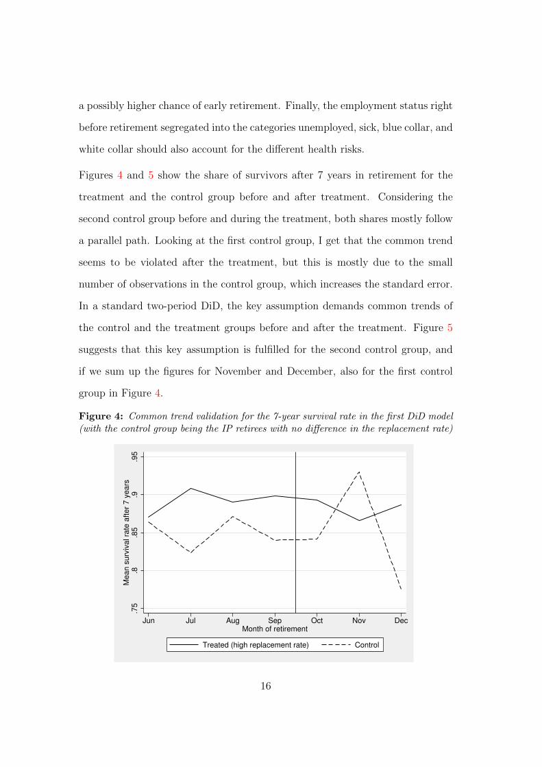
a possibly higher chance of early retirement. Finally, the employment status right

before retirement segregated into the categories unemployed, sick, blue collar, and

white collar should also account for the different health risks.

Figures 4 and 5 show the share of survivors after 7 years in retirement for the

treatment and the control group before and after treatment. Considering the

second control group before and during the treatment, both shares mostly follow

a parallel path. Looking at the first control group, I get that the common trend

seems to be violated after the treatment, but this is mostly due to the small

number of observations in the control group, which increases the standard error.

In a standard two-period DiD, the key assumption demands common trends of

the control and the treatment groups before and after the treatment. Figure 5

suggests that this key assumption is fulfilled for the second control group, and

if we sum up the figures for November and December, also for the first control

group in Figure 4.

Figure 4: Common trend validation for the 7-year survival rate in the first DiD model(with the control group being the IP retirees with no difference in the replacement rate)

.75

.8.8

5.9

.95

Me

an

su

rviv

al ra

te a

fte

r 7

ye

ars

Jun Jul Aug Sep Oct Nov DecMonth of retirement

Treated (high replacement rate) Control

16

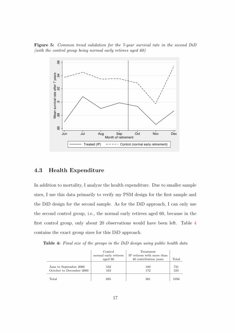
Figure 5: Common trend validation for the 7-year survival rate in the second DiD(with the control group being normal early retirees aged 60)

.86

.88

.9.9

2.9

4.9

6M

ea

n s

urv

iva

l ra

te a

fte

r 7

ye

ars

Jun Jul Aug Sep Oct Nov DecMonth of retirement

Treated (IP) Control (normal early retirement)

4.3 Health Expenditure

In addition to mortality, I analyze the health expenditure. Due to smaller sample

sizes, I use this data primarily to verify my PSM design for the first sample and

the DiD design for the second sample. As for the DiD approach, I can only use

the second control group, i.e., the normal early retirees aged 60, because in the

first control group, only about 20 observations would have been left. Table 4

contains the exact group sizes for this DiD approach.

Table 4: Final size of the groups in the DiD design using public health data

Control Treatmentnormal early retirees IP retirees with more than

aged 60 40 contribution years Total

June to September 2000 532 189 721October to December 2000 163 172 335

Total 695 361 1056

17

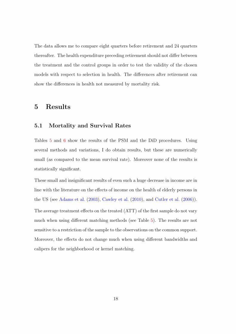
The data allows me to compare eight quarters before retirement and 24 quarters

thereafter. The health expenditure preceding retirement should not differ between

the treatment and the control groups in order to test the validity of the chosen

models with respect to selection in health. The differences after retirement can

show the differences in health not measured by mortality risk.

5 Results

5.1 Mortality and Survival Rates

Tables 5 and 6 show the results of the PSM and the DiD procedures. Using

several methods and variations, I do obtain results, but these are numerically

small (as compared to the mean survival rate). Moreover none of the results is

statistically significant.

These small and insignificant results of even such a huge decrease in income are in

line with the literature on the effects of income on the health of elderly persons in

the US (see Adams et al. (2003), Cawley et al. (2010), and Cutler et al. (2006)).

The average treatment effects on the treated (ATT) of the first sample do not vary

much when using different matching methods (see Table 5). The results are not

sensitive to a restriction of the sample to the observations on the common support.

Moreover, the effects do not change much when using different bandwidths and

calipers for the neighborhood or kernel matching.

18

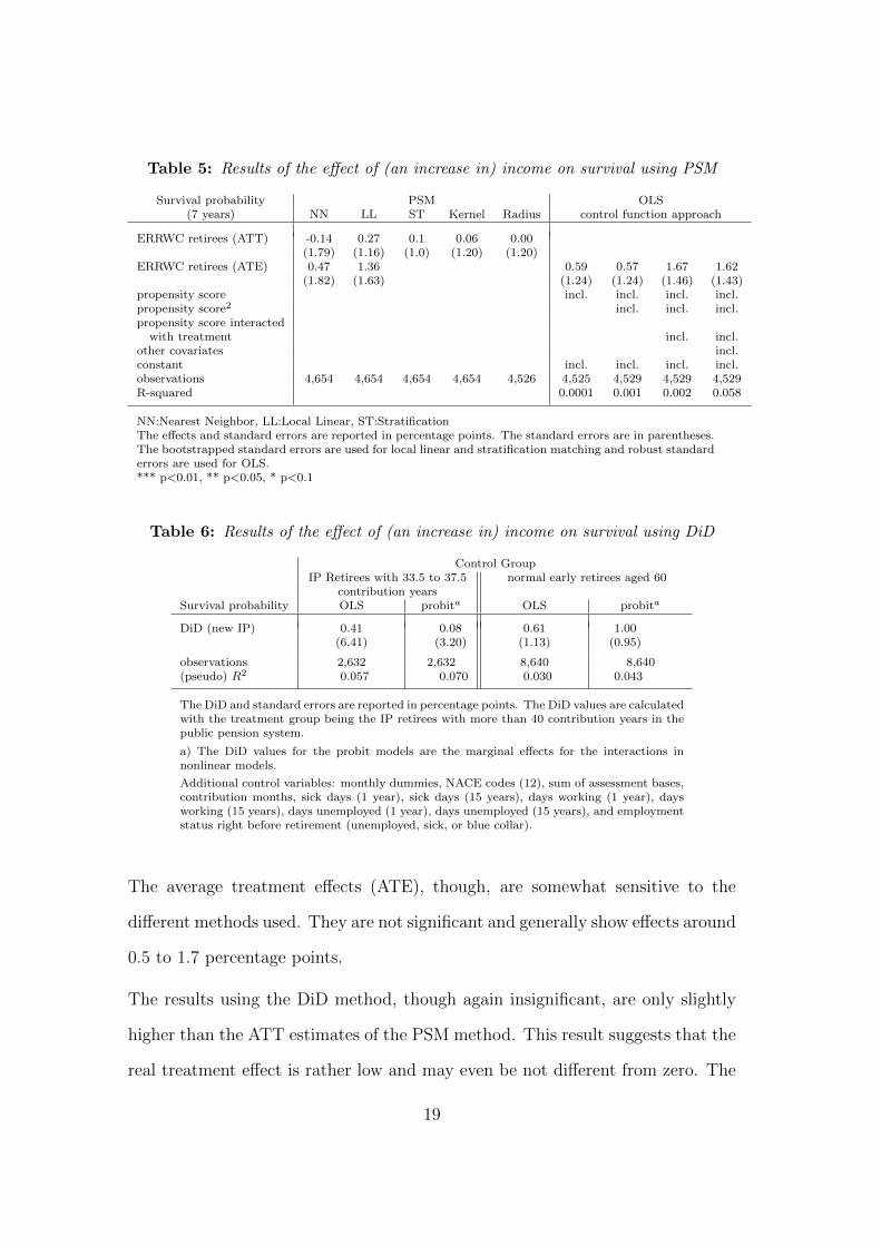
Table 5: Results of the effect of (an increase in) income on survival using PSM

Survival probability PSM OLS(7 years) NN LL ST Kernel Radius control function approach

ERRWC retirees (ATT) -0.14 0.27 0.1 0.06 0.00(1.79) (1.16) (1.0) (1.20) (1.20)

ERRWC retirees (ATE) 0.47 1.36 0.59 0.57 1.67 1.62(1.82) (1.63) (1.24) (1.24) (1.46) (1.43)

propensity score incl. incl. incl. incl.propensity score2 incl. incl. incl.propensity score interacted

with treatment incl. incl.other covariates incl.constant incl. incl. incl. incl.observations 4,654 4,654 4,654 4,654 4,526 4,525 4,529 4,529 4,529R-squared 0.0001 0.001 0.002 0.058

NN:Nearest Neighbor, LL:Local Linear, ST:StratificationThe effects and standard errors are reported in percentage points. The standard errors are in parentheses.The bootstrapped standard errors are used for local linear and stratification matching and robust standarderrors are used for OLS.*** p<0.01, ** p<0.05, * p<0.1

Table 6: Results of the effect of (an increase in) income on survival using DiD

Control GroupIP Retirees with 33.5 to 37.5 normal early retirees aged 60

contribution yearsSurvival probability OLS probita OLS probita

DiD (new IP) 0.41 0.08 0.61 1.00(6.41) (3.20) (1.13) (0.95)

observations 2,632 2,632 8,640 8,640(pseudo) R2 0.057 0.070 0.030 0.043

The DiD and standard errors are reported in percentage points. The DiD values are calculatedwith the treatment group being the IP retirees with more than 40 contribution years in thepublic pension system.

a) The DiD values for the probit models are the marginal effects for the interactions innonlinear models.

Additional control variables: monthly dummies, NACE codes (12), sum of assessment bases,contribution months, sick days (1 year), sick days (15 years), days working (1 year), daysworking (15 years), days unemployed (1 year), days unemployed (15 years), and employmentstatus right before retirement (unemployed, sick, or blue collar).

The average treatment effects (ATE), though, are somewhat sensitive to the

different methods used. They are not significant and generally show effects around

0.5 to 1.7 percentage points.

The results using the DiD method, though again insignificant, are only slightly

higher than the ATT estimates of the PSM method. This result suggests that the

real treatment effect is rather low and may even be not different from zero. The

19

DiD estimates are not sensitive to the inclusion of interactions and quadratics in

sickness information nor to the inclusion of monthly dummies (i.e., a nonlinear

time trend). Neither the point estimate nor the standard errors are affected.

5.2 Health Expenditure

With regard to the health expenditure, my samples cover quite few individuals.

First, I use the data on the health expenditure eight months preceding retirement

to verify the model with respect to the selection into treatment. Second, the effect

of the increase in income on those outcomes is analyzed. I use the expenditure on

drugs, expenditure on and number of medical aids, number of visits to a general

practitioner (GP), number of visits to a specialist, and the number of days spent

in a hospital.

The patients have to pay deductibles on drugs, medical aids, and days spent in

a hospital, while for the rest, all expenses are covered by the insurance. The

deductibles on drugs are rather low as compared to those on medical aids and

days spent in a hospital (per day fee). As for the days spent in a hospital, a

patient can leave a hospital earlier if he or she wants to, and some of the patients

may have done this to save money, which might lead to a negative effect on this

outcome due to the reduction in income.

Figures 6 and 7 show the effects of the decrease in income on the health ex-

penditure outcomes. The graphs show the difference in the health expenditure

outcomes (using the PSM or the DiD model) on the y-axis and the quarter before

and after retirement on the x-axis. Using the quarterly results, I get that there

are no significant differences before treatment, suggesting that the selection into

treatment by health status can be ruled out using this data.

20

The graphs suggest some positive (but insignificant) increase in the drugs pre-

scribed and in the number of visits to a specialist on the one hand, and a very

slight decrease (again insignificant) in the number of days spent in a hospital

after retirement.

Finally, Table 7 shows the results of the PSM (using local linear regression match-

ing) and DiD models for the aggregated pre and post retirement outcomes. All

the pre-retirement outcomes are not significant, which again suggests that the

selection into treatment by health status can be ruled out.

In the DiD model, I find a significant increase in the expenditure on medicines/drugs

for the retirees under a lower replacement rate. This may be due to the relatively

lower health due to the lower income. The medication may prevent the ultimate

health outcome, mortality, from having an effect on the treatment.

Moreover, the following effects are worth mentioning: the number of medical

aids and the number of hospital days decreased after retiring under a lower re-

placement rate. Though, these effects are not significant, they can be considered

reasonable as the patient would have to cover the relatively higher deductibles

for such services. Since the retirees already have to bear their lower pension, they

will try to avoid additional expenses such as deductibles.

21

Figure 6: PSM (local linear regression) differences in the effect of decrease in incomeon the health expenditure after the first regime change (regimes 1 and 2)

(a) Amount spent on medicines prescribed

−50

050

100

150

Am

ount spent

−10 0 10 20 30quarter

DD 95% CI upper bound

95% CI lower bound

(b) Number of visits to a GP

−4

−2

02

46

Num

ber

of vis

its

−10 0 10 20 30quarter

DD 95% CI upper bound

95% CI lower bound

(c) Amount spent on medical aids

−50

050

100

150

200

Am

ount spent

−10 0 10 20 30quarter

DD 95% CI upper bound

95% CI lower bound

(d) Number of visits to a specialist−

10

12

3N

um

ber

of vis

its

−10 0 10 20 30quarter

DD 95% CI upper bound

95% CI lower bound

(e) Number of medical aids

−20

020

40

60

Num

ber

of m

edic

al aid

s

−10 0 10 20 30quarter

DD 95% CI upper bound

95% CI lower bound

(f) Number of days spent in a hospital

−2

02

46

Num

ber

of days

−10 0 10 20 30quarter

DD 95% CI upper bound

95% CI lower bound

22

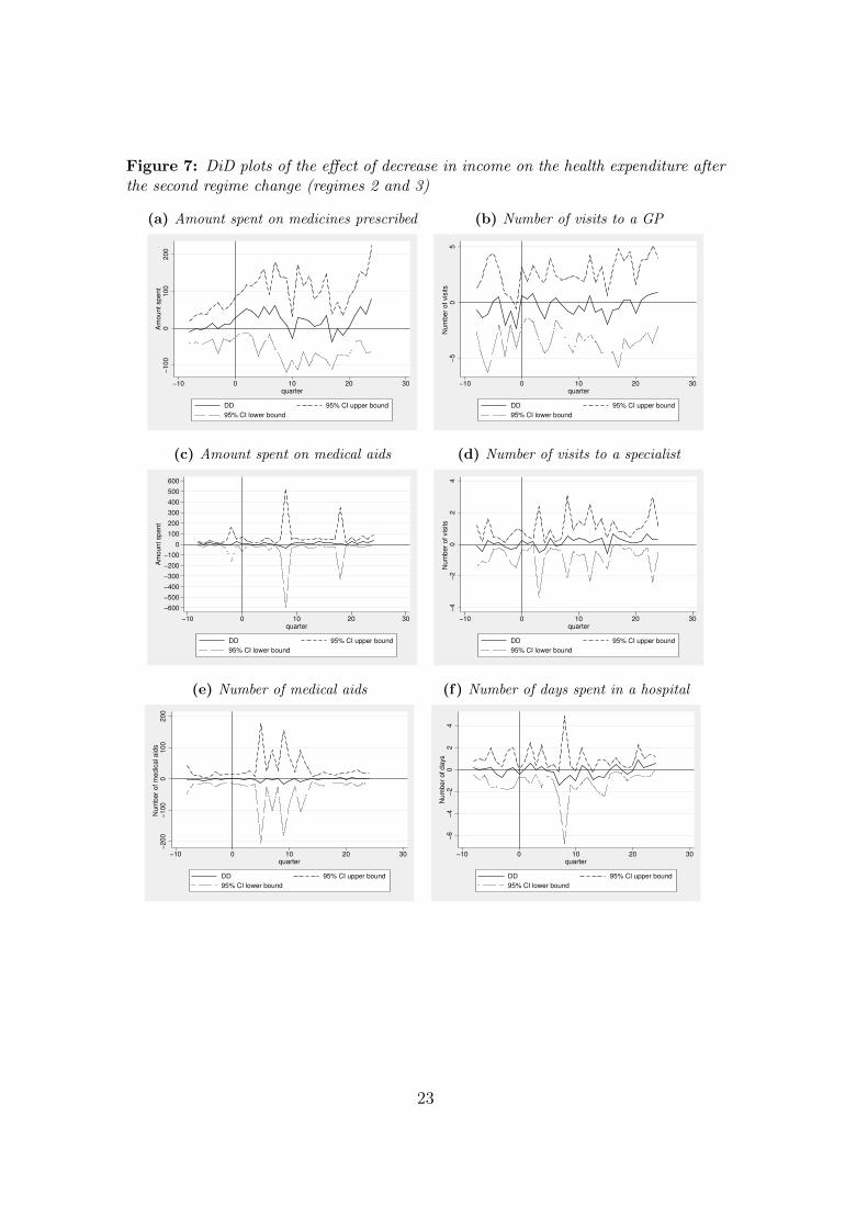
Figure 7: DiD plots of the effect of decrease in income on the health expenditure afterthe second regime change (regimes 2 and 3)

(a) Amount spent on medicines prescribed

−100

0100

200

Am

ount spent

−10 0 10 20 30quarter

DD 95% CI upper bound

95% CI lower bound

(b) Number of visits to a GP

−5

05

Num

ber

of vis

its

−10 0 10 20 30quarter

DD 95% CI upper bound

95% CI lower bound

(c) Amount spent on medical aids

−600

−500

−400

−300

−200

−100

0

100

200

300

400

500

600

Am

ount spent

−10 0 10 20 30quarter

DD 95% CI upper bound

95% CI lower bound

(d) Number of visits to a specialist−

4−

20

24

Num

ber

of vis

its

−10 0 10 20 30quarter

DD 95% CI upper bound

95% CI lower bound

(e) Number of medical aids

−200

−100

0100

200

Num

ber

of m

edic

al aid

s

−10 0 10 20 30quarter

DD 95% CI upper bound

95% CI lower bound

(f) Number of days spent in a hospital

−6

−4

−2

02

4N

um

ber

of days

−10 0 10 20 30quarter

DD 95% CI upper bound

95% CI lower bound

23

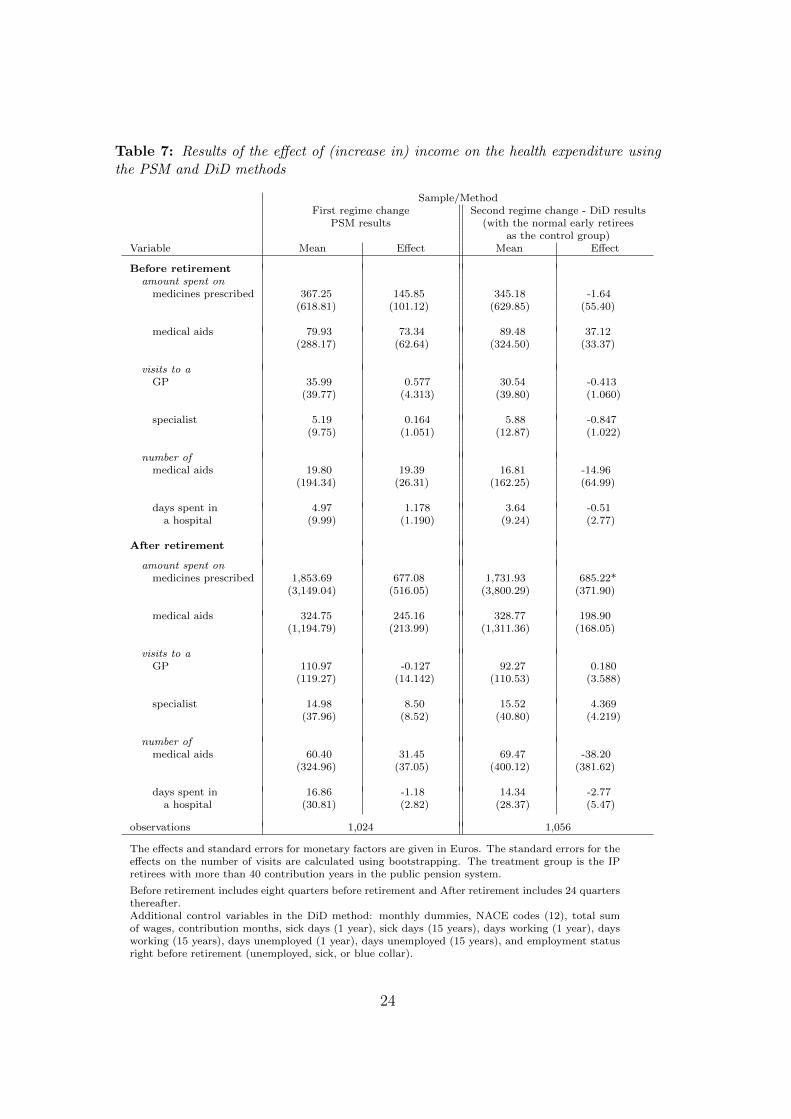
Table 7: Results of the effect of (increase in) income on the health expenditure usingthe PSM and DiD methods

Sample/MethodFirst regime change Second regime change - DiD results

PSM results (with the normal early retireesas the control group)

Variable Mean Effect Mean Effect

Before retirementamount spent on

medicines prescribed 367.25 145.85 345.18 -1.64(618.81) (101.12) (629.85) (55.40)

medical aids 79.93 73.34 89.48 37.12(288.17) (62.64) (324.50) (33.37)

visits to aGP 35.99 0.577 30.54 -0.413

(39.77) (4.313) (39.80) (1.060)

specialist 5.19 0.164 5.88 -0.847(9.75) (1.051) (12.87) (1.022)

number ofmedical aids 19.80 19.39 16.81 -14.96

(194.34) (26.31) (162.25) (64.99)

days spent in 4.97 1.178 3.64 -0.51a hospital (9.99) (1.190) (9.24) (2.77)

After retirement

amount spent onmedicines prescribed 1,853.69 677.08 1,731.93 685.22*

(3,149.04) (516.05) (3,800.29) (371.90)

medical aids 324.75 245.16 328.77 198.90(1,194.79) (213.99) (1,311.36) (168.05)

visits to aGP 110.97 -0.127 92.27 0.180

(119.27) (14.142) (110.53) (3.588)

specialist 14.98 8.50 15.52 4.369(37.96) (8.52) (40.80) (4.219)

number ofmedical aids 60.40 31.45 69.47 -38.20

(324.96) (37.05) (400.12) (381.62)

days spent in 16.86 -1.18 14.34 -2.77a hospital (30.81) (2.82) (28.37) (5.47)

observations 1,024 1,056

The effects and standard errors for monetary factors are given in Euros. The standard errors for theeffects on the number of visits are calculated using bootstrapping. The treatment group is the IPretirees with more than 40 contribution years in the public pension system.

Before retirement includes eight quarters before retirement and After retirement includes 24 quartersthereafter.Additional control variables in the DiD method: monthly dummies, NACE codes (12), total sumof wages, contribution months, sick days (1 year), sick days (15 years), days working (1 year), daysworking (15 years), days unemployed (1 year), days unemployed (15 years), and employment statusright before retirement (unemployed, sick, or blue collar).

24

6 Conclusion

The analysis shows that income has no causal effect on the mortality rates of

old aged persons in Austria. Two different natural experiments of closely related

policy reforms are analyzed using a PSM with various matching methods and a

DiD model. The distance between the two cohorts being compared by the chosen

methods is at most eight months. This implies that two close (if not the “same”)

cohorts are compared during the same period of time. These cohorts are exposed

to the same risks such as epidemics or pandemics. My results are in line with the

results of the literature on the effects of income on health for old aged individuals

in the US (Adams et al., 2003; Cawley et al., 2010; Cutler et al., 2006).

Usually, the effect of earning more is no free lunch: it comes along with increased

stress and/or increased working hours. This effect is ruled out by focusing only

on pensioners. Using the detailed data from the Austrian social security records,

both evaluations result in a low and insignificant effect on mortality compared

to the large reduction in income. One reason for this result may be the very

generous Austrian public health insurance system.

Focusing on other health-related outcomes, I can only access the data of one

state, which covers fewer individuals. First, I use the data to verify the model

with respect to the selection effects for the different types of pensions. The results

for public health expenses and the number of visits to a doctor or a hospital before

the retirement suggest that the identification strategy works and that the selection

effects can be ruled out.

Second, the effect of decrease in income on other health-related outcomes after

retirement is analyzed. Only the expenses on prescribed drugs increased signifi-

cantly at a 10 percent level due to the loss in income. For the other health-related

25

outcomes, such as the number of visits to a general practitioner, a specialist, and

a hospital, and the expenditure on medical aids, no significant effects were found.

26

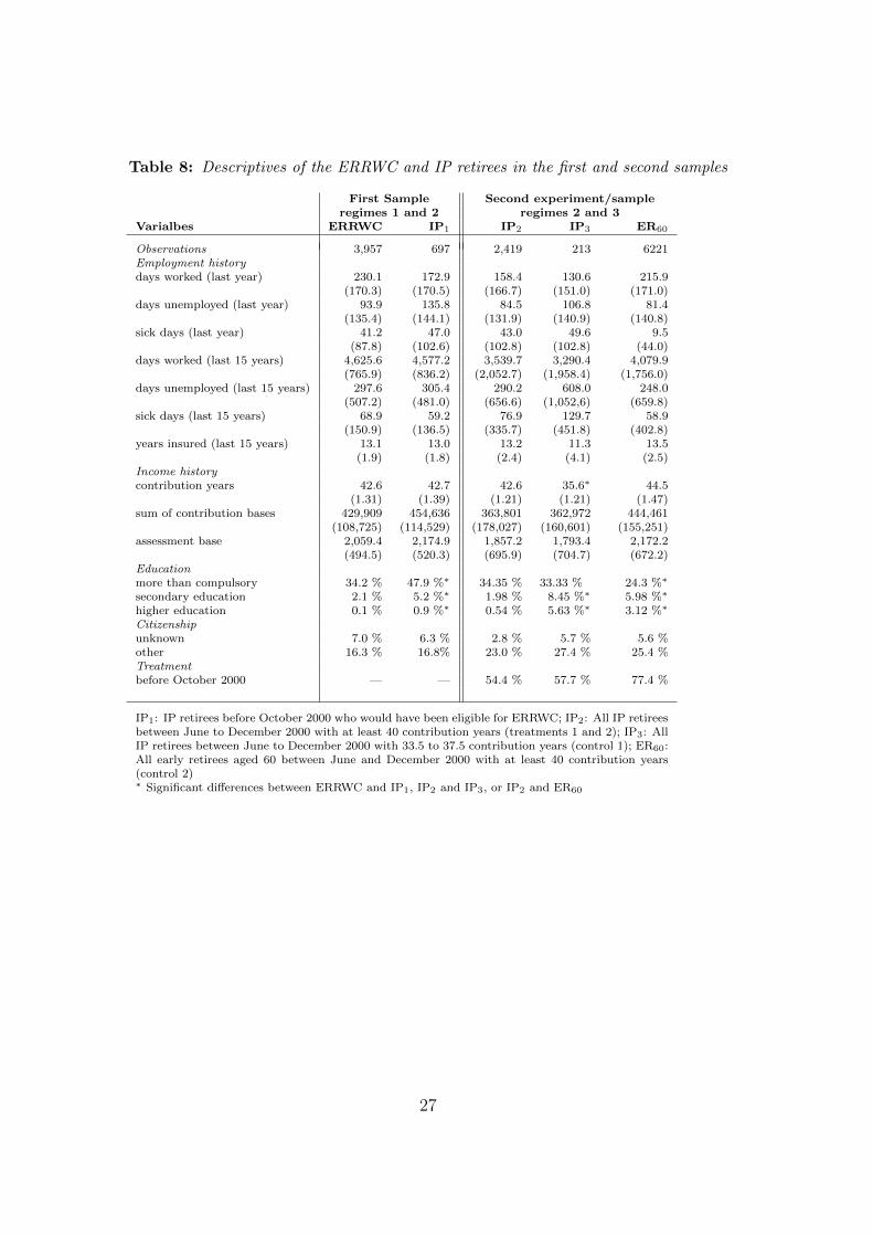
Table 8: Descriptives of the ERRWC and IP retirees in the first and second samples

First Sample Second experiment/sampleregimes 1 and 2 regimes 2 and 3

Varialbes ERRWC IP1 IP2 IP3 ER60

Observations 3,957 697 2,419 213 6221Employment historydays worked (last year) 230.1 172.9 158.4 130.6 215.9

(170.3) (170.5) (166.7) (151.0) (171.0)days unemployed (last year) 93.9 135.8 84.5 106.8 81.4

(135.4) (144.1) (131.9) (140.9) (140.8)sick days (last year) 41.2 47.0 43.0 49.6 9.5

(87.8) (102.6) (102.8) (102.8) (44.0)days worked (last 15 years) 4,625.6 4,577.2 3,539.7 3,290.4 4,079.9

(765.9) (836.2) (2,052.7) (1,958.4) (1,756.0)days unemployed (last 15 years) 297.6 305.4 290.2 608.0 248.0

(507.2) (481.0) (656.6) (1,052,6) (659.8)sick days (last 15 years) 68.9 59.2 76.9 129.7 58.9

(150.9) (136.5) (335.7) (451.8) (402.8)years insured (last 15 years) 13.1 13.0 13.2 11.3 13.5

(1.9) (1.8) (2.4) (4.1) (2.5)Income historycontribution years 42.6 42.7 42.6 35.6∗ 44.5

(1.31) (1.39) (1.21) (1.21) (1.47)sum of contribution bases 429,909 454,636 363,801 362,972 444,461

(108,725) (114,529) (178,027) (160,601) (155,251)assessment base 2,059.4 2,174.9 1,857.2 1,793.4 2,172.2

(494.5) (520.3) (695.9) (704.7) (672.2)Educationmore than compulsory 34.2 % 47.9 %∗ 34.35 % 33.33 % 24.3 %∗

secondary education 2.1 % 5.2 %∗ 1.98 % 8.45 %∗ 5.98 %∗

higher education 0.1 % 0.9 %∗ 0.54 % 5.63 %∗ 3.12 %∗

Citizenshipunknown 7.0 % 6.3 % 2.8 % 5.7 % 5.6 %other 16.3 % 16.8% 23.0 % 27.4 % 25.4 %Treatmentbefore October 2000 — — 54.4 % 57.7 % 77.4 %

IP1: IP retirees before October 2000 who would have been eligible for ERRWC; IP2: All IP retireesbetween June to December 2000 with at least 40 contribution years (treatments 1 and 2); IP3: AllIP retirees between June to December 2000 with 33.5 to 37.5 contribution years (control 1); ER60:All early retirees aged 60 between June and December 2000 with at least 40 contribution years(control 2)∗ Significant differences between ERRWC and IP1, IP2 and IP3, or IP2 and ER60

27

References

Adams, P., M.D. Hurd, D. McFadden, A. Merrill and T. Ribeiro (2003), ‘Healthy,

wealthy, and wise? tests for direct causal paths between health and socioeco-

nomic status’, Journal of Econometrics 112(1), 3–56.

Benzeval, M., J. Taylor and K. Judge (2000), ‘Evidence on the relationship be-

tween low income and poor health: is the government doing enough?’, Fiscal

Studies 21(3), 375–399.

Bloom, D.E. and D. Canning (2000), ‘The health and wealth of nations’, Science

287(5456), 1207–1209.

Case, A. (2001), ‘Does money protect health status? evidence from South African

pensions’, NBER Working Paper .

Cawley, J., J. Moran and S. Kosali (2010), ‘The impact of income on the weight

of elderly Americans’, Health Economics 19(8), 979–993.

Contoyannis, P., A.M. Jones and N. Rice (2004), ‘The dynamics of health in the

British Household Panel Survey’, Journal of Applied Econometrics 19(4), 473–

503.

Cutler, D., A. Deaton and A. Lleras-Muney (2006), ‘The determinants of mor-

tality’, The Journal of Economic Perspectives 20(3), 97–120.

Eurostat Statistics Database, Economic Policy Committee (2010), Expenditure

on pensions, Technical report, Eurostat.

URL: http: // epp. eurostat. ec. europa. eu/ tgm/ table. do? tab=

table&init= 1&language= en&pcode= tps00103

28

Frijters, P., J.P. Haisken-DeNew and M.A. Shields (2005), ‘The causal effect of

income on health: Evidence from German reunification’, Journal of Health

Economics 24(5), 997–1017.

Grossman, M. (1972), ‘On the Concept of Health Capital and the Demand for

Health’, Journal of Political Economy 80(2), 223–255.

Hauptverband der osterr. Sozialversicherungstrager (2010), ‘Statistisches Hand-

buch der osterreichischen Sozialversicherung 2010’.

Hofer, H. and R. Koman (2006), ‘Social security and retirement incentives in

Austria’, Empirica 33(5), 285–313.

Lindahl, M. (2005), ‘Estimating the effect of income on health and mortality

using lottery prizes as an exogenous source of variation in income’, Journal of

Human Resources 40(1), 144.

Manoli, D., K. Mullen, M. Wagner and C.C. Alberto (2009), ‘Pension Benefits &

Retirement Decisions: Income vs. Price Elasticities!’, mimeo .

Organisation for Economic Co-operation and Development (2005), Ageing and

Employment Policies: Austria, OECD Publishing, Paris.

Organisation for Economic Co-operation and Development (2006), Ageing and

Employment Policies: Live Longer, Work Longer, OECD Publishing, Paris.

Rogot, E., P.D. Sorlie and N.J. Johnson (1992), ‘Life expectancy by employment

status, income, and education in the National Longitudinal Mortality Study.’,

Public Health Reports 107(4), 457.

Smith, J.P. (1998), ‘Socioeconomic status and health’, The American Economic

Review 88(2), 192–196.

29

Smith, J.P. (1999), ‘Healthy bodies and thick wallets: The dual relation between

health and economic status’, The Journal of Economic Perspectives 13(2), 145–

166.

Statistik Austria (2011), ‘Jahrliche Sterbetafeln seit 1947 fur Osterreich. Official

mortality tables 1947–2008’.

URL: http: // www. statistik. at/ web_ de/ statistiken/

bevoelkerung/ demographische_ masszahlen/ sterbetafeln/

Thomas, D., E. Frankenberg, J. Friedman, J.-P. Habicht, M. Hakimi, N. Ingw-

ersen, Jaswadi, N. Jones, C. McKelvey, G. Pelto, B. Sikoki, T. Seeman, J.P.

Smith, C. Sumantri, W. Suriastini and S. Wilopo (2006), ‘Causal effect of

health on labor market outcomes: Experimental evidence’, UC Los Angeles:

California Center for Population Research .

Wu, S. (2003), ‘The effects of health events on the economic status of married

couples’, Journal of Human Resources 38(1), 219.

Zweimuller, J., R. Winter-Ebmer, R. Lalive, A. Kuhn, O. Ruf, S. Buchi and J.-

P. Wuellrich (2009), ‘The Austrian Social Security Database (ASSD)’. IEW

Working Paper, University of Zurich.

30