12

34

56

78

910

1112

13

Longitude

Latit

ude

−150 −100 −50 0 50 100 150

−50

050

●●

●●●

●

●

●●

●● ●

●

12

34

56

78

910

1112

13

Longitude

Latit

ude

−150 −100 −50 0 50 100 150

−50

050

●●

●

●

●

●

●

●

●

●

12

34

56

78

910

1112

13

Longitude

Latit

ude

−150 −100 −50 0 50 100 150

−50

050

●

●

●●●●

●

●●●●

●

12

34

56

78

910

1112

13

Longitude

Latit

ude

−150 −100 −50 0 50 100 150

−50

050

●

●

●

●

●

●

●

● ●●

Boreal winter Boreal spring

Boreal summer Boreal fall

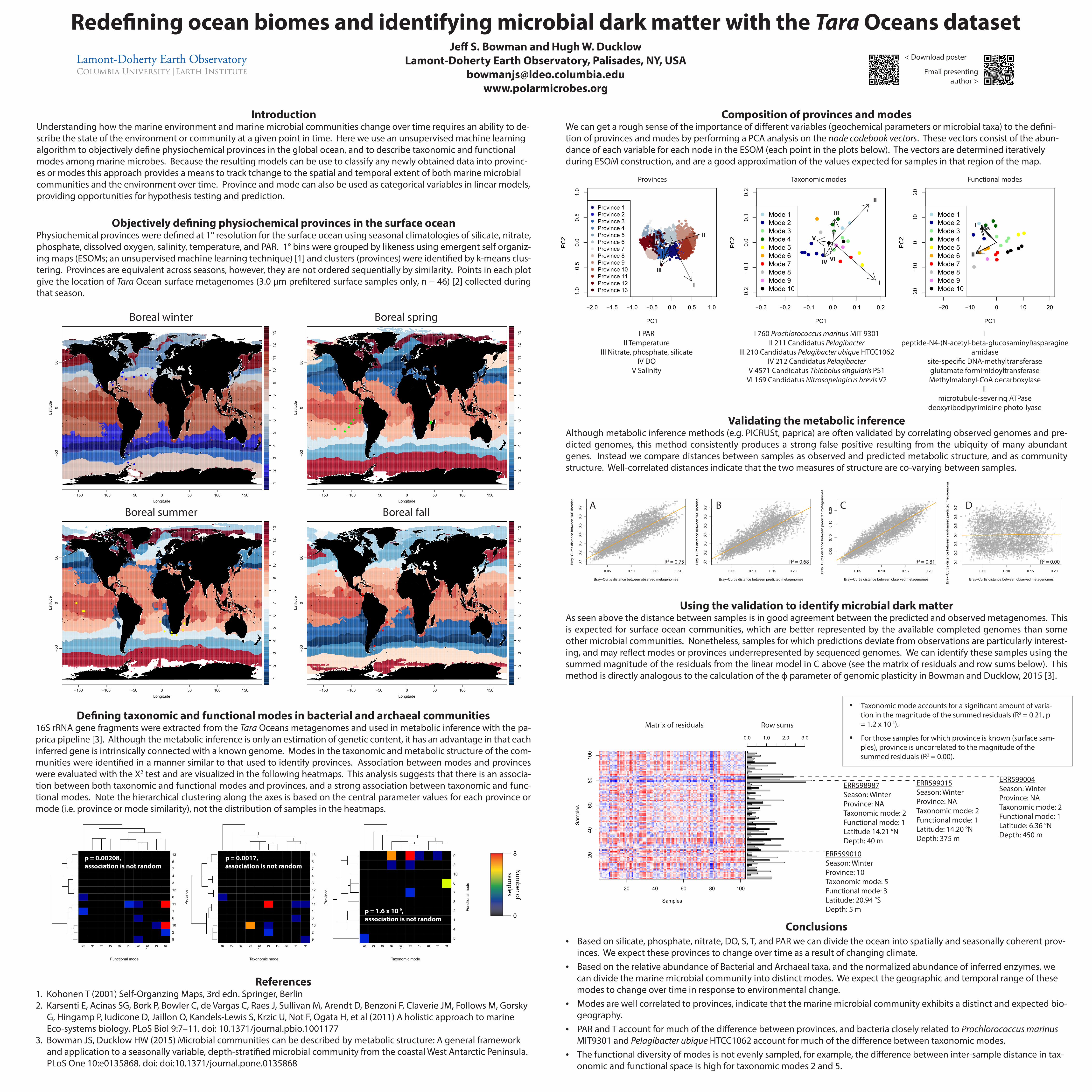
Objectively de�ning physiochemical provinces in the surface oceanPhysiochemical provinces were de�ned at 1° resolution for the surface ocean using seasonal climatologies of silicate, nitrate, phosphate, dissolved oxygen, salinity, temperature, and PAR. 1° bins were grouped by likeness using emergent self organiz-ing maps (ESOMs; an unsupervised machine learning technique) [1] and clusters (provinces) were identi�ed by k-means clus-tering. Provinces are equivalent across seasons, however, they are not ordered sequentially by similarity. Points in each plot give the location of Tara Ocean surface metagenomes (3.0 µm pre�ltered surface samples only, n = 46) [2] collected during that season.

De�ning taxonomic and functional modes in bacterial and archaeal communities16S rRNA gene fragments were extracted from the Tara Oceans metagenomes and used in metabolic inference with the pa-prica pipeline [3]. Although the metabolic inference is only an estimation of genetic content, it has an advantage in that each inferred gene is intrinsically connected with a known genome. Modes in the taxonomic and metabolic structure of the com-munities were identi�ed in a manner similar to that used to identify provinces. Association between modes and provinces were evaluated with the Х2 test and are visualized in the following heatmaps. This analysis suggests that there is an associa-tion between both taxonomic and functional modes and provinces, and a strong association between taxonomic and func-tional modes. Note the hierarchical clustering along the axes is based on the central parameter values for each province or mode (i.e. province or mode similarity), not the distribution of samples in the heatmaps.

IntroductionUnderstanding how the marine environment and marine microbial communities change over time requires an ability to de-scribe the state of the environment or community at a given point in time. Here we use an unsupervised machine learning algorithm to objectively de�ne physiochemical provinces in the global ocean, and to describe taxonomic and functional modes among marine microbes. Because the resulting models can be use to classify any newly obtained data into provinc-es or modes this approach provides a means to track tchange to the spatial and temporal extent of both marine microbial communities and the environment over time. Province and mode can also be used as categorical variables in linear models, providing opportunities for hypothesis testing and prediction.

Composition of provinces and modesWe can get a rough sense of the importance of di�erent variables (geochemical parameters or microbial taxa) to the de�ni-tion of provinces and modes by performing a PCA analysis on the node codebook vectors. These vectors consist of the abun-dance of each variable for each node in the ESOM (each point in the plots below). The vectors are determined iteratively during ESOM construction, and are a good approximation of the values expected for samples in that region of the map.

Validating the metabolic inferenceAlthough metabolic inference methods (e.g. PICRUSt, paprica) are often validated by correlating observed genomes and pre-dicted genomes, this method consistently produces a strong false positive resulting from the ubiquity of many abundant genes. Instead we compare distances between samples as observed and predicted metabolic structure, and as community structure. Well-correlated distances indicate that the two measures of structure are co-varying between samples.

Using the validation to identify microbial dark matterAs seen above the distance between samples is in good agreement between the predicted and observed metagenomes. This is expected for surface ocean communities, which are better represented by the available completed genomes than some other microbial communities. Nonetheless, samples for which predictions deviate from observations are particularly interest-ing, and may re�ect modes or provinces underrepresented by sequenced genomes. We can identify these samples using the summed magnitude of the residuals from the linear model in C above (see the matrix of residuals and row sums below). This method is directly analogous to the calculation of the ф parameter of genomic plasticity in Bowman and Ducklow, 2015 [3].

Conclusions• Based on silicate, phosphate, nitrate, DO, S, T, and PAR we can divide the ocean into spatially and seasonally coherent prov-

inces. We expect these provinces to change over time as a result of changing climate.• Based on the relative abundance of Bacterial and Archaeal taxa, and the normalized abundance of inferred enzymes, we

can divide the marine microbial community into distinct modes. We expect the geographic and temporal range of these modes to change over time in response to environmental change.

• Modes are well correlated to provinces, indicate that the marine microbial community exhibits a distinct and expected bio-geography.

• PAR and T account for much of the di�erence between provinces, and bacteria closely related to Prochlorococcus marinus MIT9301 and Pelagibacter ubique HTCC1062 account for much of the di�erence between taxonomic modes.

• The functional diversity of modes is not evenly sampled, for example, the di�erence between inter-sample distance in tax-onomic and functional space is high for taxonomic modes 2 and 5.

Rede�ning ocean biomes and identifying microbial dark matter with the Tara Oceans dataset

Je� S. Bowman and Hugh W. DucklowLamont-Doherty Earth Observatory, Palisades, NY, USA

bowmanjs@ldeo.columbia.eduwww.polarmicrobes.org

5 4 1 2 8 7 6 10 3 9

Functional mode

9

2

10

6

1

11

8

12

3

4

7

5

13

Prov

ince

6 2 8 5 10 3 7 9 1 4

Taxonomic mode

9

2

10

6

1

11

8

12

3

4

7

5

13

Prov

ince

p = 0.00208,association is not random

p = 0.0017,association is not random

8

0

Num

ber ofsam

ples

6 2 8 5 10 3 7 9 1 4

Taxonomic mode

5

4

1

2

8

7

6

10

3

9

Func

tiona

l mod

e

p = 1.6 x 10-9,association is not random

0.05 0.10 0.15 0.20

0.1

0.2

0.3

0.4

0.5

0.6

0.7

Bray−Curtis distance between observed metagenomes

Bray

−Cur

tis d

ista

nce

betw

een

rand

omiz

ed p

redi

cted

meg

agen

omes

0.05 0.10 0.15 0.20

0.05

0.10

0.15

0.20

Bray−Curtis distance between observed metagenomes

Bray

−Cur

tis d

ista

nce

betw

een

pred

icte

d m

etag

enom

es

0.05 0.10 0.15 0.20

0.1

0.2

0.3

0.4

0.5

0.6

0.7

Bray−Curtis distance between predicted metagenomes

Bray

−Cur

tis d

ista

nce

betw

een

16S

libra

ries

0.05 0.10 0.15 0.20

0.1

0.2

0.3

0.4

0.5

0.6

0.7

Bray−Curtis distance between observed metagenomes

Bray

−Cur

tis d

ista

nce

betw

een

16S

libra

ries

R2 = 0.68R2 = 0.75 R2 = 0.81 R2 = 0.00

A B C D

I PARII Temperature

III Nitrate, phosphate, silicateIV DO

V Salinity

I 760 Prochlorococcus marinus MIT 9301II 211 Candidatus Pelagibacter

III 210 Candidatus Pelagibacter ubique HTCC1062IV 212 Candidatus Pelagibacter

V 4571 Candidatus Thiobolus singularis PS1VI 169 Candidatus Nitrosopelagicus brevis V2

I peptide-N4-(N-acetyl-beta-glucosaminyl)asparagine

amidasesite-speci�c DNA-methyltransferaseglutamate formimidoyltransferaseMethylmalonyl-CoA decarboxylase

II microtubule-severing ATPase

deoxyribodipyrimidine photo-lyase

−0.3 −0.2 −0.1 0.0 0.1 0.2

−0.2

−0.1

0.0

0.1

0.2

PC1

PC2

●●

●● ●●●

●

●

●●

●

●

●

●

●

●

●●

●●

● ●● ●

●

●

●

●

●

●

●

●

●

●

Mode 1Mode 2Mode 3Mode 4Mode 5Mode 6Mode 7Mode 8Mode 9Mode 10

−20 −10 0 10 20

−20

−10

010

20

PC1

PC2

●●

●●

●●

●

●

●●●

●●

●●

●●●●

●

●

●●●

●

●

●

●

●

●

●

●

●

●

●

Mode 1Mode 2Mode 3Mode 4Mode 5Mode 6Mode 7Mode 8Mode 9Mode 10

−2.0 −1.5 −1.0 −0.5 0.0 0.5 1.0

−1.0

−0.5

0.0

0.5

1.0

PC1

PC2

●

●●●●

●● ●●●

● ●●●●

●●●● ●●●

● ●● ●●●

●

●●● ●

●

●

● ●●● ●●

●

●●●

●●●●●● ●●● ●●

●

●●●

●●

●●● ●●

●●●

●●

●

●●●●

●●

●

●

●●●●●●

●●●●

●●●●

●● ●

●

●

●●

●●

●

●●●●●●

●●

●●●●●

●●

●

●●●●

●●●●●●●●

●●●

●●●●●

●● ●

●●

●●

●●●●●

●●●

●●●

●●●

●●● ●●●●●

●●●●● ●

●

●●●●

●●●●

●●

●●

●●●●

● ●●●●●

●●●●

●●●● ●

●●●

●●●● ●● ● ●●

●●●

●●

●●●●●●●

●●●●

●●●●●●

●

●

● ●●●●

●●● ●●●●●●●●●●●●●●●●●●●●

●●●

●●

●●●●

●● ●●●●●● ●●●●

●●●●●●●●●●

●●●●●●●

●●●● ●●●●● ●●●●●●

●●●●

●●

●●

●●

●

● ●

● ●●●

●●●●

●●●●

●●●●●

●●●●●

●●●● ●

●●●●●

●●●●●●●

●●●●●● ●

●●●●●●●

● ●●●●●●●●●

●●●

●● ●● ●●●●●●

●●●●●●●●●●

●●● ●●●●

●● ●●

●●

●●●●

●●● ●

●●●●●

●●●

●●●●

●●

●

●

●●●●●

●●●●

●●●● ●

●●●

●

●●●

●●●●

●●

●●●●● ●●●

●●

●

●●

●●●●●●

●●●●●●●●

●●●● ●

●●●●●

●

●

● ●

●●

●

●●

●

●

●●

●

●

●

●

●

● ●● ●●

●

●●

●●●

●

●●

● ●

●●

●

●●

●●

●

●●●

●

●●●●

●●

●●

●●● ●●

●

●●●●

●

●●

●● ●●●●

●●●●

●● ●●

●●●●●

●●●●●

●●

●●●●

● ●●

●

●●

●

●●●● ●●●●

● ●● ●●

●●●●

●●●

●● ●

●

●

●●

●

●●

●●●

●●

●●

●

●

●● ●

●●

●

●

●

●

●●●●●●●●

●●●

●●●●●●●●●●●●●●●●●●●●●●●●●●●●●●●●●●●●●●●●●●●●●●●

●

●●●●●●●●●●●●●●●

●●●●●● ●●●●●●●●●●

●●●●●●●●●●●●●● ●●●●●

●●

●●

●●●●

●●

●●●

●●

●●

●

●●

●●

●

●

●●

●●

●

●

●●

● ●●●●

● ●

●●● ●●●

●●

●

●● ●●

●

●●●

●

●

●●●●● ●●

●

●● ●●

●

● ●●●●●●

●●

●●

●●

●● ●●●

●

●●●●

●

●●●●

●●● ● ●

●

●●●

●●●●

●● ●●●●

●●● ●●●●

●●

●● ● ●●●

●●●

●●●●

●●

●●

●●

●●●●●●

●●●●

●●

●●●●●●

●

●●●●●●●

●●

●

●●●●●

●●●●●●

●●●●●●

●●

●●●●●●

●●

●●●●●●●●●

●●●●●●●●●●●

●●●●● ●●●●●

● ●●●●●

●

●●

●

●●●●●●

●●

●●

●●●

●●

●●●●

●●●●●●●●●●●●

●

●●●●

●●● ●●

● ●●●●●●●

●

●●●●●●●

●●●●●●

●●

●●●●●●●●●●●●●●●

●●●●

●●●●●

●●●

●

●●

●●●●●●●●

●●●●●●

●●●●●●●●●●●●●●

●●●●●

●●●●●●●

●●●●●●●●●●●●●●●●●●

●●●●●●

●●

●

●●●●●●●

●●●●●●●●● ●●

●●●●

●●●●●●●●●●

●

●●●●●

●●●●●

●

●●●●●●●●●●●

●● ●●●

●●●

● ●●●●●

●● ●●

●●

●●●

●●●●●●

●●●●●●●●●●●

●●●●●●

●●●●

●●●●●●●●●●●

●● ●●

●●●●

●●●●

●●●●●●●●●●

●●

● ● ●●●●●●●●●

●●●●●

●●●●●●●●●

●

●

●●●●●●●●●●

●●

●●●●●

●●●

●●

●

●●●●●●●●

●

●

● ●●

●●●●●●●

●●●

●●●●●

●●●●

●

●●● ●

●

●

●●● ●●

●●●●● ●●●

●●●●●●●●●●●●●●

●●●●●●●●●●●●●●●●●●●●●●●●●●●●●

●●●●●●●●●●●●●●●

●●●●

●●●●●●●●

●●●●●●●●●

●●●●●●●●●●●

●

●●●●●●●●●

●●●●●●●● ●

●

●

●

●●●●●

●

●

●

●

●●

●●

●

●●

●●

●● ●

●●●

●

●●●●

●●

●●●●

●●●●

● ●●●

●

●●● ●

●

● ●

●●

●

●●

●

●

●

●

●

●

●

●

●

●

●

●

●

Province 1Province 2Province 3Province 4Province 5Province 6Province 7Province 8Province 9Province 10Province 11Province 12Province 13

IV

III

I

II

V

I

II

III

IV

V

VI

I

II

Provinces Taxonomic modes Functional modes

20 40 60 80 100

2040

6080

100

Samples

Sam

ples

0.0 1.0 2.0 3.0

ERR599015Season: WinterProvince: NATaxonomic mode: 2Functional mode: 1Latitude: 14.20 °NDepth: 375 m

ERR598987Season: WinterProvince: NATaxonomic mode: 2Functional mode: 1Latitude 14.21 °NDepth: 40 m

ERR599004Season: WinterProvince: NATaxonomic mode: 2Functional mode: 1Latitude: 6.36 °NDepth: 450 m

ERR599010Season: WinterProvince: 10Taxonomic mode: 5Functional mode: 3Latitude: 20.94 °SDepth: 5 m

• Taxonomic mode accounts for a signi�cant amount of varia-tion in the magnitude of the summed residuals (R2 = 0.21, p = 1.2 x 10-4).

• For those samples for which province is known (surface sam-ples), province is uncorrelated to the magnitude of the summed residuals (R2 = 0.00).

Matrix of residuals Row sums

References1. Kohonen T (2001) Self-Organzing Maps, 3rd edn. Springer, Berlin2. Karsenti E, Acinas SG, Bork P, Bowler C, de Vargas C, Raes J, Sullivan M, Arendt D, Benzoni F, Claverie JM, Follows M, Gorsky

G, Hingamp P, Iudicone D, Jaillon O, Kandels-Lewis S, Krzic U, Not F, Ogata H, et al (2011) A holistic approach to marine Eco-systems biology. PLoS Biol 9:7–11. doi: 10.1371/journal.pbio.1001177

3. Bowman JS, Ducklow HW (2015) Microbial communities can be described by metabolic structure: A general framework and application to a seasonally variable, depth-strati�ed microbial community from the coastal West Antarctic Peninsula. PLoS One 10:e0135868. doi: doi:10.1371/journal.pone.0135868

< Download poster

Email presenting author >