Helsinki University of Technology

Department of Biomedical Engineering and Computational Science Publications

Teknillisen korkeakoulun Lääketieteellisen tekniikan ja laskennallisen tieteen laitoksen julkaisuja

October, 2008 REPORT A05

BOUNDARY ELEMENT METHOD IN SPATIAL

CHARACTERIZATION OF THE ELECTROCARDIOGRAM

Matti Stenroos

Helsinki University of Technology

Faculty of Information and Natural Sciences

Department of Biomedical Engineering and Computational Science

Teknillinen korkeakoulu

Informaatio- ja luonnontieteiden tiedekunta

Lääketieteellisen tekniikan ja laskennallisen tieteen laitos

Dissertation for the degree of Doctor of Science in Technology to be presented with due permission of the

Faculty of Information and Natural Sciences, Helsinki University of Technology, for public examination

and debate in Auditorium E at Helsinki University of Technology (Espoo, Finland) on the 25th of October,

2008, at 12 o'clock noon.

Distribution:

Helsinki University of Technology

Department of Biomedical Engineering and Computational Science

http://www.becs.tkk.fi

P.O.Box 2200

FI-02015 TKK

FINLAND

Tel. +358 9 451 3172

Fax +358 9 451 3182

E-mail: matti.stenroos@tkk.fi

© Matti Stenroos

ISBN 978-951-22-9586-9 (printed)

ISBN 978-951-22-9587-6 (PDF)

ISSN 1797-3996

Picaset Oy

Helsinki 2008

Abstract

The electrochemical activity of the heart gives rise to an electric field. Inelectrocardiography, cardiac electrical activity is assessed by analyzing thepotential distribution of this field on the body surface. The potential dis-tribution, or the set of measured surface-voltage signals, is called the elec-trocardiogram (ECG). Spatial properties of the ECG can be captured withbody surface potential mapping (BSPM), in which the electrocardiogram ismeasured using dozens of electrodes. In this Thesis, methods for solvingthe forward and inverse problems of electrocardiography are developed andapplied to characterization of acute myocardial ischemia.

The methodology is based on numerical computation of quasi-static electricfields in a volume conductor model. An open-source Matlab toolbox for solv-ing volume conductor problems with the boundary element method (BEM)is presented. The Galerkin BEM and analytical operator-integrals are, forthe first time, applied to the epicardial potential problem; the formulation fora piece-wise homogeneous volume conductor is presented in detail, enablingstraightforward inclusion of the lungs or other inhomogeneities in the thoraxmodel.

The results show that errors due to discretization and forward-computationare smaller with the linear Galerkin (LG) method than with the conventionalmethods. These benefits do, however, not reflect to the Tikhonov-regularizedinverse solution. If the lungs are omitted, as commonly is done, the choiceof the computational method is not significant.

In a set of 22 patients measured with BSPM during coronary angioplasty(PTCA), the application of a BEM thorax model with dipolar equivalentsources enabled accurate discrimination between occluded coronary arteries:the correct classification was obtained in 21 patients using the BSPM and in20 patients using a 5-electrode set suggested elsewhere. The ischemic regionscould also be localized anatomically correctly with simplified epicardial po-tential imaging, even though patient-specific thorax models were not used. Inanother set, comprising 79 acute ischemic patients and 84 controls, dipole-markers performed well in detection and quantification of acute ischemia.These results show that the modeling-approach can provide valuable infor-mation also without patient-specific models and complicated protocols.

Tiivistelma

Sydanlihassolujen sahkokemiallinen toiminta synnyttaa sahkokentan. Elek-trokardiografiassa sydamen sahkoista toimintaa tutkitaan analysoimalla ta-man kentan potentiaalijakaumaa kehon pinnalla. Kehon pintapotentiaalija-kaumaa tai siita mitattua signaalijoukkoa kutsutaan elektrokardiogrammiksi(EKG). Elektrokardiogrammin spatiaaliset piirteet saadaan taltioitua EKG-kartoituksessa, jossa elektrokardiogrammia mitataan kymmenien elektrodienavulla. Tassa vaitoskirjassa kehitetaan kentanlaskentamenetelmia elektrokar-diografian suoran ja kaanteisen ongelman ratkaisuun. Menetelmia sovelletaanakuutin sydanlihasiskemian karakterisointiin.

Tyon metodiikka perustuu kvasistaattisten sahkokenttien numeeriseen las-kentaan rintakehan johtavuusmallissa reunaelementtimenetelman (BEM) avul-la. BEM-perustyokaluista on koottu avoimen lahdekoodin Matlab-kirjasto.Galerkinin painotusta ja analyyttisesti laskettuja operaattori-integraaleja so-velletaan ensimmaista kertaa epikardiaalipotentiaalin reunaelementtiratkai-sussa. Tarvittavien yhtaloiden johto ja diskretointi paloittain jatkuvassa va-liaineessa esitetaan perusteellisesti, mika mahdollistaa keuhkojen suoraviivai-sen sisallyttamisen rintakehamalliin.

Lineaarinen Galerkin-menetelma pienentaa suoran ongelman laskennan jadiskretoinnin aiheuttamia virheita verrattattuna yleisesti kaytettyyn kollo-kaatiomenetelmaan. Nama hyodyt eivat kuitenkaan heijastu Tikhonov-regu-larisoinnin avulla laskettuihin kaanteisen ongelman ratkaisuihin. Jos keuhkotjatetaan mallintamatta, kuten alan tutkimuksessa tapana on, laskentamene-telman valinnalla ei ole merkitysta.

Sepelvaltimon pallolaajennuksen aikana mitattujen EKG-kartoitusten aineis-tossa tukkeutunut valtimo kyettiin tunnistamaan BEM-rintakehamallin jadipolimallinnuksen avulla: 22 potilaasta 21 luokiteltiin oikein EKG-kartoi-tuksen ja 20 eraan aiemmin kuvaillun viiden elektrodin joukon avulla. Iskee-miset alueet paikannettiin yksinkertaistetun epikardiaalipotentiaalikuvanta-misen avulla anatomisesti oikein — ilman potilaskohtaisia rintakehamalleja.79 iskemiapotilaasta ja 84 terveesta verrokista koostuvassa aineistossa dipoli-malli tuotti lupaavia tuloksia sydanlihasiskemian havaitsemisessa ja infarkti-vaurion koon arvioinnissa. Tulokset osoittavat, etta kentanlaskennallinen la-hestymistapa tuottaa hyodyllista tietoa myos ilman potilaskohtaisia mallejaja monimutkaisia menetelmia.

Contents

Preface ix

List of Publications xi

Summary of Publications xiii

Author’s Contribution xiv

List of Abbreviations xv

1 Introduction 1

1.1 Aims and Outline . . . . . . . . . . . . . . . . . . . . . . . . . 2

2 Volume Conductor Modeling 5

2.1 Quasi-Static Approximation of Bioelectric Fields . . . . . . . . 5

2.2 Boundary Element Method . . . . . . . . . . . . . . . . . . . . 9

2.3 Surface Integral Equations for Electric Potential . . . . . . . . 10

3 Forward and Inverse Problems of Electrocardiography 17

3.1 Source Modeling . . . . . . . . . . . . . . . . . . . . . . . . . 17

3.2 Epicardial Potential Imaging . . . . . . . . . . . . . . . . . . . 23

4 Detection and Localization of Myocardial Ischemia 29

4.1 Myocardial Ischemia and the Electrocardiogram . . . . . . . . 29

4.2 Datasets and Preprocessing . . . . . . . . . . . . . . . . . . . 30

4.3 Dipole Modeling . . . . . . . . . . . . . . . . . . . . . . . . . 32

4.4 Epicardial Potential Imaging . . . . . . . . . . . . . . . . . . . 37

5 Summary and Outlook 43

References 45

Preface

The research reported in this Thesis was carried out in the cardiac researchgroup of the Laboratory of Biomedical Engineering and Department of Bio-medical Engineering and Computational Science (BECS) at Helsinki Univer-sity of Technology.

I have been lucky to have an assistant-post in the laboratory, having a lot ofscientific freedom, interesting teaching-tasks, and a stable source of income. Iwish to thank my bosses & supervisors, Topi Katila and Risto Ilmoniemi, forthis opportunity and their continuous interest in my work. Jukka Nenonenhas been my mentor for years; I thank him for all his advice and good com-pany. Collaboration with Jens Haueisen and his research group from Jena,Germany, has been both fruitful and fun—Vielen Dank! Of teachers at theuniversity, I wish to thank Jukka Sarvas for in-depth discussions and excellentcourses on computational electromagnetism.

A part of this work has been carried out in collaboration with the Divi-sion of Cardiology at Helsinki University Central Hospital (HUCH). Thecardiology-team has been our essential link to the clinical world, buildingbridges between the clinical and theoretical worlds of electrocardiographywith us. Hence I wish to thank our clinical colleagues Lauri Toivonen,Markku Makijarvi, Helena Hanninen, Paula Vesterinen, Ilkka Tierala, andMinna Kylmala, for the fruitful collaboration.

The cardiac group of our laboratory has been a great base for my research:relaxed atmosphere, stimulating discussions, nice working-environment. Forthese I am grateful to my current and former colleagues; Heikki Vaananen,Mats Lindholm, Teijo Konttila, Juhani Dabek, and Kim Simelius at ourdepartment, and Juha Montonen and Ville Mantynen at the Biomag Lab-oratory, HUCH. I also wish to thank other people at our department foratmosphere and discussions—especially Ari Koskelainen, Pekka Merilainen,and Mika Pollari. In addition, I thank Uwe Steinhoff from PTB Berlin forgood company and providing me with a peaceful office in Berlin.

This Thesis was pre-examined by Jari Hyttinen, Tampere University of Tech-nology, and Rob MacLeod, University of Utah, USA. I am grateful to themfor their thorough commentaries that helped me improve the Thesis manu-script.

During the research presented in this Thesis, I have received additional fund-

ix

ing from the Foundation of Technology in Finland, Academy of Finland, andgraduate school“Functional Research in Medicine”; I thank these institutionsfor their support.

I wish to thank my friends for their company during bicycle rides, pubevenings, music sessions, and many other out-of-office activities. I am alsograteful to my parents and my sister for their support. Finally, I thank Lindafor her love and for our happy life.

Espoo, October 2008

Matti Stenroos

x

List of Publications

This Thesis consists of an overview and the following six Publications.

I. M. Stenroos, V. Mantynen, and J. Nenonen. A Matlab Library forSolving Quasi-Static Volume Conduction Problems Using the BoundaryElement Method. Computer Methods and Programs in Biomedicine,88:256–263, 2007. c©2007 Elsevier.

II. M. Stenroos and J. Haueisen. Boundary Element Computations in theForward and Inverse Problem of Electrocardiography: Comparison ofCollocation and Galerkin Weightings. IEEE Transactions on Biomed-ical Engineering, 55:2124–2133, 2008. c©2008 IEEE.

III. M. Stenroos. Transfer Matrix for Epicardial Potential in a Piece-WiseHomogeneous Thorax Model: the Boundary Element Formulation. De-partment of Biomedical Engineering and Computational Science Pub-lications, Report A04, 9 pages, 2008.

IV. M. Stenroos, M. Lindholm, H. Hanninen, I. Tierala, H. Vaananen,and T. Katila. Dipole Modeling in Electrocardiographic Classificationof Acute Ischemia. Computers in Cardiology 2005, 32:655–658, 2005.c©2005 IEEE.

V. M. Stenroos, M. Lindholm, P. Vesterinen, M. Kylmala, T. Konttila, J.Dabek, and H. Vaananen. Electrocardiographic Detection and Quan-tification of Acute Myocardial Ischemia with Dipole Modeling. Com-puters in Cardiology 2006, 33:29–32, 2006.

VI. M. Stenroos, H. Hanninen, M. Lindholm, I. Tierala, and T. Katila.Lead Field Formulation for Epicardial Potential in ElectrocardiographicLocalization of Acute Myocardial Ischemia. IFMBE Proceedings, 11:2265-1–2265-5, 2005. c©2005 EMBEC’05 & IFMBE.

Copyrighted Publications are reproduced with permission.

xi

Summary of Publications

I. A Matlab Library for Solving Quasi-Static Volume Conduc-tion Problems Using the Boundary Element MethodBasic principles of the boundary element method (BEM) are reviewed,and BEM discretization of quasi-static electric potential and biomag-netic volume conduction problems is presented. A Matlab library forsolving these problems is described, validated, and applied to variousproblems. The library is the first free, open-source toolbox for solvingthis kind of problems with the BEM using the Matlab environment. Itis currently in use in over 20 foreign research groups.

II. Boundary Element Computations in the Forward and InverseProblem of Electrocardiography: Comparison of Collocationand Galerkin WeightingsSource-modeling and epicardial potential problems are presented withhelp of single- and double-layer operators and discretized with both col-location and Galerkin BEMs. In the epicardial potential problem, theGalerkin BEM is presented and analytical operator integrals are usedfor the first time. The linear Galerkin method yields the smallest errorsin discretization and forward computation of the epicardial potential.In the inverse solution, the modeling of lungs has clearly larger effecton results than the choice of the BEM technique does.

III. Transfer Matrix for Epicardial Potential in a Piece-Wise Ho-mogeneous Thorax Model: the Boundary Element FormulationThe integral equation system relating the epicardial and body surfacepotentials in a piece-wise homogeneous thorax model is derived. Theequations are presented in terms of single- and double-layer operators,and discretization is done with both collocation and Galerkin BEMs.The derivation is more compact and general and the resulting transfermatrix is mathematically more stable than those in earlier studies.

IV. Dipole Modeling in Electrocardiographic Classification of AcuteIschemiaA BEM volume conductor model and dipolar equivalent sources are ap-plied to spatial characterization of the electrocardiogram. The datasetconsists of body surface potential mappings (BSPM) measured from 22patients during coronary angioplasty operations, classified according tothe occluded coronary artery. Up to 21 of the 22 patients could beclassified to the correct category by comparing the dipole directions.

xiii

V. Electrocardiographic Detection and Quantification of AcuteMyocardial Ischemia with Dipole ModelingThe BEM and dipole models are used in detection and size estimation ofacute myocardial ischemia. Dipoles are fitted to electrocardiographicmarkers derived from the BSPM data of 79 patients and 84 healthycontrols. Various parameters are derived from the dipole vectors. Then,receiver-operating-characteristic curves are used for finding the best-discriminating markers between the patients and controls, and markersproviding the best correlations with the CK-Mb mass are sought for.

VI. Lead Field Formulation for Epicardial Potential in Electrocar-diographic Localization of Acute Myocardial IschemiaEpicardial potential imaging is applied to localization of the ischemicregion from the same dataset that was used in Publication IV. A sim-ple template-based method is presented; the method provides for robustsearching of the center of the ischemic region. Localization results areanatomically correct. This study won the first price in the IFMBEYoung Investigator Competition of the EMBEC’05 conference.

Author’s Contribution

The author of this Thesis (“the author”) was the main investigator and prin-cipal writer in all included Publications. The theoretical work and computerprogramming related to the boundary element method was mainly carriedout by the author; only the numerical integration rules and tools for analyt-ical validation were implemented by others.

In Publication I, the author designed and implemented the BEM libraryand examples, while co-authors performed the validation. In PublicationII, the author developed and implemented all computational models andtest scenarios; results were interpreted together with the co-author, who alsocontributed to the study design. In Publications IV–VI, co-authors collected,documented and preprocessed the patient data; the author developed andapplied the computational models and analyzed the results.

All Publications were written by the author. Co-authors contributed byreviewing the manuscripts.

xiv

List of Abbreviations

ATI Activation time imagingBEM Boundary element methodBSPM Body surface potential mappingDOF Degree of freedomECD Equivalent current dipoleEDL Equivalent double-layerECG Electrocardiogram or electrocardiographyFEM Finite element methodCC Constant collocation methodCG Constant Galerkin methodLC Linear collocation methodLG Linear Galerkin methodRE Relative errorSMD Single moving dipoleTMP Transmembrane potentialUDL Uniform double-layer

xv

1 Introduction

Electrochemical activity of cardiac muscle cells gives rise to electric and mag-netic fields [1]. The electric field is reflected on the body surface as a potentialdistribution. In electrocardiography, cardiac electrical activity is assessed bystudying voltage signals measured on the body surface. The set of measuredsignals, or more generally, the body surface potential distribution, is calledthe electrocardiogram (ECG).

In clinical use, the most common electrocardiographic application is the 12-lead ECG [2], which is measured with nine electrodes. The 12-lead ECG isvisualized as a set of time-voltage tracings, and spatial analysis is carried outby comparing relative amplitudes of the tracings. From the 12-lead ECG,one can characterize the cardiac rhythm and infer the approximate locationand propagation direction of the mean cardiac electrical activity.

In body surface potential mapping (BSPM), the ECG is measured with tensof electrodes, yielding a more accurate spatial sampling of the potential dis-tribution on the thorax than that in the 12-lead ECG. The BSPM data arecommonly processed as multi-lead ECG, a collection of time-voltage trac-ings; quantitative analysis is based on features that are extracted from singleleads, while the spatial analysis resides typically on qualitative level, suchas visual inspection of the spatial distributions of the single-lead features.With this kind of analysis, geometrical properties of potential distributionsand the knowledge of electrode positions are not effectively utilized. Overall,the large dimension of the BSPM data poses a challenge for the analysis.

Challenges of the BSPM analysis are tackled with modeling-approaches, inwhich the relationship between the cardiac electrical activity and the result-ing ECG is characterized. In these approaches, the cardiac electrical activityis represented either with help of a mathematical source model or in terms ofepicardial potential. Electrical properties of the thorax are modeled applyinganatomical imaging, image processing, electromagnetic theory, and numeri-cal mathematics. Computation of the ECG from a known source model orepicardial potential is commonly referred to as the forward problem of electro-cardiography. Respectively, estimation of the sources or epicardial potentialfrom measured ECG data is called the inverse problem of electrocardiogra-phy.

The anatomical information needed in the model building is obtained with,e.g., magnetic resonance imaging or X-ray computed tomography. Electri-

1

cal properties of the thorax are typically assumed piece-wise homogeneous,enabling application of the boundary element method (BEM) in the numer-ical computations. In order to obtain accurate results, the anatomical andcomputational models need to be constructed individually for each patient; inaddition to imaging and computing facilities, lots of manual work from skilledpeople is thus needed. The modeling approaches are hereby used primarilyfor research purposes. Overall, the worlds of clinical electrocardiography andmodeling are wide apart.

1.1 Aims and Outline

The primary aim of this Thesis is to develop computational methods andcomputer program libraries for solving the electrocardiographic forward andinverse problems. The method development is focused on boundary elementmodeling of the epicardial potential problem.

The secondary aim is to bring simple modeling-approaches of electrocardio-graphy a step closer to the clinical world; to show that modeling can yieldvaluable information also without individual thorax models, exactly localizedelectrodes, and complicated analysis protocols.

This Thesis consists of an overview and six Publications. In the overview,the principal aim is to wrap the theory presented in Publications I-III into acompact but thorough package, presenting the source-modeling and epicar-dial potential problems in the same context and notation for the first time.The overview provides also more background for and some discussion onPublications II and III and an introduction on source-modeling methods. Inaddition, the methodology and results of Publications IV-VI are summarized,extended, and briefly discussed.

The overview is organized as follows:

• Chapter 2: The quasi-static approximation of bioelectromagnetic fieldsis reviewed, and the principle behind the boundary element method(BEM) is introduced. Computation of electric potential in a volumeconductor using the BEM is presented in a compact, but thoroughmanner.

• Chapter 3: Forward and inverse problems of electrocardiography arereviewed: Principles and methodology of source-modeling are intro-

2

duced, linking to the theory presented in Chapter 2. Epicardial po-tential imaging is reviewed in more detail; computational methods andvolume conductor modeling are treated. As part of the review, the Pub-lications II and III in epicardial potential imaging and Publications IVand V in dipole modeling are placed in the proper context.

• Chapter 4: Methods treated in this work are applied to spatial chara-terization of myocardial ischemia. First, dipole modeling is appliedto detection, coarse localization, and quantification of myocardial is-chemia. Then, simplified epicardial potential imaging is used in local-ization of the ischemic region.

• Chapter 5: a summary of and outlook on this Thesis and its mainresults is given.

3

2 Volume Conductor Modeling

2.1 Quasi-Static Approximation of Bioelectric Fields

2.1.1 Wave Equations for Potentials

Electromagnetic phenomena are characterized with the Maxwell equations[3]. An electrically active nerve or muscle cell acts as a source of electro-motive force that gives rise to electric field and current in the extracellulardomain. In macroscopic scale, the sources of these fields can be modeled interms of primary charge density ρp and current density �Jp [1]. Biologicalmedium is non-magnetic, conductive, and, at bioelectrical field strengths,electrically linear. With these source and material properties and harmonictime dependency of angular frequency ω, the Maxwell equations are

∇ · �E =ρp

ε(1)

∇ · �B = 0 (2)

∇× �E = iω �B (3)

∇× �B = μ0�Jp + μ0(σ − iωε) �E, (4)

where �E is the electric field, �B is the magnetic induction field, ε and σ are thepermittivity and conductivity of the medium, μ0 is the magnetic permeabilityof vacuum, and i is the complex unit: i =

√−1. The relationship betweenthe primary charges and currents in homogeneous medium is obtained bytaking divergence of Eq. 4 and applying Eq. 1, yielding

ρp

ε=

∇ · �Jp

iωε − σ. (5)

In electrocardiography, we are interested in voltages—potential-differences.Hereby it is logical to characterize the cardiac electromagnetic field withpotential-functions. From Eqs. 2 and 3, we get expressions for fields in termsof vector potential �A and scalar potential φ:

�B = ∇× �A (6)

�E = iω �A −∇φ. (7)

Using these relations in Eqs. 1 and 2 and applying the Lorenz gauge [3] giveswave equations for potentials. The general solutions of these equations are

5

obtained by integrating the source density weighted with the Green functionof the wave equation, leading to [4]

�A =μ0

4π

∫Vp

�Jpeik|�r−�r ′|

|�r − �r ′| dV ′ (8)

φ =1

4π(iωε − σ)

∫Vp

(∇ ′ · �Jp)eik|�r−�r ′|

|�r − �r ′| dV ′, (9)

where

k2 = ω2μ0ε(1 +

iσ

ωε

), (10)

�r and �r ′ are position vectors in field and source spaces, respectively, and Vp

is the volume containing all primary sources.

In Eq. 4, there are three types of currents: the primary currents �Jp, resistive

volume currents σ �E, and displacement currents iωε �E. The relative strengthof displacement1 and resistive currents is characterized by the ratio ωε/σ.This ratio defines, whether the medium acts primarily as a conductor or asan insulator, and, whether the wave motion is decaying or propagating. Thestrength of the inductive coupling in Eq. 3 is also governed by σ, ε, and ω.

2.1.2 Electrical Properties of Biological Tissues

Electrical properties of biological tissue depend on frequency and tissue type.In some tissues, e.g. muscles, these parameters are also anisotropic due to thedirected fibrous structures. Tissue conductivity at frequencies below 1 kHzhas been studied, e.g., in [5–8]. Capacitive properties at low frequencies have,to the author’s knowledge, been studied only by Schwan and Kay [9,10] andGabriel et al. [8]. Values for permittivity ε, conductivity σ, and the amplituderatio of displacement and resistive currents in various tissue types at threefrequencies are given in Table 1. The conductivities reported by Gabriel etal. were, in general, lower than those reported by Schwan and Kay.

Measurement of permittivity at low frequencies is prone to errors. The mainsource of error is polarization that takes place at the electrode–tissue interface[8, 9]. In Table 1, the values marked with asterisk are upper-limit values:in [10] it is written that “The values at 10 cps are possibly 3 to 10 timessmaller than quoted”. According to Gabriel et al. [8], electrode polarization

1Effects of the displacement currents on the bioelectromagnetic fields are commonlyreferred to as “capacitive effects”.

6

Table 1: Electrical properties of biological tissues [8, 10]. The values markedwith asterisk are upper-limit estimates.

10 Hz Schwan and Kay Gabriel et al.ε/106ε0 σ (S/m) |ωε/σ| εr/106 σ (S/m) |ωε/σ|

Heart 20∗ 0.10 0.100∗ 23 0.06 0.233Liver 50∗ 0.12 0.200∗ 20 0.03 0.371Lung 25∗ 0.09 0.150∗ 30 0.03 0.596

Muscle 30∗ 0.10 0.150∗ 60 0.23 0.148

100 HzHeart 0.82 0.09 0.040 4.00 0.09 0.247Liver 0.85 0.13 0.035 0.90 0.04 0.125Lung 0.45 0.09 0.025 1.50 0.05 0.167

Muscle 0.80 0.11 0.035 18.50 0.34 0.303

1000 HzHeart 0.32 0.12 0.150 0.30 0.11 0.152Liver 0.15 0.13 0.060 0.08 0.04 0.111Lung 0.09 0.10 0.050 0.10 0.05 0.111

Muscle 0.13 0.12 0.060 0.65 0.45 0.080

may affect their results below 100 Hz by a factor of two or three. Thesemeasurements and results are discussed in more detail in [11].

2.1.3 Quasi-Static Approximation

The wave motion is characterized by the exponential term in Eqs. 8 and 9.Applying the Taylor expansion,

eik|�r−�r ′| = 1 + ik|�r − �r ′| − (k|�r − �r ′|)2

2!+ ... (11)

Studying the magnitude of k with values from Table 1, we see that

|k||�r − �r ′| =

∣∣∣∣∣∣ω√

μ0ε

√1 +

iσ

ωε

∣∣∣∣∣∣ |�r − �r ′| (12)

< 0.002, f = 10 Hz

< 0.001, f = 100 Hz

< 0.017, f = 1000 Hz.

7

Hence we can approximate that, at frequencies below 100 Hz, eik|�r−�r ′| = 1.This means that a change in the source distribution is assumed to reflectinstantaneously into all field points. At higher frequencies, this assumptionintroduces small errors.

The electric field is calculated from potentials according to Eq. 7, where iω �Acorresponds to the inductive component of the field. The relative strength ofinductive effects can be studied by calculating the ratio of ω �A and ∇φ for adifferential source element [4, 11]. Such a calculation leads to

|ωA||∇φ| ≈ (|k||�r − �r ′|)2. (13)

The inductive effects can thus safely be omitted. The electric field can thenbe calculated from the scalar potential: �E = −∇φ.

According to the ratios presented in Table 1, resistive currents dominateover the displacement currents: Gabriel et al. reported [8] that ωε/σ is atelectrocardiographic frequencies larger than 0.1. Both Schwan and Kay [10]and Gabriel et al. reported ratios of over 0.15 at 10 Hz, but these resultsare unreliable. On basis of these results, it is not clear, whether biologicaltissues can be assumed purely resistive at bioelectric frequencies. As faras the author of this Thesis knows, the error introduced by omitting thedisplacement currents has not been studied in detail. In [12], the validity ofthis approximation was studied using a multi-layer spherical model. In thatstudy, however, only small (ωε/σ <= 0.004) or large (ωε/σ ≈ 1) ratios weretested. With the smaller ratio, there were no noticeable capacitive effects;with the larger ratio, the effects were clear. Henceworth, this study is basedon the conventional assumption that capacitive effects are so small that theycan be left out of the calculations without introducing major errors.

When propagative, inductive, and capacitive effects are omitted, the Maxwellequations are simplified to the static form. Because the sources are still time-dependent and conductivity may possess frequency dependency, the concept”quasi-static” is used. The conductivity is commonly assumed independentof the frequency, following the results of [6]. In practice, this means that tis-sues are not supposed to act as temporal filters. To the author’s knowledge,the error introduced by this assumption on common electrocardiographic ap-plications has not been studied; in [12], it was concluded that the frequencydependency of the conductivity may act as a temporal filter on the electroen-cephalogram and that capacitive effects due to vernix caseosa affect the fetalelectrocardiogram.

8

In summary, the quasi-static Maxwell equations for conductive, non-magnetic,electrically linear material are

∇ · �E =ρp

ε(14)

∇ · �B = 0 (15)

∇× �E = 0 (16)

∇× �B = μ0( �Jp + σ �E). (17)

Taking divergence of Eq. 17 and applying �E = −∇φ yields the Poissonequation in terms of primary-current sources:

∇ · (σ∇φ) = ∇ · �Jp. (18)

2.2 Boundary Element Method

The boundary element method is mathematically based on the method ofweighted residuals [13]: Consider the problem

L[f ](�r) = g(�r), (19)

where L is a differential or integral operator, g is a known function, and fis the unknown function that L acts on. First, approximate f as a linearcombination of N basis functions ψj(�r) and insert the approximation to theoriginal equation:

f(�r) ≈N∑

j=1

ϕjψj(�r) (20)

⇒N∑

j=1

ϕjL[ψj](�r) − g(�r) = RN(�r), (21)

where RN is the residual of the approximated solution. Then, force theresidual to zero with respect to N weight functions wi(�r) over the solutiondomain Ω: ∫

ΩRN(�r)wi(�r)dΩ = 0 (22)

⇒N∑

j=1

ϕj

∫Ω

wi(�r)L[ψj](�r)dΩ =∫Ω

wi(�r)g(�r)dΩ. (23)

9

Now the discretized problem can be written in matrix form:

LΦ = g, (24)

where Φ and g are N × 1–vector with elements ϕi and gi =∫Ω wi(�r)g(�r)dΩ,

respectively, and L is an N × N matrix with elements

Lij =∫Ω

wi(�r)L[ψj](�r)dΩ. (25)

The coefficients ϕj are, in principle, solved from Eq. 24 by inverting thematrix L.

The most simple choice for the weight function is the Dirac δ function. Withthis choice, the error is minimized in a discrete set of points [13]. This ap-proach is called the point collocation method, and the definition points of theδ functions are referred to as the collocation points. The collocation methodprovides for a computationally efficient solution of the residual-minimizationproblem: the integrals in previous equations are simplified to evaluations ofthe integrands at the definition points of the δ functions. The residual canalso be minimized over the whole domains instead of discrete points. Thisis the aim of the Galerkin method, in which the weight functions are chosenidentical to the basis functions [13]. The points, around which the Galerkinsolution is spanned are the same as the collocation points. The Galerkinsolution is, however, not optimized for accuracy in these points.

In the boundary element methods used in this work, the governing partialdifferential equations are first converted to surface integral form. Then, thebasis and weight functions are defined on triangulated boundary surfaces,leading to a linear equation array that yields potentials on the boundarysurfaces. The boundary element method is discussed in more detail in [13]and in Publications I and II.

The boundary element method was for the first time applied to electrocar-diographic potential problem in [14,15]. The terminology and notation usedin those studies was different from those used in this Thesis, but effectively,constant basis functions with Galerkin weighting were used.

2.3 Surface Integral Equations for Electric Potential

In this Section, a compact, but thorough presentation on integral equationsand discretization of the epicardial potential and source-modeling problems

10

is given. More background and discussion can be found in Section 3 and inPublications I–III.

In this presentation, geometry and electrical parameters are kept apart withhelp of operator notation. The use of single- and double-layer operatorsfacilitates understanding of the equations and, especially, implementationof the boundary-element discretization. Moreover, with effective use of theoperators, both collocation and Galerkin problems can be presented with thesame set of equations.

The Galerkin discretization of the epicardial potential problem was for thefirst time presented in Publications II and III. In addition, the Galerkindiscretization of the source-modeling problem is, to the author’s knowledge,in this Thesis presented for the first time in pure matrix-vector form.

2.3.1 Principle and Notation

The quasi-static potential problem in a piece-wise homogeneous volume con-ductor obeys the Poisson equation

∇(σ∇φ) = ∇ · �Jp (26)

with two boundary conditions: the potential φ and normal component ofthe current density −σ∇φ are continuous. The geometry of the problem isillustrated in Fig. 1. Proceeding towards the boundary element method, thePoisson equation is converted to surface integral form with help of the Greentheorem. First, apply the free-space Green function 1

4π|�r−�r ′| and the electricpotential φ to the Green theorem:∫

V

1

|�r − �r ′|∇′2φ(�r ′) − φ(�r ′)∇ ′2 1

|�r − �r ′| dV ′ =

∮∂V

[1

|�r − �r ′|∇′φ(�r ′) − φ(�r ′)

(�r − �r ′)|�r − �r ′|3

]· �dS

′, (27)

where V is the volume of integration, ∂V is the boundary of V , and �dS isthe differential surface element multiplied with the exterior surface normal:�dS = �n dS. Then, restrict V to an electrically homogeneous compartment V l

of the volume conductor, apply the Poisson equation, and simplify to get

K l(�r)φ(�r) =1

4π

∫V l

�Jp · (�r − �r ′)|�r − �r ′| dV ′ +

11

SHSL SR

SBVB, σB

VH, σH

VL,σL

VR, σR

nH

nB

nLnR

Figure 1: The piece-wise homogeneous model of the thoracic volume conduc-tor; Sl labels the exterior boundary surface of the volume V l, and σk is theconductivity in V k. Superscripts mark the surfaces as follows: H is the epi-cardial (heart), L is the left lung, R is the the right lung, and B is the bodysurface. Normal vector �nl points outwards from volume V l.

1

4π

∮∂V l

[1

|�r − �r ′|∇′φ(�r ′) − φ(�r ′)

(�r − �r ′)|�r − �r ′|3

]· �dS

′, (28)

where, with help of the Dirac δ function and limiting-value analysis [16,17],

K l(�r) =

⎧⎪⎨⎪⎩

1, �r ∈ V l

1/2, �r ∈ ∂V l

0, �r /∈ V l.(29)

Surface integral equations for potential are derived by first applying Eq. 28 ineach compartment of interest with the field point �r on each boundary surfaceSl and then eliminating uninteresting variables with help of the boundaryconditions. This process is more thoroughly described in [1, 14, 18] and inPublication III.

The integral equations are in this study presented with help of single- anddouble-layer operators G and D:

Gkl[f ](�r) =1

4π

∫Sl

f(�r ′)|�r − �r ′| dS ′, �r ∈ Sk (30)

Dkl[g](�r) =1

4π

∫Sl

g(�r ′)(�r − �r ′)|�r − �r ′|3 · �dS

′, �r ∈ Sk, (31)

where superscripts k and l label the field and source surfaces, respectively.Surfaces are labeled with S; f and g refer to functions that the operators act

12

on. In some of the following equations, the field point is in the volume, noton boundary surfaces. In those cases, only the source surface is labeled inthe operator relation; for example,

Dl[g](�r) =1

4π

∫Sl

g(�r ′)(�r − �r ′)|�r − �r ′|3 · �dS

′. (32)

In the following, surface integral equations are presented and discretized.The surfaces are labeled by superscripts, whereas subscripts mark elementsof vectors or matrices. Discretized variables are presented as column vectors,printed in boldface.

2.3.2 Integral Equation for Electric Potential in Terms of Infinite-Medium Potential

In a piece-wise homogeneous volume conductor with N boundary surfacesand a known primary current distribution inside the conductor, the integralequation for potential on surface k [1, 14,18] is

φk(�r) =2σs

σk− + σk+

φk∞(�r) − 2

N∑l=1

σl− − σl

+

σk− + σk+

Dkl[φl], (33)

and the corresponding equation for a field point not on a conductivity bound-ary is [1, 19]

σ(�r)φ(�r) = σsφ∞(�r) −N∑

l=1

(σl− − σl

+)Dl[φl](�r), (34)

where σi− and σi

+ are conductivities inside and outside surface i, and φi∞

is the potential generated on surface i by sources in infinite, homogeneousmedium of conductivity σs. When these sources are modeled with primarycurrents �Jp, the infinite-medium potential φ∞ is

φ∞(�r) =1

4πσs

∫Vs

�Jp · (�r − �r ′)|�r − �r ′|3 dV ′, (35)

where Vs is the volume containing all primary sources.

Application of basis functions ψ and weight functions w to Eq. 33 leads to

AkΦk = bkBk −N∑

l=1

cklDklΦl, (36)

13

in which

bk =2σs

σk− + σk+

, ckl = 2σl− − σl

+

σk− + σk+

, (37)

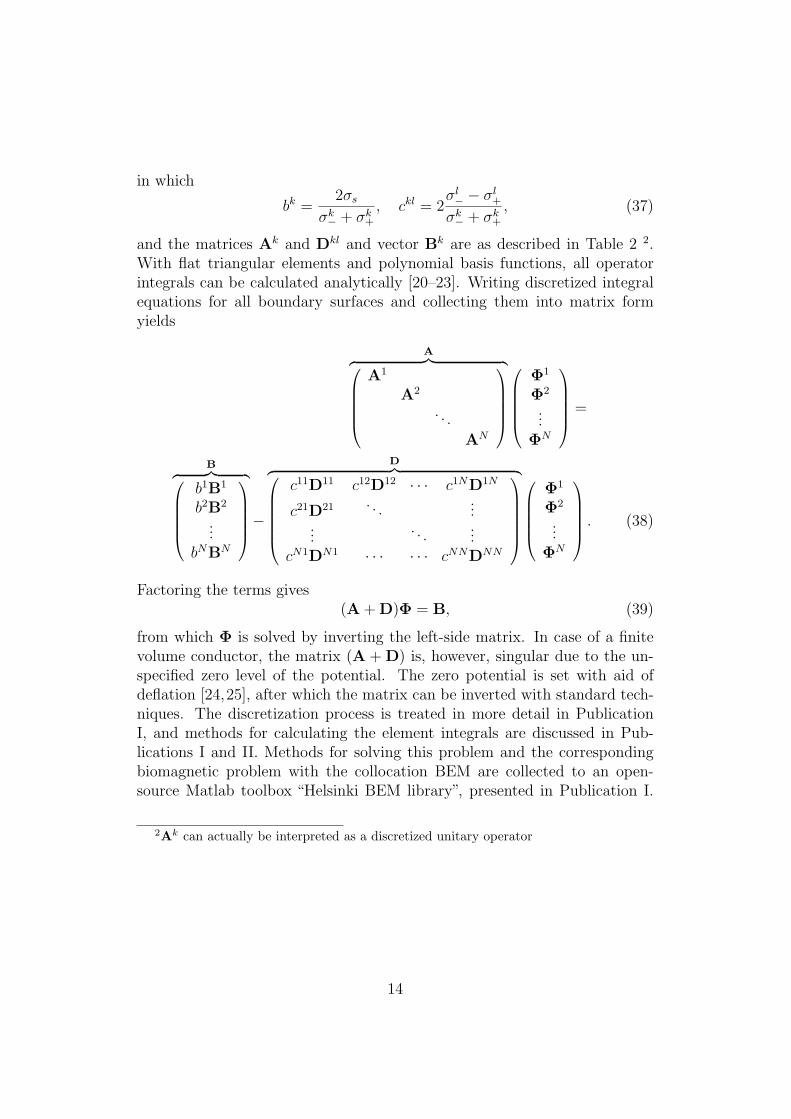
and the matrices Ak and Dkl and vector Bk are as described in Table 2 2.With flat triangular elements and polynomial basis functions, all operatorintegrals can be calculated analytically [20–23]. Writing discretized integralequations for all boundary surfaces and collecting them into matrix formyields

A︷ ︸︸ ︷⎛⎜⎜⎜⎜⎝

A1

A2

. . .

AN

⎞⎟⎟⎟⎟⎠

⎛⎜⎜⎜⎜⎝

Φ1

Φ2

...ΦN

⎞⎟⎟⎟⎟⎠ =

B︷ ︸︸ ︷⎛⎜⎜⎜⎜⎝

b1B1

b2B2

...bNBN

⎞⎟⎟⎟⎟⎠−

D︷ ︸︸ ︷⎛⎜⎜⎜⎜⎜⎝

c11D11 c12D12 · · · c1ND1N

c21D21 . . ....

.... . .

...cN1DN1 · · · · · · cNNDNN

⎞⎟⎟⎟⎟⎟⎠

⎛⎜⎜⎜⎜⎝

Φ1

Φ2

...ΦN

⎞⎟⎟⎟⎟⎠ . (38)

Factoring the terms gives(A + D)Φ = B, (39)

from which Φ is solved by inverting the left-side matrix. In case of a finitevolume conductor, the matrix (A + D) is, however, singular due to the un-specified zero level of the potential. The zero potential is set with aid ofdeflation [24,25], after which the matrix can be inverted with standard tech-niques. The discretization process is treated in more detail in PublicationI, and methods for calculating the element integrals are discussed in Pub-lications I and II. Methods for solving this problem and the correspondingbiomagnetic problem with the collocation BEM are collected to an open-source Matlab toolbox “Helsinki BEM library”, presented in Publication I.

2Ak can actually be interpreted as a discretized unitary operator

14

Table 2: Elements of the matrices resulting from discretization with constantcollocation (CC), constant Galerkin (CG), linear collocation (LC), and linearGalerkin (LG) methods. Ωl

j(�r) is the solid angle spanned by triangle j ofsurface l at �r, and �v k

i is the ith vertex of surface k. T ki labels triangle i of

surface k, Aki the area and �c k

i the centroid of that triangle.

Dklij Gkl

ij Akij Bk

i

General∫

Sk

wki D

kl[ψlj] dS

∫Sk

wki G

kl[ψlj] dS

∫Sk

wki ψ

kj dS

∫Sk

wki φ∞ dS

CC Ωlj(�c

ki ) Gkl[ψl

j](�cki ) δij φ∞(�c k

i )

LC Dkl[ψlj](�v

ki ) Gkl[ψl

j](�vki ) δij φ∞(�v k

i )

CG∫

T ki

Ωlj(�r) dS

∫T k

i

Gkl[ψlj] dS Ak

i δij

∫T k

i

φ∞ dS

LG∫

Nki

ψiDkl[ψl

j] dS∫

Nki

ψiGkl[ψl

j] dS∫

Nki

ψki ψ

kj dS

∫Nk

i

ψki φ∞ dS

2.3.3 Integral Equations for Electric Potential Outside the SourceRegion

If the sources of the electric field are not in the region of interest and thepotential or the normal derivative of the potential is known on any surfacecircumventing the source distribution, the integral equations for the electricpotential outside the source region can be stated without any source model.In electrocardiographic problems, the primary sources are in the heart muscle;the potential outside the heart can then be specified in terms of the epicardialpotential. In a homogeneous thoracic volume conductor model, this potentialproblem is formulated as an equation pair [17,26]

1

2φH = −DHB[φB] + DHH[φH] − GHH[ΓH] (40)

1

2φB = −DBB[φB] + DBH[φH] − GBH[ΓH], (41)

where ΓH = ∂φH/∂n is the normal component of the potential-gradient onthe epicardial surface, and superscripts label surfaces as presented in Fig. 1.

15

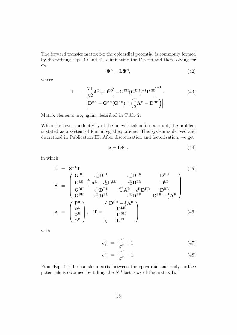
The forward transfer matrix for the epicardial potential is commonly formedby discretizing Eqs. 40 and 41, eliminating the Γ-term and then solving forΦ:

ΦB = LΦH, (42)

where

L =[(

1

2AB+DBB

)−GBH(GHH)−1DHB

]−1

· (43)[DBH + GBH(GHH)−1

(1

2AH − DHH

)].

Matrix elements are, again, described in Table 2.

When the lower conductivity of the lungs is taken into account, the problemis stated as a system of four integral equations. This system is derived anddiscretized in Publication III. After discretization and factorization, we get

g = LΦH, (44)

in which

L = S−1T, (45)

S =

⎛⎜⎜⎜⎜⎜⎝

GHH cL−DHL cR

−DHR DHB

GLH cL+2AL + cL

−DLL cR−DLR DLB

GRH cL−DRL cR+

2AR + cR

−DRR DRB

GBH cL−DBL cR

−DBR DBB + 12AB

⎞⎟⎟⎟⎟⎟⎠

g =

⎛⎜⎜⎜⎝

ΓH

ΦL

ΦR

ΦB

⎞⎟⎟⎟⎠ , T =

⎛⎜⎜⎜⎝

DHH − 12AH

DLH

DRH

DBH

⎞⎟⎟⎟⎠ (46)

with

ck+ =

σk

σB+ 1 (47)

ck− =

σk

σB− 1. (48)

From Eq. 44, the transfer matrix between the epicardial and body surfacepotentials is obtained by taking the NB last rows of the matrix L.

16

3 Forward and Inverse Problems of Electro-

cardiography

3.1 Source Modeling

In this Section, the most common source-modeling approaches used in elec-trocardiography are reviewed. The weight is on studies that either connectclosely with this study or have been applied to characterization of measuredECG datasets. Thus, e.g., computer heart models are not treated.

3.1.1 Principle

Treatment of a bioelectrical source-modeling problem is started by choosing asuitable representation for the primary current distribution �Jp. These sourcemodels aim at modeling essential properties of the underlying electrical ac-tivity while providing a feasible framework for computations. The optimalsource model depends on the specific application: for example, the earliestventricular activation of a focal arrhythmia may be localized with a point-like source model, but accurate simulation of an ischemic electrocardiogramdemands modeling of events on the cellular membrane at ion-current level.

In the boundary element formulation, the general form of a source model ispresented in Eq. 35, in which the infinite-medium potential is reconstructedby integrating the primary current density over the source volume, weightedwith the appropriate Green function. Practical applications are restricted,simplified, and optimized forms of this equation. In general, the primarycurrent density is first discretized either to a set of point-like elementarycurrent sources or to a linear combination of Ns basis functions:

�Jp(�r′) =

Ns∑j=1

Jp,j�ψj(�r

′), (49)

where �ψj(�r′) is a normalized vector-form basis function and Jp,j is the am-

plitude of the jth term of the discretized primary current distribution. Thesurface potential can then be written as a linear combination of Ns transfercoefficients Li

φ(�r) =Ns∑j=1

Jp,jLj(�r), (50)

17

where Lj(�r) is the surface potential generated by the basis function �ψj. Fora set of Nf surface points, the potential Φ can be written with help of aso-called lead-field matrix (LFM) L

Φ = LJp, (51)

where Jp contains the components Jp,j of the modeled source and Lij =Lj(�ri). With this lead-field matrix, it is straightforward and computationallyefficient to calculate the surface potential due to any modeled source (theforward problem).

Reconstruction of the modeled source from the known surface potential (theinverse problem) is done by inverting the mapping of Eq. 51. While thesolution of the forward problem is unique and, in principle, easy to compute,the inverse problem is ill-posed [27] and it does not have a unique solution [28].In order to obtain a feasible source-reconstruction, one needs to restrict thesolution space and often guide the solution to the preferred direction; thesetasks are partially carried out when choosing the source model. If the degree-of-freedom (DOF) of the source model is smaller than the DOF of the data,the source reconstruction can be performed in least-squares sense:

Jp = L†Φ, where L† = (LTL)−1LT . (52)

When the DOF of the source model is small, it may be necessary to searchfor the optimal discretization points of the source model. The relationshipbetween the positions of elementary sources and their contribution to theforward solution is non-linear. When source-positions are optimized, theproblem is typically solved in two steps: the position-search is carried outwith a non-linear optimization method, and for each test-position, the sourceamplitudes are computed with linear fitting as described above.

With distributed source models, the DOF of the source is typically largerthan the DOF of the data, leading to an under-determined problem. In sucha case, the source estimation is commonly done by means of minimum-normestimate [29] combined with some regularization method. In this Thesis, thetruncated singular value decomposition (tSVD) and Tikhonov regularizationsare used; principles of these and other regularization methods are presentedin [27].

18

3.1.2 Dipole and Multipole Models

The equivalent current dipole (ECD) is the most simple source model: thewhole primary current distribution is characterized with one current dipole�Q,

�Jp = �Qδ(�r ′), (53)

leading to the infinite-medium potential

φ∞ =1

4πσ

�Q(�r ′) · (�r − �r ′)|�r − �r ′|3 , (54)

in which �r ′ is the position of the dipole. The dipole position may be eitherfixed or time-varying (single moving dipole, SMD). With a moving dipole,the problem has three linear and three non-linear components.

In 1913, Einthoven et al. [30] characterized the mean direction of the cardiacelectric activation with a two-dimensional vector that can be reconstructedwith help of the triangle hypothesis from measurements performed with threeelectrodes. Quantitative framework for this “heart vector” and its relation tosome ECG leads was developed in [31–33]: phantom experiments with a phys-ical dipole source were performed, and the forward and inverse relationshipsbetween the three-dimensional dipolar source and four electrocardiographicleads were formulated. These results can be interpreted as the first elecrocar-diographic forward and inverse solutions, performed in terms of a pre-fixedECD. Later, the single moving dipole (SMD) model became more popular,yielding also an estimate for the location of cardiac electrical events.

The inadequacy of the dipole as a model of the cardiac electrical generatorwas realized in 1948 [33]. Non-dipolar features of the human ECG were laterdemonstrated in [34]. The clinical interpretation of the spatial properties ofthe ECG is, however, still strongly based on the concept of heart vector. TheFrank leadset [35] is the most widely-spread application for quantitative char-acterization of the heart vector; the mutually orthogonal Frank leads X, Y,and Z are reconstructed from measurements performed with seven electrodes.The transfer coefficients for these leads were defined according to phantomstudies with a physical dipole source [35].

Applications of SMD [36–45] can be divided into two partially overlappingcategories: source localization and so-called dipole ranging. In source lo-calization, limitations of the dipole source are recognized, and the methodis applied with somewhat focal sources, e.g., small infarctions [36], ectopic

19

foci [38] or accessory pathways [40]. The SMD has also been used for lo-calizing a pacing catheter [42], and the suitability of the SMD model forguiding a catheter towards the arrhythmia focus is being studied [43–45]. Indipole ranging, a dipole is fitted to the ECG at each time-instant, and dipoleparameters (moment, position) are analyzed as time–amplitude plots as inconventional ECG analysis [37,39]. The best results with the dipole rangingmethod have been obtained with focal data [36,37].

In many early SMD studies, e.g., [36, 37, 39], the volume conductor mod-eling has been performed in homogeneous thorax models using the Gabor–Nelson equations [46]. With these equations, the equivalent dipole inside ahomogeneous volume conductor can be defined via integration of the surfacepotential; inhomogeneities can not be modeled, and the potential has to beknown or interpolated over the whole surface. In [41], dipole localization wasstudied using a BEM model and a two-step dipole fitting procedure (positionsearch with non-linear optimization, moment fitted with linear least squaresmethod); this method was found preferable to the Gabor–Nelson approach.Studies [38,42] were carried out using the BEM.

In Publications IV and V, dipole models were used in detection, classification,and size-quantification of myocardial ischemia from multi-channel ECG datausing the BEM (see Section 4.3). The dipole hypothesis in these studies rosefrom dipolar patterns in body surface potential distributions; the aim wasneither to model or localize the physiological source of the cardiac electricalactivity nor to study the behavior of the heart vector in time domain. In-stead, the dipole was used as a tool for characterizing the spatial properties ofthe body surface potential distribution, for performing a physics-based geo-metrical dimension-reduction on the multi-electrode data. The applicationof the dipole in these Publications is thus more related to Einthoven’s [30]or Frank’s [35] concept of the heart-vector than to the other dipole studiesreviewed in the previous paragraphs.

The next step in the model complexity is the multipole model, in whichthe infinite-medium or boundary potential is written as a multipole seriesthat contains at least the dipole and quadrupole terms. The multipole ap-proach of source-modeling has not been used recently, perhaps due to thelack of physiological or geometrical meaning in case of the higher-order mul-tipole components. The use of a high-order multipole model can thus beinterpreted rather as dimension-reduction than as a source model. In mag-netocardiography, the second-order multipole model (dipole and quadrupole)has performed better than the dipole model in localization of a pre-excitation

20

site [47]. The use of dipole and multipole models in electrocardiography isreviewed in [48].

3.1.3 Distributed Source Models

In distributed source models, the primary current density is modeled as ei-ther a volume or a surface distribution. In volume source models, the pri-mary current density is discretized in the myocardial volume, while in surfacesource models, the sources may lie on endo- or epicardial, or on both of thesesurfaces. The directions of the elementary sources can be either free or re-stricted.

In the review [48], “multiple dipole models” are treated. In some of thesemodels, each dipole represents the mean electrical activity of a specific car-diac region; such an approach can as well be interpreted as discretizationof the primary current distribution. Thus, [48] serves also as a review onearly studies on distributed source models. A volume source model has laterbeen used for, e.g., estimation of the viable myocardium from electro- andmagnetocardiographic data [49]. In one example in Publication I, a surfacesource model spanned at the endo- and epicardium is used for localization ofa region of simulated myocardial ischemia.

The equivalent double-layer model (EDL) [50–53] is an application of thesurface source model, in which a simple model of cardiac depolarization isutilized: A depolarization wavefront is modeled as a uniform double-layer(UDL). As long as this layer is closed, it produces no external potential.When the wavefront reaches either the endo- or epicardium, the double-layeropens up, contributing to the electrocardiogram. The open double-layer canbe modeled as a sum of a closed layer and an oppositely-directed open UDLat the region of the opening. Thus, the source of the external potential canbe modeled as an equivalent double-layer spanned at endo- and epicardialsurfaces. The infinite-medium potential due to the EDL can then simply bestated in terms of the double-layer operator,

φ∞ =1

σs

DH[sH], (55)

where H is the union of endo- and epicardial surfaces and sH is the EDLstrength (the normal component of the primary current). The tools that areused in Section 2.3.2 apply also to discretization of the EDL source.

21

The bidomain theory of the cardiac muscle [51, 54] provides the theoreti-cal framework for the double-layer source model: In the bidomain theory,the cardiac muscle is modeled as a continuum of intertwined intra- and ex-tracellular spaces that are connected via currents passing through the cellmembrane. With help of this theory, the relationship between the primarycurrent �Jp and the transmembrane potential (TMP) φm can be written [54]

�Jp = −σi∇φm, (56)

where σi is the intracellular conductivity. In a homogeneous compartment ofcardiac tissue, the infinite-medium potential generated by the volume TMPcan be written directly in terms of the surface TMP [51,52]:

φ∞ = −σi

σs

DH[φm]. (57)

The connection between the surface TMP and the extracellular potentialenables the use of knowledge on cardiac action potential. This feature isutilized effectively in applications of the EDL. The EDL method has, inaddition to depolarization, also been applied to the repolarization [52]. Inthe ECGSIM program3 [53], simulation of the electrocardiogram is based onendo- and epicardial action potential waveforms that can be altered in timeand shape. The volume conductor modeling in [50,52,53] is performed withthe boundary element method, applying the point collocation weighting andtaking into account the effects of lungs and intracardiac bloodmasses.

In activation time imaging (ATI) and its application “Noninvasive Imagingof Cardiac Electrophysiology” (NICE) [55], the TMP model is utilized in in-verse reconstruction of cardiac activation times. In simulation study [25],pre-defined action potential waveform and a time-course model of the ven-tricular depolarization were coupled with both point collocation and GalerkinBEMs; the Galerkin method performed better in the forward computationdue to the more accurate reproduction of the depolarization-time informa-tion. This benefit did, however, not reflect to results of [56], in which ATI wasperformed on a patient with Wolff–Parkinson–White (WPW) syndrome us-ing both collocation and Galerkin BEMs and the FEM; all methods producedvery similar activation time maps. The ATI method has been successfullyapplied to localization of a WPW accessory pathway [55–57] and of a sur-face breakthrough of paced data in the right atrium [58] and in the rightventricle [56]. Activation time maps obtained from healthy volunteers havebeen morphologically similar to those obtained earlier from isolated humanhearts [57].

3ECGSIM was used in Publication I for simulating the ischemic electrocardiogram.

22

3.2 Epicardial Potential Imaging

In epicardial potential imaging [17, 26, 59–61], the electric potential on thesurface of the heart outside the myocardium is reconstructed from electro-cardiographic data. Formulating the cardiac inverse problem in terms ofepicardial potential instead of using source models has four kinds of advan-tages [62]:

1. The solution is unique: if the potential is known over any closed surfacecomprising all sources, potential anywhere outside the source region isuniquely defined.

2. No restrictive assumptions regarding the nature and complexity ofsources are made.

3. Intracardiac blood masses and cardiac anisotropy are taken into ac-count implicitly—they do not need to be modeled.

4. Inverse solutions can be validated by comparing them to invasivelymeasured epicardial electrograms.

Although the epicardial potential problem has a unique solution, the problemis ill-posed, and the inverse problem needs to be solved with help of similarregularization methods that are used in source-modeling problems [27].

3.2.1 Computational Methods in Epicardial Potential Imaging

The epicardial potential problem was for the first time formulated for arealistically-shaped geometry in [26] using a collocation BEM approach, inwhich the potential was approximated with constant basis functions, but thecollocation points were placed in the nodes instead of the triangle centroidsof the mesh. Other early methods and applications are reviewed in [62], inwhich simulations with an eccentric-spheres model are presented as well.

Linear collocation BEM has been applied to the epicardial potential problemin, e.g., [17,63] and almost all studies of the Rudy research group [64]. In [17],performances of the constant and linear collocation methods were comparedusing simulated data; the constant method was found more accurate. Theseresults are discussed in more detail in Publication II, in which the same Dal-housie thorax model as in [17] was used. Second-order basis functions haverecently been applied with the collocation method, leading to encouraging

23

results [64]: With a canine heart and a thorax-shaped saline tank, the re-construction error of the electrograms over the cardiac cycle decreased byapproximately 20 percentage units compared to the linear basis. In a pacedhuman heart, the quadratic method localized the pacing site more accuratelythan the linear method did. In addition to the BEM, also the finite elementmethod (FEM) [65] and a combined FEM–BEM approach [66] have beensuggested. These methods have not gained popularity yet, but they enablethe important possibility to model anisotropic structures. Thus far such in-formation is not routinely available, but this may change in the near futuredue to the development of diffusion-tensor magnetic resonance imaging.

In Publication II, the Galerkin BEM was applied to the epicardial potentialproblem for the first time. In computation of the single-layer element inte-grals, analytical formulas [22] were used for the first time, eliminating oneoften-discussed source of uncertainty. The linear Galerkin (LG) method gavesmaller discretization errors on the epicardium and forward transfer errorson the body surface than the other tested methods did. These results did,however, not reflect to the Tikhonov-regularized inverse problems, unless theerror was evaluated as integral over the whole epicardial surface. Overall, thechoice of basis and weight functions had smaller effect on the reconstructedepicardial potential than the errors due to interpolation and insufficient mod-eling did.

In choosing the basis functions for boundary element computations, the er-ror introduced by interpolation of the source data should not be overlooked.Constant basis and weight functions are spanned according to the triangles,while their linear counterparts are built around the nodes of the mesh. Theresults of computations are thus written in terms of triangle and node poten-tials, respectively. In the meshing process, nodes are commonly placed intoelectrode positions. If constant basis functions are used with such a mesh, thedata measured with the electrodes need to be interpolated from the electrodepositions to the triangles. In Publication II, the effect of such interpolationon inverse problem was studied: In optimal modeling conditions with simu-lated data, the interpolation increased the reconstruction error considerably.In realistic applications, however, the error due to the interpolation is prob-ably not as large as in the optimal model, because smoothing caused by theinterpolation appears to partially compensate for the modeling errors (seeFigs. 4 and 5 and Section V-E in Publication II). Still, if computations canbe done directly using the data at electrode positions only, there is no reasonfor interpolating the measured data before solving the inverse problem.

24

Recently, the method of fundamental solutions (MFS) was applied to theepicardial potential problem [67]. The use of MFS was motivated by listingproblems of the BEM: singular integrals, difficulty of implementation, andmesh-related artifacts. For all these problems, there is, however, a solution ora work-around: The singular integral of the G operator can, with flat trian-gles and polynomial basis functions, be calculated analytically [22, 23]. Theother singularity-related problem, the “auto-solid angle” in the discretizationof the D operator [68], is not an issue in the constant methods or in the linearGalerkin method, in which the actual field computation points are inside ofsmooth triangles instead of being in the sharp nodes (see Publication II).Compact, general presentation of the mathematics of the epicardial poten-tial problem (Publications II and III) and the thorough documentation ofthe analytical integrals in [22] coupled with the BEM library presented inPublication I enable the straightforward implementation of the BEM solver.The use of the linear Galerkin method reduces mesh-related artifacts, be-cause computations do not need to be performed at sharp-angled nodes ofthe mesh.

3.2.2 Volume Conductor Modeling in Epicardial Potential Imag-ing

The first BEM implementation of the epicardial potential problem [26] wasformulated in a homogeneous volume conductor. A formulation for a piece-wise homogeneous volume conductor was reported in [69], but it has appar-ently not been applied to epicardial potential imaging later on. Difficultiesand limitations of [69] are discussed in Publication III, in which a generalized,operator-based formulation of the problem is presented and validated. Effectsof conductivity inhomogeneities on the forward epicardial potential problemhave—in realistically shaped models—been studied, e.g., in [69–71] and inPublication II. In the inverse epicardial potential problem, these effects havebeen studied in [72,73] and in Publication II.

In [69], epicardial and body surface potential data were measured from anintact dog. Boundary element models with various simplifications were con-structed, and computed surface potentials were compared to the measuredones, using the measured epicardial potentials as input data. Anisotropic tho-racic muscle was approximated as suggested in [74], replacing the anisotropiclayer with a scaled isotropic layer. The full model comprised the lungs, ster-num, spine, and thoracic muscle layer. During sinus rhythm, this model leadto relative error (RE) of 39%. The muscle layer was found to be the most

25

important inhomogeneity: removing it increased the RE to 56%, while re-moving of all inhomogeneities gave the RE of 58%. With anterior pacing,errors were considerably larger. The effect of lungs was found insignificant.It is, however, not clear, how well these results are applicable to the humanthorax; especially the structure and size of the muscle layer and the validityof the used approximation may differ.

An accurate FEM thorax model containing the lungs, anisotropic musclelayer, various fat pads, and major bones and blood vessels was built in [70].Body surface potential maps were computed in the model containing all in-homogeneities, using a measured epicardial potential distribution. Thesebody surface maps were then compared to corresponding maps obtainedwith simplified models using the same epicardial potential distribution. Theanisotropic thorax muscle, subcutaneous fat, and lungs played the largestroles, causing 12–15% relative errors each.

In [71], a perfused canine heart and a homogeneous torso-shaped saline tankwere used. The heart was paced from various positions, and epicardial andsurface potentials were measured. The solution of the forward problem inthe homogeneous volume conductor was first validated against the measureddata. Then, the model geometry was altered and inhomogeneities were intro-duced computationally, and the effects of inhomogeneities on the tank surfacepotential were compared against each other. The relative difference4 betweenthe computed surface potentials in homogeneous and inhomogeneous modelswas between 7% and 17%. The conclusion was that inhomogeneities haveonly minor effects on the electrocardiogram.

In [70,71], the epicardial potential was assumed fixed, and differences betweencomputed surface solutions were evaluated. Thus, the effect of the volumeconductor variation on the epicardial potential was omitted. This causeserrors regarding the roles of the inhomogeneities, especially those close tothe heart. Overall, the role of the inhomogeneities can not be fully assessedby studying the forward problem only, because in the inverse problem, smallerrors in the computational model or measured data may lead to large errorsin the inverse reconstruction [27].

In [72], the EDL model was used for simulation of realistic epicardial5 and

4Relative difference is mathematically identical to the relative error, presented in Eq.29 of Publication II

5In [72] and other studies of the van Oosterom group, the term “pericardial potential”is used instead of “epicardial potential”.

26

body surface potentials in a piece-wise homogeneous volume conductor (in-tracardiac blood masses, lungs). Then, epicardial potentials were recon-structed utilizing a priori information of the solution. Evaluation of differentvolume conductor simplifications was not elaborated, but it was concludedthat, in order to obtain proper results, the lungs need to be included.

The study [71] was followed by [73], in which the same measured epicardialpotential patterns were used for computational generation of body surfacepotential maps in a piece-wise homogeneous model. Then, the inverse po-tential problem was solved using various model simplifications. The relativeerror increased by about 20 and the correlation coefficient decreased by lessthan 10 percentage units, when the inhomogeneities were left out. It wasthen concluded that modeling of the inhomogeneities can be omitted.

In Publication II, both forward and inverse problem were first solved in a ho-mogeneous model. Then, inhomogeneities were introduced in the generationof the reference data, while the inverse reconstruction was performed usingthe homogeneous model. In the optimal modeling conditions (both forwardand inverse transfers in identical, homogeneous models), the median relativeerror of the inverse reconstruction was approximately 10%. When the for-ward problem was solved in a model containing the lungs and the inversereconstruction was done in a homogeneous model, the corresponding errorwas about 30%.

In [71,73], it was discussed that the inclusion of the inhomogeneities increasesthe condition number of the forward transfer matrix, leading to a more ill-posed inverse problem and thus devaluing the advantage of the more accuratetransfer matrix. In Publication III, however, the condition number of the for-ward transfer matrix for the inhomogeneous model was smaller than that forthe corresponding homogeneous model. In other words, modeling of inho-mogeneities with the method described in Publication III does not increasethe ill-posedness of the problem. The use of a piece-wise homogeneous tho-rax model instead of the homogeneous one thus prepares the way for moreaccurate reconstruction of epicardial potential.

3.2.3 Validation of Epicardial Potential Imaging

Major part of method development in epicardial potential imaging is based ondata measured with a semi-realistic phantom: a Langendorff-perfused canineheart placed into a thorax-shaped saline tank that is equipped with surface

27

electrodes and electrode rods (see [59]). With this setup, voltages both onthe surface of the tank and close to the epicardium can be recorded syn-chronously. Such data are ideal for developing and comparing computationalmethods, but the role of the inhomogeneous volume conductor and errors dueto simplifications in the volume conductor model can not be directly studied.Tank studies and other validation approaches to both epicardial potentialimaging and source-modeling have been reviewed, e.g., in [75,76].

Epicardial potential imaging is currently being validated with realistic hu-man data. So far, epicardial potential imaging has been shown to localizeventricular pacing sites with accuracy of about 10 mm [64]. In comparisonto electrograms measured invasively from the epicardial surface, epicardialpotential imaging has been able to characterize essential features of depolar-ization: results in [61] suggest that earliest ventricular activation and areasof slow conduction can be localized, and that the general excitation patterncan be captured. In the same study, reconstructed electrograms were in mod-erately good morphological concordance with measured signals (correlationcoefficient ≈ 0.7); amplitude errors were not reported. Total excitation pat-terns computed from epicardial potential maps have been similar to thosemeasured earlier from isolated hearts [60].

The validation results discussed above have been obtained with homogeneousvolume conductor models; inclusion of the lungs in the computational modelwill improve the results further.

28

4 Detection and Localization of Myocardial

Ischemia

4.1 Myocardial Ischemia and the Electrocardiogram

Coronary artery disease leads to occlusion of coronary arteries. The occlusioncauses reduction of blood supply in myocardium. The reduced blood-flowleads to disturbed hemodynamics and lack of oxygen that cause changes inelectrophysiological conditions of the cardiac muscle cells. These changes al-ter the transmembrane potential in the ischemic region, leading thus to ECGchanges. Prolonged ischemia leads to myocardial infarction, in which per-manent damage for cardiac muscle cells has occurred. Myocardial infarctionincreases the risk of possibly lethal ventricular arrhythmias and weakens thepumping-function of the heart. [77]

Ischemic changes in the electrocardiogram are typically easiest to detect be-tween depolarization and repolarization of the ventricular myocardium. InECG waveforms, this plateau phase is referred to as ST segment; labelingof the ECG waveform is presented in Fig. 3. During the plateau phase,the transmembrane potential is larger in healthy myocardium than in theischemic region. This potential-difference generates changes in the epicar-dial potential and electrocardiogram: Transmural ischemia causes epicardialand electrocardiographic ST potential elevation in the region overlying theischemic area, while subendocardial ischemia may cause either ST elevation,depression, or no ST change at all [78–82]. Overall, the strength and shapeof ischemic ST changes depend on the extent and severity of the ischemia, onintra- and extracellular conductivities, and on the direction of cardiac musclefibers [78–81,83]. The current flow and changes of epicardial potential asso-ciated with subendocardial ischemia have been characterized and visualizedin [79,80].

In addition to the ST segment, myocardial ischemia may alter also otherfeatures of the electrocardiogram, especially the QRS complex and T wave;a recent listing of electrocardiographic abnormalities that may evolve to my-ocardial infarction is provided in [84]. In addition, ECG markers such asQRS slope [85] and high-frequency content of the QRS complex [86] havebeen reported to add to the value of the ECG in diagnosis of myocardialischemia. It has also been reported [87–89] that electrodes outside the stan-dard 12-lead setup improve the electrocardiographic detection of myocardial

29

ischemia. In [87, 88], the optimal unipolar [88] or bipolar leads [87] for de-tecting ischemia were derived by searching for the largest [87] or statisticallymost significant [88] alterations in ST60 (see Fig. 3) body surface potentialmaps measured during induced ischemia. The electrode layouts suggestedin [87,88] were applied in Publication IV.

In Publications IV–VI, both ST potentials and other linear ECG markersare used in detection, localization, and size quantification of myocardial is-chemia, applying dipole modeling and epicardial potential imaging. To theauthor’s knowledge, dipole modeling has not been used before in quantita-tive analysis of the myocardial ischemia. In Dalhousie university, the ischemicelectrocardiogram has been studied using a measurement system and datasetvery similar to ours; epicardial potential imaging has been applied to char-acterization of ischemia in, e.g., [63,90].

4.2 Datasets and Preprocessing

The datasets used in Publications IV–VI were collected in Division of Cardiol-ogy at Helsinki University Central Hospital. Body surface potential mappingwas performed using BioSemi Mark VI and Active Two amplifiers6 and stripelectrodes. The measurement system is described in [91], and the electrodelayout is visualized in Fig. 4a of this text and in Fig. 1 of Publication IV.

In percutaneous transluminal coronary angioplasty (PTCA), a catheter withan inflatable balloon is inserted into the occluded coronary artery, and theartery is re-opened by inflating the balloon at the occlusion site [92]. Dur-ing the inflation, the artery is totally blocked, leading to temporary supplyischemia. PTCA provides an idealized model of the ischemic myocardium:the site of the occlusion is known, and the artery is totally blocked.

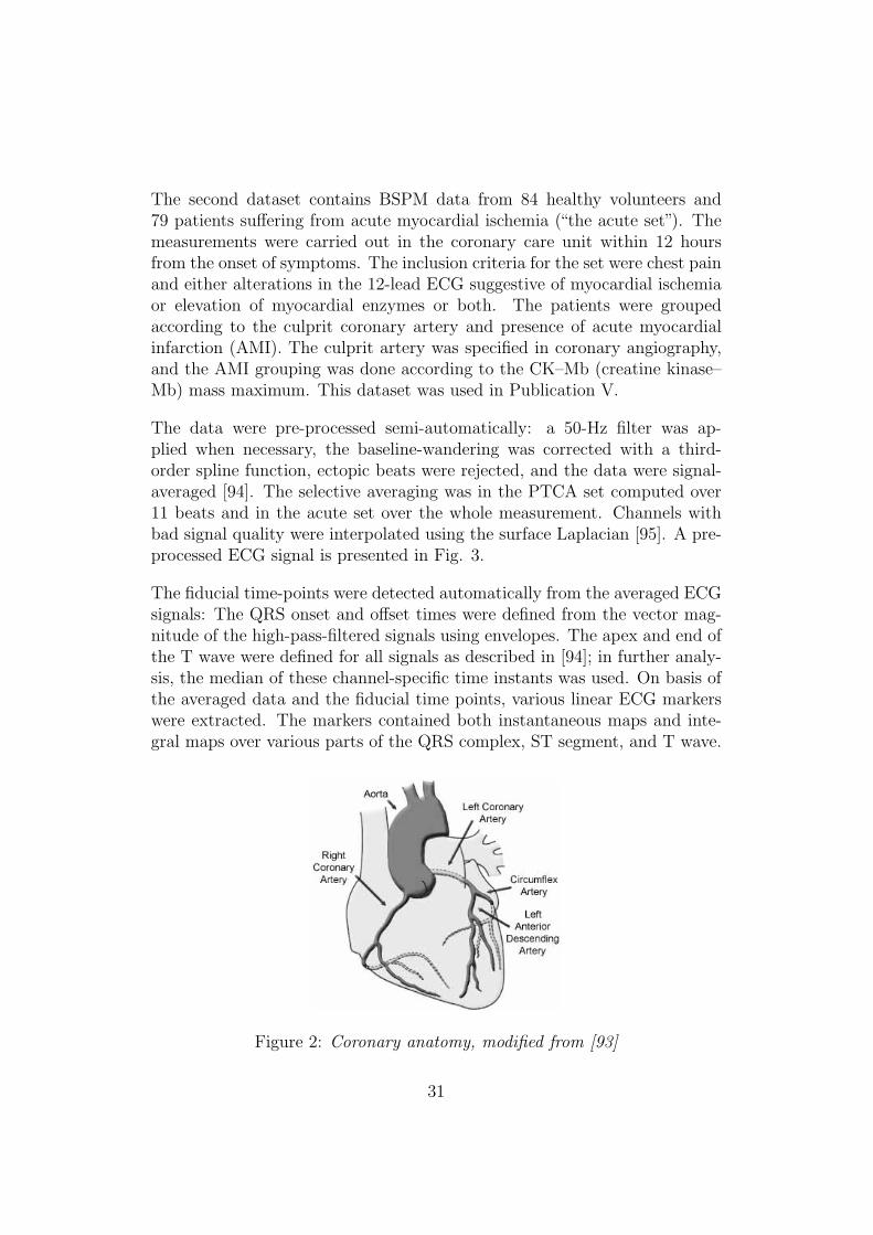
In the first dataset (“the PTCA set”), the BSPM was measured in the catheterlaboratory during scheduled PTCA operations in 22 patients. The angio-plasty was performed in left anterior descending (LAD, n = 8), left cir-cumflex (LCX, n = 7), or right coronary artery (RCA, n = 7). Typicalcoronary artery anatomy is visualized in Fig. 2. This dataset was used inPublications IV and VI. BSPM data measured during PTCA were also usedin [63, 87, 88, 90]; the electrode layout was nearly identical to that in ourstudies.

6http://www.biosemi.com

30

The second dataset contains BSPM data from 84 healthy volunteers and79 patients suffering from acute myocardial ischemia (“the acute set”). Themeasurements were carried out in the coronary care unit within 12 hoursfrom the onset of symptoms. The inclusion criteria for the set were chest painand either alterations in the 12-lead ECG suggestive of myocardial ischemiaor elevation of myocardial enzymes or both. The patients were groupedaccording to the culprit coronary artery and presence of acute myocardialinfarction (AMI). The culprit artery was specified in coronary angiography,and the AMI grouping was done according to the CK–Mb (creatine kinase–Mb) mass maximum. This dataset was used in Publication V.

The data were pre-processed semi-automatically: a 50-Hz filter was ap-plied when necessary, the baseline-wandering was corrected with a third-order spline function, ectopic beats were rejected, and the data were signal-averaged [94]. The selective averaging was in the PTCA set computed over11 beats and in the acute set over the whole measurement. Channels withbad signal quality were interpolated using the surface Laplacian [95]. A pre-processed ECG signal is presented in Fig. 3.

The fiducial time-points were detected automatically from the averaged ECGsignals: The QRS onset and offset times were defined from the vector mag-nitude of the high-pass-filtered signals using envelopes. The apex and end ofthe T wave were defined for all signals as described in [94]; in further analy-sis, the median of these channel-specific time instants was used. On basis ofthe averaged data and the fiducial time points, various linear ECG markerswere extracted. The markers contained both instantaneous maps and inte-gral maps over various parts of the QRS complex, ST segment, and T wave.

Figure 2: Coronary anatomy, modified from [93]

31

Am

plitu

de/m

V

Time / ms

QRSonset

QRSoffset

T apex

T endST60

QRS 1 / 4 integral QRS 2 / 4 integral ST integral

-200 -100 0 100 200 300 400

-0.4

-0.2

0

0.2

0.4

0.6

QRST integral

Figure 3: A preprocessed ECG signal with fiducial time-points, ST60 time-instant, and various integral markers. The QRS complex is the period betweenthe QRS onset and offset, and the ST segment starts from the QRS offsetand continues as the T wave. The T wave onset-point was not defined orused in this study.

The fiducial time points and some of these markers are illustrated in Fig. 3.For the PTCA set, delta maps [87] were generated by subtracting the mapbefore the balloon inflation from the map with maximal ST changes. Thedelta maps thus represent only the ECG alterations caused by the balloon.

4.3 Dipole Modeling

In Publications IV and V, dipole modeling is applied in spatial characteriza-tion of measured electrocardiograms. While both studies deal with ischemichearts, aims and methods are different: In Publication IV, the aim is toclassify the ischemic electrocardiogram according to the coronary artery ex-periencing reduced flow, and the classification is based on angles betweendipoles. In Publication V, it is studied, whether simple parameters derivedfrom dipoles are able to discriminate patients from controls and predict theextent of the resulting infarction as measured by creatine kinase–Mb enzyme.

32

These discriminating or predicting parameters include, e.g., amplitudes of or-thogonal components or projections of the dipole.

The dipole hypothesis in these studies originated from dipolar patterns ob-served in body surface potential maps (see Fig. 2 in Publication IV). Theaim was not to localize the source of the abnormal cardiac electrical activitywith help of the dipolar source model. Instead, the dipole was used as a toolfor characterizing the morphology of the body surface potential distribution(see also Section 3.1.2).

4.3.1 PTCA Set (Publication IV)

In the PTCA delta maps presented in [87], the population-average mapsof the ST60 potential7 show dipolar morphology, and the map orientationdepends on the occluded artery. In our PTCA set, the corresponding mapswere very similar to those in [87]. In Publication IV it was studied, whetherthe map orientation can be characterized with a dipole model, and whetherthe resulting dipoles can be used for discriminating between culprit arteries.The ST60 population-average maps and corresponding dipoles of our PTCAset are visualized in Figs. 2 and 3 of Publication IV.

Computation of the equivalent current dipoles was performed as described inPublications IV and V using the development version of the BEM library pre-sented in Publication I. The dipole position was either optimized for the bestreconstruction of the measured data in each patient (“best-reconstructing”),pre-fixed, or defined from the population average maps (“artery-specific”).

In all patients, the Dalhousie thorax model [17] was used; variation in patientanatomy and electrode positioning was omitted. The thorax model was as-sumed otherwise homogeneous, but the anisotropic thoracic muscle layer wasapproximated as suggested in [1, 74], replacing the anisotropic layer with ascaled isotropic layer. When this volume expansion method was applied, thedipoles fitted to the dataset had, according to visual inspection, smaller vari-ation than in the fully homogeneous model. In the first classification tests,the volume-expanded model also performed better than the homogeneousone. All further analysis was thus done with the expanded model.

In addition to the full BSPM set, five reduced electrode-sets were applied:those of the 12- and 18-lead [89] ECGs, a custom set modified from the 12-

7ST60 potential = potential 60 ms after the QRS offset

33

a b

c d

e f

Figure 4: Electrode setups used for ischemia classification. a) BSPM, b) 12-lead, c) modified 12-lead, d) 18-lead [89], e) Horacek [87], and f) Kornreich[88].

lead set (“modified 12-lead”), and the 5-electrode sets proposed in [87, 88].Although the datasets and principles of discrimination in [87,88] were similarto those used in this Thesis, there is an essential difference: in [87, 88], thebest electrode positions for a given ECG marker were sought for, whereasin the dipole studies of this Thesis, the main spatial features of potentialdistribution sampled by a given electrode-set are distilled into one dipole,which is then used for classification.

The electrode layouts of the applied electrode-sets are visualized in Fig. 4.The reduced-set data were generated from the BSPM markers; to enable fieldcalculation in the 12- and 18-lead sets, the limb electrodes were positionedon shoulders and left hip and the chest electrodes were placed in the best-matching nodes of the thorax model. ECG markers at positions that didnot match with the electrodes of the BSPM set were interpolated using thesurface Laplacian [95].

Patients were classified by comparing the dipole moment computed fromthe test case (“test dipole”) to the corresponding dipole moments computed

34

from the population average maps of other patients in leave-one-out manner:the test dipole was always independent on the data used for obtaining thepopulation average maps. The cosine of the angle between the dipoles waschosen as the classification parameter. When reduced electrode-sets wereused, the population average maps were constructed with both BSPM andthe set in question. After preliminary testing, only the ST60 potential wasused in classification.

With the BSPM set, 21 of the 22 patients were classified correctly using anydipole positioning. When reduced sets were used, the pre-fixed or artery-specific dipole positions performed better than the best-reconstructing dipoledid. The modified 12-lead set performed as well as the BSPM, and the 5-electrode set of [87] was able to classify 20 patients correctly. The 12-lead setprovided the correct classification in 18 cases, while the 18-lead set succeededin either 19 or 20 cases. The 5-electrode system suggested in [88] seems tobe badly suitable for use with dipole modeling. With reduced electrode-setsand artery-specific dipoles, the positions defined according to the BSPM dataperformed better than those defined with the set being tested.

These results show that dipole modeling is a powerful tool for characterizingthe orientation of body surface potential maps. The method presented hereis applicable also with reduced electrode-sets, especially when the dipolepositions are pre-fixed according to prior BSPM results. In addition to thequantitative information obtained from the dipoles, the use of the dipolemodel provides a way for visualizing the heart vector, thus facilitating themanual interpretation of the electrocardiogram.

4.3.2 Acute Set (Publication V)

In Publication V, dipole modeling was used for detection of myocardial is-chemia and size quantification of the resulting myocardial infarction. Thedataset was subdivided according to the culprit coronary artery and presenceof myocardial infarction, resulting in eight patient categories (see Table 2 inPublication V). The field computation was done with the same model asin Publication IV, and the dipole position was either the pre-fixed or best-reconstructing one.

First, dipoles were fitted to all BPSM markers resulting from the preprocess-ing, using either the full BSPM set or the electrode set of the reconstructed12-lead ECG. Next, 10 parameters were extracted from each dipole. Then,

35

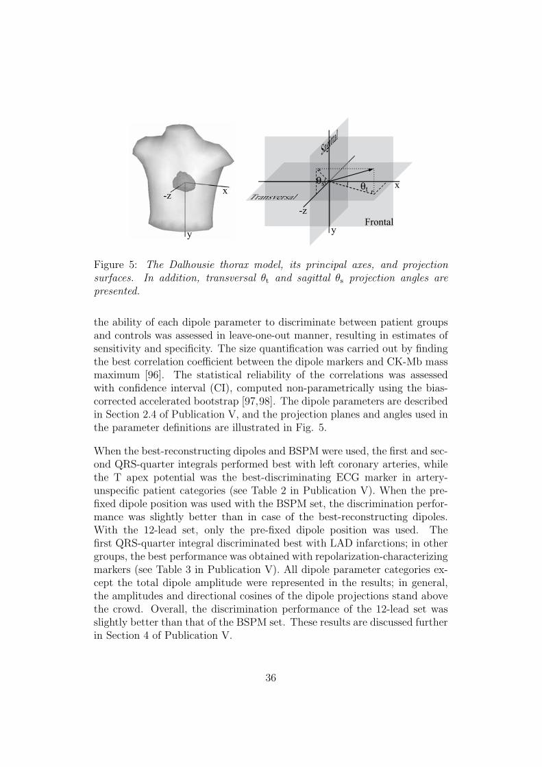
x

y

-z TransversalTrTT anansversalθt

θs

y

-zFrontal

x

Sagittal

Figure 5: The Dalhousie thorax model, its principal axes, and projectionsurfaces. In addition, transversal θt and sagittal θs projection angles arepresented.

the ability of each dipole parameter to discriminate between patient groupsand controls was assessed in leave-one-out manner, resulting in estimates ofsensitivity and specificity. The size quantification was carried out by findingthe best correlation coefficient between the dipole markers and CK-Mb massmaximum [96]. The statistical reliability of the correlations was assessedwith confidence interval (CI), computed non-parametrically using the bias-corrected accelerated bootstrap [97,98]. The dipole parameters are describedin Section 2.4 of Publication V, and the projection planes and angles used inthe parameter definitions are illustrated in Fig. 5.

When the best-reconstructing dipoles and BSPM were used, the first and sec-ond QRS-quarter integrals performed best with left coronary arteries, whilethe T apex potential was the best-discriminating ECG marker in artery-unspecific patient categories (see Table 2 in Publication V). When the pre-fixed dipole position was used with the BSPM set, the discrimination perfor-mance was slightly better than in case of the best-reconstructing dipoles.With the 12-lead set, only the pre-fixed dipole position was used. Thefirst QRS-quarter integral discriminated best with LAD infarctions; in othergroups, the best performance was obtained with repolarization-characterizingmarkers (see Table 3 in Publication V). All dipole parameter categories ex-cept the total dipole amplitude were represented in the results; in general,the amplitudes and directional cosines of the dipole projections stand abovethe crowd. Overall, the discrimination performance of the 12-lead set wasslightly better than that of the BSPM set. These results are discussed furtherin Section 4 of Publication V.

36

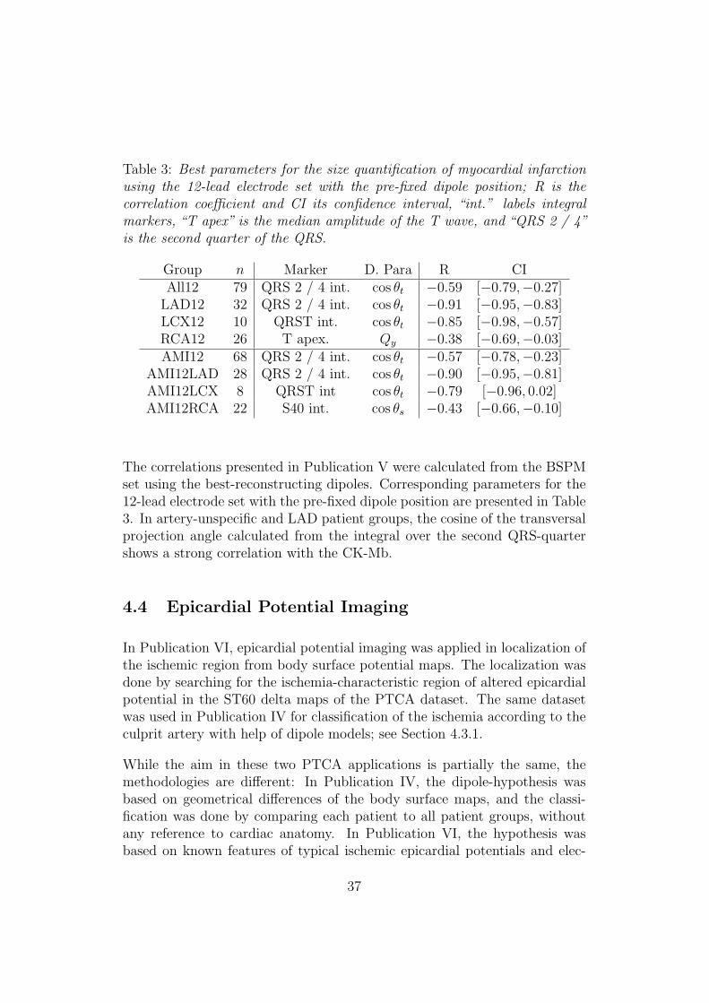
Table 3: Best parameters for the size quantification of myocardial infarctionusing the 12-lead electrode set with the pre-fixed dipole position; R is thecorrelation coefficient and CI its confidence interval, “int.” labels integralmarkers, “T apex” is the median amplitude of the T wave, and “QRS 2 / 4”is the second quarter of the QRS.

Group n Marker D. Para R CIAll12 79 QRS 2 / 4 int. cos θt −0.59 [−0.79,−0.27]

LAD12 32 QRS 2 / 4 int. cos θt −0.91 [−0.95,−0.83]LCX12 10 QRST int. cos θt −0.85 [−0.98,−0.57]RCA12 26 T apex. Qy −0.38 [−0.69,−0.03]AMI12 68 QRS 2 / 4 int. cos θt −0.57 [−0.78,−0.23]

AMI12LAD 28 QRS 2 / 4 int. cos θt −0.90 [−0.95,−0.81]AMI12LCX 8 QRST int cos θt −0.79 [−0.96, 0.02]AMI12RCA 22 S40 int. cos θs −0.43 [−0.66,−0.10]

The correlations presented in Publication V were calculated from the BSPMset using the best-reconstructing dipoles. Corresponding parameters for the12-lead electrode set with the pre-fixed dipole position are presented in Table3. In artery-unspecific and LAD patient groups, the cosine of the transversalprojection angle calculated from the integral over the second QRS-quartershows a strong correlation with the CK-Mb.

4.4 Epicardial Potential Imaging

In Publication VI, epicardial potential imaging was applied in localization ofthe ischemic region from body surface potential maps. The localization wasdone by searching for the ischemia-characteristic region of altered epicardialpotential in the ST60 delta maps of the PTCA dataset. The same datasetwas used in Publication IV for classification of the ischemia according to theculprit artery with help of dipole models; see Section 4.3.1.

While the aim in these two PTCA applications is partially the same, themethodologies are different: In Publication IV, the dipole-hypothesis wasbased on geometrical differences of the body surface maps, and the classi-fication was done by comparing each patient to all patient groups, withoutany reference to cardiac anatomy. In Publication VI, the hypothesis wasbased on known features of typical ischemic epicardial potentials and elec-

37

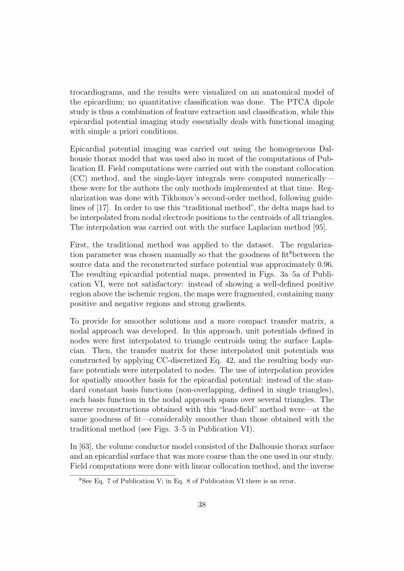
trocardiograms, and the results were visualized on an anatomical model ofthe epicardium; no quantitative classification was done. The PTCA dipolestudy is thus a combination of feature extraction and classification, while thisepicardial potential imaging study essentially deals with functional imagingwith simple a priori conditions.

Epicardial potential imaging was carried out using the homogeneous Dal-housie thorax model that was used also in most of the computations of Pub-lication II. Field computations were carried out with the constant collocation(CC) method, and the single-layer integrals were computed numerically—these were for the authors the only methods implemented at that time. Reg-ularization was done with Tikhonov’s second-order method, following guide-lines of [17]. In order to use this “traditional method”, the delta maps had tobe interpolated from nodal electrode positions to the centroids of all triangles.The interpolation was carried out with the surface Laplacian method [95].

First, the traditional method was applied to the dataset. The regulariza-tion parameter was chosen manually so that the goodness of fit8between thesource data and the reconstructed surface potential was approximately 0.96.The resulting epicardial potential maps, presented in Figs. 3a–5a of Publi-cation VI, were not satisfactory: instead of showing a well-defined positiveregion above the ischemic region, the maps were fragmented, containing manypositive and negative regions and strong gradients.

To provide for smoother solutions and a more compact transfer matrix, anodal approach was developed. In this approach, unit potentials defined innodes were first interpolated to triangle centroids using the surface Lapla-cian. Then, the transfer matrix for these interpolated unit potentials wasconstructed by applying CC-discretized Eq. 42, and the resulting body sur-face potentials were interpolated to nodes. The use of interpolation providesfor spatially smoother basis for the epicardial potential: instead of the stan-dard constant basis functions (non-overlapping, defined in single triangles),each basis function in the nodal approach spans over several triangles. Theinverse reconstructions obtained with this “lead-field” method were—at thesame goodness of fit—considerably smoother than those obtained with thetraditional method (see Figs. 3–5 in Publication VI).

In [63], the volume conductor model consisted of the Dalhousie thorax surfaceand an epicardial surface that was more coarse than the one used in our study.Field computations were done with linear collocation method, and the inverse

8See Eq. 7 of Publication V; in Eq. 8 of Publication VI there is an error.

38

transfer matrix was constructed with help of the Tikhonov regularization, inwhich the regularization parameter was set with help of simulated data. Theanalysis was carried out using delta maps constructed from ST integral maps.Results were, according to visual comparison, slightly more detailed thanthose obtained with the lead-field method in our study, but much smootherthan those resulting from the traditional method.

While the lead-field method and the method applied in [63] are able to yieldsmooth epicardial potential maps that reflect geometrical features of the bodysurface potential maps, they may, due to modeling errors or under- or over-regularization, fail in giving a clear estimate on the location and extent ofthe ischemic region. In order to provide for an easy-to-interpret, robust toolfor localization of the ischemic region, another method was developed. Inthis “template method”, the epicardial potential around each node of the epi-cardial mesh is modeled with help of a pre-specified neighborhood function.From these template epicardial potential maps, corresponding body surfacepotential maps are computed and used for iterative searching of the templatethat best fits the measured data.

Results obtained with the template method are, for representative cases, dis-played in Figs. 3c–5c and Fig. 6 of Publication VI. The template methodproduced morphologically simple maps, in which the elevated epicardial po-tential was close to the location of the map maximum suggested by the lead-field method. In the whole patient set, the localizations suggested by thebest-fitting templates were anatomically logical: they were always in the re-gion that is typically perfused by the same coronary artery that was blockedduring the BSPM measurement, with only a slight overlap between differentpatient categories.

After implementing the linear collocation (LC) and Galerkin (LG) methodsand analytical integrals for the epicardial potential problem, they were alsotested with the PTCA set—also with lungs included in the model. In visualcomparison, reconstructions obtained with the homogeneous model and LCor LG methods were morphologically similar to, while slightly more detailedthan, those obtained with the lead-field method. Correlation coefficients forthe LG and lead-field reconstructions were between 97% and 99%. The leadfield method thus reconstructed the main spatial characteristics of the my-ocardial ischemia as well as the LC and LG methods did. Relative differencesranged between 16% and 37%.

Next, the role of the lungs in reconstruction of the epicardial potential was

39

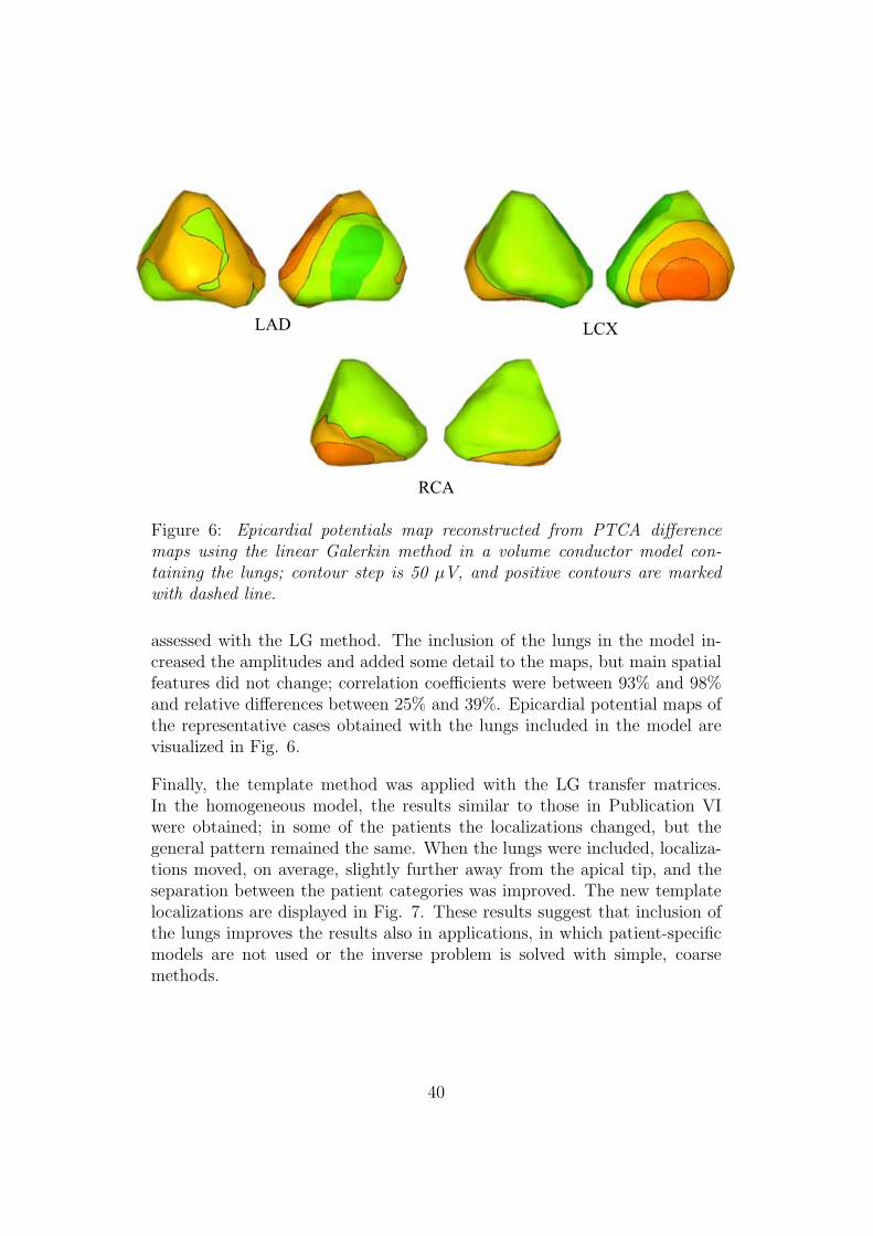
LAD LCX

RCA

Figure 6: Epicardial potentials map reconstructed from PTCA differencemaps using the linear Galerkin method in a volume conductor model con-taining the lungs; contour step is 50 μV, and positive contours are markedwith dashed line.

assessed with the LG method. The inclusion of the lungs in the model in-creased the amplitudes and added some detail to the maps, but main spatialfeatures did not change; correlation coefficients were between 93% and 98%and relative differences between 25% and 39%. Epicardial potential maps ofthe representative cases obtained with the lungs included in the model arevisualized in Fig. 6.

Finally, the template method was applied with the LG transfer matrices.In the homogeneous model, the results similar to those in Publication VIwere obtained; in some of the patients the localizations changed, but thegeneral pattern remained the same. When the lungs were included, localiza-tions moved, on average, slightly further away from the apical tip, and theseparation between the patient categories was improved. The new templatelocalizations are displayed in Fig. 7. These results suggest that inclusion ofthe lungs improves the results also in applications, in which patient-specificmodels are not used or the inverse problem is solved with simple, coarsemethods.

40

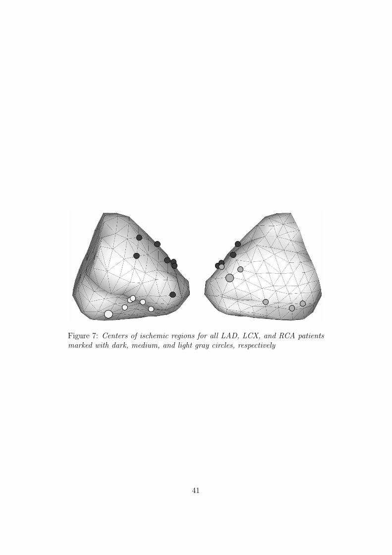
Figure 7: Centers of ischemic regions for all LAD, LCX, and RCA patientsmarked with dark, medium, and light gray circles, respectively

41

5 Summary and Outlook

In this Thesis, methods for solving the forward and inverse problems of elec-trocardiography were developed and applied to characterization of acute my-ocardial ischemia.

Basic methods for solving quasi-static potential-problems using the BEMwere collected to a Matlab toolbox. This Helsinki BEM library has been suc-cesful; it is currently in use in over 20 foreign research groups. In addition toelectrocardiographic problems, the methods in the library can be applied di-rectly to, e.g., electro- and magnetoencephalography, magnetocardiography,and electrostatic scattering. For the author, structures and routines of thelibrary have given a solid foundation for further method development.

Compared to conventionally used collocation methods, the linear Galerkin(LG) method was found to produce smaller forward-transfer and discretiza-tion errors in the epicardial potential problem. A good inverse solution needsan accurate forward solution as prerequisite; the use of the linear Galerkinmethod instead of the collocation method is thus, in general, recommended.But, when the inverse problem was solved using the traditional Tikhonovregularization, the LG method was, overall, not better than the other meth-ods. In most applications of epicardial potential imaging, the lungs havebeen omitted from the thoracic volume conductor model. If such a simpli-fication is done, the choice of basis and weighting functions is insignificant.The transfer matrix derived in this Thesis enables the inclusion of lungs inan easy-to-implement manner, without increasing the ill-posedness of theproblem. The quest for the accurate reconstruction of the epicardial poten-tial should thus head towards more accurate volume conductor models andmore advanced regularization techniques. The methodology developed in thisThesis can also be applied to reconstruction of cortical potential distributionfrom electroencephalographic data.

In the practical part of this Thesis, dipole modeling and epicardial potentialimaging were applied to detection, quantification, and localization of acutemyocardial ischemia. The results show that dipole modeling is an effectivetool for extracting main geometrical features from the body surface potentialmaps or from conventional ECG recordings: 21 of the 22 PTCA patients wereclassified correctly using the BSPM set, and 20 patients with a 5-electrodeset described elsewhere. Dipole-markers gave also encouraging results in de-tection and quantification of acute ischemia in a set of 79 patients and 84controls. Epicardial potential imaging characterized effectively the morpho-

43

logical features of the PTCA delta maps. The simple and robust templatemethod, developed in this Thesis, was able to localize the ischemic regionsanatomically correctly, although patient-specific volume conductor modelswere not used.

The method development carried out in this Thesis prepares the way for moreaccurate inverse reconstructions of epicardial potential. The results obtainedwith clinical datasets show that the modeling-approach can provide valuableinformation also without patient-specific models and complicated protocols.

44

References

[1] R.M. Gulrajani. Bioelectricity and Biomagnetism. Wiley and Sons,1998.

[2] P.W. MacFarlane. Lead systems. In P.W. MacFarlane and T.D.V.Lawrie, editors, Comprehensive Electrocardiography, pages 315–352.Pergamon Press, 1989.

[3] J.D. Jackson. Classical Electrodynamics. Wiley and Sons, 3rd edition,1999.

[4] R. Plonsey and D. Heppner. Considerations of quasistationarity in elec-trophysiological systems. Bull. Math. Biophys, 29:657–664, 1967.

[5] H.P. Schwan and C.F. Kay. Specific resistance of body tissues. Circ.Res., 4:664–670, 1956.

[6] H.C. Burger and R. van Dongen. Specific resistivity of body tissues.Phys. Med. Biol., 4:431–447, 1961.

[7] S. Rush, J.A. Abildskov, and R. McFee. Resistivity of body tissues atlow frequencies. Circ. Res., 12:40–50, 1963.

[8] S. Gabriel, R. W. Lau, and C. Gabriel. The dielectric properties ofbiological tissues: II. Measurements in the frequency range 10 Hz to 20GHz. Phys. Med. Biol., 41:2251–2269, 1996.

[9] H.P. Schwan and C.F. Kay. Capacitive properties of body tissues. Circ.Res., 5:439–443, 1957.

[10] H.P. Schwan and C.F. Kay. The conductivity of living tissues. Ann.N.Y. Acad. Sci., 65:1007–1013, 1957.

[11] M. Stenroos. Electrocardiographic Characterization of Myocardial Is-chemia with Numerical Field Calculation. Licentiate thesis, HelsinkiUniversity of Technology, 2005.

[12] J.G. Stinstra and M.J. Peters. The volume conductor may act as atemporal filter on the ECG and EEG. Med. Biol. Eng. Comp., 36:711–716, 1998.

[13] C.A. Brebbia and J. Dominguez. Boundary Elements: an IntroductoryCourse. McGraw–Hill, 1989.

45

[14] A.C.L. Barnard, I.M. Duck, and M.S. Lynn. The application of elec-tromagnetic theory to electrocardiology. I. Derivation of the integralequations. Biophys. J., 7:443–462, 1967.

[15] A.C.L. Barnard, I.M. Duck, M.S. Lynn, and W.P. Timlake. The ap-plication of electromagnetic theory in electrocardiology. II. Numericalsolution of the integral equations. Biophys. J., 7:463–490, 1967.

[16] N. Morita, N. Kumagai, and J.R. Mautz. Integral Equation Methods forElectromagnetics, pages 134–135. Artech House, 1990.

[17] B.M. Horacek and J.C. Clements. The inverse problem of electrocardio-graphy: A solution in terms of single- and double-layer sources on theepicardial surface. Math. Biosci., 144:119–154, 1997.

[18] B.M. Horacek. The Effect on Electrocardiographic Lead Vectors of Con-ductivity Inhomogeneities in the Human Torso. PhD thesis, DalhousieUniversity, 1971.

[19] D.B. Geselowitz. On bioelectric potentials in an inhomogeneous volumeconductor. Biophys. J., 7:1–11, 1967.

[20] A. van Oosterom and J. Strackee. The solid angle of a plane triangle.IEEE Trans. Biomed. Eng., BME-30:125–126, 1983.

[21] J.C. de Munck. A linear discretization of the volume conductor boundaryintegral equation using analytically integrated elements. IEEE Trans.Biomed. Eng., 39:986–989, 1992.

[22] R.D. Graglia. On the numerical integration of the linear shape functionstimes the 3-D Green’s function or its gradient on a plane triangle. IEEETrans. Antennas Propag., 41:1448–1455, 1993.

[23] S. Jarvenpaa, M. Taskinen, and P. Yla-Oijala. Singularity extractiontechnique for integral equations with higher order basis functions onplane triangles and tetrahedra. Int. J. Numer. Meth. Eng., 58:1149–1165, 2003.

[24] M.S. Lynn and W.P. Timlake. The use of multiple deflations in thenumerical solution of singular systems of equations, with applications topotential theory. SIAM J. Num. Anal., 5:303–322, 1968.

[25] G. Fischer, B. Tilg, F. Hanser, B. Messnarz, and P. Wach. On modelingthe Wilson terminal in the boundary and finite element method. IEEETrans. Biomed. Eng., 49:217–224, 2002.

46

[26] R.C. Barr, M. Ramsey, and M.S. Spach. Relating epicardial to bodysurface potential distributions by means of transfer coefficients basedon geometry measurements. IEEE Trans. Biomed. Eng., BME-24:1–11,1977.

[27] F. Greensite. Heart surface electrocardiographic inverse solutions. In BinHe, editor, Modeling and Imaging of Bioelectrical Activity: Principlesand Applications, pages 119–160. Kluwer Academic, 2004.

[28] H. Helmholtz. Ueber einige Gesetze der Vertheilung elektrischer Stromein korperlichen Leitern mit Anwendung auf die thierisch-elektrischenVersuche. Annalen der Physik und Chemie, 89:211–233; 353–377, 1853.

[29] J.T. Nenonen, M.S. Hamalainen, and R.J. Ilmoniemi. Minimum-normestimation in a boundary-element torso model. Med. Biol. Eng. Com-put., 32:43–48, 1994.

[30] W. Einthoven, G. Fahr, and A. de Waart. Uber die Richtung und diemanifeste Grosse der Potentialschwankungen in menschlichen Herzenund uber den Einfluss der Herzlage auf die Form des Elektrokardio-gramms. Pflugers Archivs fur Physiologie, 150:275–315, 1913.

[31] H.C. Burger and J.B. van Milaan. Heart-vector and leads. Brit. Heart.J., 8:157–161, 1946.

[32] H.C. Burger and J.B. van Milaan. Heart-vector and leads: Part II. Brit.Heart J., 9:154–160, 1947.

[33] H.C. Burger and J.B. van Milaan. Heart-vector and leads: Part III.Brit. Heart J., 10:229–233, 1948.

[34] B. Taccardi. Distribution of heart potentials on the thoracic surface ofnormal human subjects. Circ. Res., 12:341–352, 1963.

[35] E. Frank. An accurate, clinically practical system for spatial vectorcar-diography. Circulation, 13:737–749, 1956.

[36] R.E. Ideker, J.P. Bandura, R.A. Larsen, J.W. Cox, F.W. Keller, andD.A. Brody. Localization of heart vectors produced by epicardial burnsand ectopic stimuli; validation of a dipole ranging method. Circ. Res.,36:105–112, 1975.

[37] R.E. Ideker, J.P. Bandura, J.W. Cox, F.W. Keller, D.M. Mirvis, andD.A. Brody. Path and significance of heart vector migration during

47

QRS and ST–T complexes of ectopic beats in isolated perfused rabbithearts. Circ. Res., 41:558–564, 1977.

[38] P. Savard, F.A. Roberge, J.B. Perry, and R.A. Nadeau. Representationof cardiac electrical activity by a moving dipole for normal and ectopicbeats in the intact dog. Circ. Res., 46:415–425, 1980.

[39] D.M. Mirvis and M.A. Holbrook. Body surface distributions of repolar-ization potentials after acute myocardial infarction. III. Dipole rangingin normal subjects and in patients with acute myocardial infarction. J.Electrocardiol., 14:387–398, 1981.

[40] R.M. Gulrajani, H. Pham-Huy, R.A. Nadeau, P. Savard, J. de Guise,R.E. Primeau, and F.A. Roberge. Application of the single movingdipole inverse solution to the study of the Wolff–Parkinson–White syn-drome in man. J. Electrocardiol., 17:271–287, 1984.

[41] T.F. Oostendorp and A. van Oosterom. Source parameter estimationin inhomogeneous volume conductors of arbitrary shape. IEEE Trans.Biomed. Eng., 36:382–391, 1989.

[42] K. Pesola, J. Nenonen, R. Fenici, J. Lotjonen, M. Makijarvi, P. Fenici,P. Korhonen, K. Lauerma, M. Valkonen, L. Toivonen, and T. Katila.Bioelectromagnetic localization of a pacing catheter in the heart. Phys.Med. Biol, 44:2565–2578, 1999.

[43] A.A. Armoundas, A.B. Feldman, R. Mukkamala, B. He, T.J. Mullen,P.A. Belk, Y.Z. Lee, and R.J. Cohen. Statistical accuracy of a movingequivalent dipole method to identify sites of origin of cardiac electricactivation. IEEE Trans. Biomed. Eng., 50:1360–1370, 2003.

[44] Y. Fukuoka, T.F. Oostendorp, D.A. Sherman, and A.A. Armoundas.Applicability of the single equivalent moving dipole model in an infinitehomogeneous medium to identify cardiac electrical sources: A computersimulation study in a realistic anatomic geometry torso model. IEEETrans. Biomed. Eng., 53:2436–2444, 2006.

[45] M.E. Barley, A.A. Armoundas, K.J. Choppy, A.M Galea, G.B.Hirschmann, and R.J. Cohen. Demonstration of a novel catheter guid-ing method for the ablative therapy of ventricular tachycardia. Comput.Cardiol. 2006, 33:613–616, 2006.

48

[46] D. Gabor and C.V. Nelson. Determination of the resultant dipole of theheart from measurements on the body surface. J. Appl. Phys, 25:413–416, 1954.

[47] J. Nenonen, T. Katila, M. Leinio, J. Montonen, M. Makijarvi, and P. Sil-tanen. Magnetocardiographic functional localization using current mul-tipole models. IEEE Trans. Biomed. Eng., 38:648–657, 1991.

[48] R.M. Gulrajani, P. Savard, and F.A. Roberge. The inverse problem inelectrocardiology: solutions in terms of equivalent sources. Crit. Rev.Biomed. Eng., 16:171–214, 1988.

[49] J. Nenonen, K. Pesola, H. Hanninen, K. Lauerma, P. Takala, T. Makela,M. Makijarvi, J. Knuuti, L. Toivonen, and T. Katila. Current-densityestimation of exercise-induced ischemia in patients with multivessel coro-nary artery disease. J. Electrocardiol., 34 Suppl.:37–42, 2001.

[50] G. Huiskamp and A. van Oosterom. The depolarization sequence of thehuman heart surface computed from measured body surface potentials.IEEE Trans. Biomed. Eng., 35:1047–1058, 1988.

[51] D.B. Geselowitz. On the theory of the electrocardiogram. Proceedingsof the IEEE, 77:857–876, 1989.

[52] A. van Oosterom. Genesis of the T wave as based on an equivalentsurface source model. J. Electrocardiol., 36 Suppl.:217–227, 2001.

[53] A. van Oosterom and T.F. Oostendorp. ECGSIM: an interactive toolfor studying the genesis of QRST waveforms. Heart, 90:165–168, 2004.

[54] D.B. Geselowitz and W.T. Miller III. A bidomain model for anisotropiccardiac muscle. Ann. Biomed. Eng., 11:191–206, 1983.

[55] T. Berger, G. Fischer, B. Pfeifer, R. Modre, F. Hanser, T. Trieb, F.X.Roithinger, M. Stuhlinger, O. Pachinger, B. Tilg, and F. Hintringer.Single-beat noninvasive imaging of cardiac electrophysiology of ventric-ular pre-excitation. J. Amer. Coll. Cardiol., 48:2045–2054, 2006.

[56] R. Modre, B. Tilg, G. Fischer, F. Hanser, B. Messnarz, M. Seger, F. Hin-tringer, and F.X. Roithinger. Ventricular surface activation time imag-ing from electrocardiogram mapping data. Med. Biol. Eng. Comput.,42:146–150, 2004.

49

[57] B. Tilg, G. Fischer R. Modre, F. Hanser, B. Messnarz, and F.X.Roithinger. Electrocardiographic imaging of atrial and ventricular elec-trical activation. Med. Imag. Anal., 7:391–398, 2003.

[58] R. Modre, B. Tilg, G. Fischer, F. Hanser, B. Messnarz, M. Seger, M.F.H.Schocke, T. Berger, F. Hintringer, and F.X. Roithinger. Atrial noninva-sive activation mapping of paced rhythm data. J. Cardiovasc. Electro-physiol., 14:1–8, 2003.

[59] H.S. Oster, B. Taccardi, R.L. Lux, P.R. Ershler, and Y. Rudy. Noninva-sive electrocardiographic imaging: Reconstruction of epicardial poten-tials, electrograms, and isochrones and localization of single and multipleelectrocardiac events. Circulation, 96:1012–1024, 1997.

[60] C. Ramanathan, R.N. Ghanem, P. Jia, K. Ryu, and Y. Rudy. Non-invasive electrocardiographic imaging for cardiac electrophysiology andarrhythmia. Nature Med., 10:422–428, 2004.

[61] R.N. Ghanem, P. Jia, C. Ramanathan, K. Ruy, A. Markowitz, andY. Rudy. Noninvasive electrocardiographic imaging (ECGI): Compar-ison to intraoperative mapping in patients. Heart Rhythm, 2:339–354,2005.

[62] Y. Rudy and B.J. Messinger-Rapport. The inverse problem in electro-cardiography: Solutions on Terms of Epicardial Potentials. CRC Crit.Rev. Biomed. Eng., 16:215–268, 1988.

[63] R.S. MacLeod, M. Gardner, R.M. Miller, and B.M. Horacek. Applicationof an electrocardiographic inverse solution to localize ischemia duringcoronary angioplasty. J. Cardiovasc. Electrophysiol., 6:2–18, 1995.

[64] S. Ghosh and Y. Rudy. Accuracy of quadratic versus linear interpolationin noninvasive electrocardiographic imaging (ECGI). Ann. Biomed. Eng,33:1187–1201, 2005.

[65] P. Colli-Franzone, L. Guerri, S. Tentoni, C. Viganotti, S. Baruffi,S. Spaggiari, and B. Taccardi. A mathematical procedure for solvingthe inverse potential problem of electrocardiography. Analysis of thetime–space accuracy from in vitro experimental data. Math. Biosci.,77:353–396, 1984.

[66] A. Pullan. A high-order coupled finite element/boundary element torsomodel. IEEE Trans. Biomed. Eng., 43:292–298, 1996.

50

[67] Y. Wang and Y. Rudy. Application of the method of fundamental solu-tions to potential-based inverse electrocardiography. Ann. Biomed. Eng,34:1272–1288, 2006.

[68] A.S. Ferguson and G. Stroink. Factors affecting the accuracy of theboundary element method in the forward problem I: Calculating thesurface potentials. IEEE Trans. Biomed. Eng., 44:1139–1155, 1997.

[69] P.C. Stanley, T.C. Pilkington, and M.N. Morrow. The effects of tho-racic inhomogeneities on the relationship between epicardial and torsopotential. IEEE Trans. Biomed. Eng, BME-33:273–284, 1986.

[70] R.N. Klepfer, C.R. Johnson, and R.S. MacLeod. The effects of inho-mogeneities and anisotropies on electrocardiographic fields: A 3-D finiteelement study. IEEE Trans. Biomed. Eng., 44:706–719, 1997.

[71] C. Ramanathan and Y. Rudy. Electrocardiographic imaging: I. Effect oftorso inhomogeneities on body surface electrocardiographic potentials.J. Cardiovasc. Electrophysiol., 12:229–240, 2001.

[72] A. van Oosterom. The use of the spatial covariance in computing peri-cardial potentials. IEEE Trans. Biomed. Eng., 46:778–787, 1999.

[73] C. Ramanathan and Y. Rudy. Electrocardiographic imaging: II. Effectof torso inhomogeneities on noninvasive reconstruction of epicardial po-tentials, electrograms, and isochrones. J. Cardiovasc. Electrophysiol.,12:241–252, 2001.

[74] R. McFee and S. Rush. Qualitative effects of thoracic resistance variationon the interpretation of electrocardiograms: The low resistance surfacelayer. Am. Heart J., pages 48–61, 1968.

[75] R.S. MacLeod and D.H. Brooks. Validation approaches for electrocar-diographic inverse problems. In P. Johnston, editor, Advances in Com-putational Biomedicine (Volume 3), pages 229–268.

[76] M.P. Nash and A.J. Pullan. Challenges facing validation of noninvasiveelectrical imaging of the heart. Ann. Noninvasive Electrophysiol., 10:73–82, 2005.

[77] A.M. Katz. Physiology of the Heart. Raven Press, 2nd edition, 1992.

[78] D. Li, C.Y. Li, A.C. Yong, P.R. Johnston, and D. Kilpatrick. EpicardialST depression in acute myocardial infarction. Circ. Res., 85:959–964,1999.

51

[79] B. Hopenfeld, J.G. Stinstra, and R.S. MacLeod. Mechanism for STdepression associated with contiguous subendocardial ischemia. J. Car-diocasc. Electrophysiol., 15:1200–1206, 2004.

[80] B. Hopenfeld, J.G. Stinstra, and R.S. MacLeod. The effect of conduc-tivity on ST-segment epicardial potentials arising from subendocardialischemia. Ann. Biomed. Eng., 33:751–763, 2005.

[81] M.C. MacLachlan, J. Sundnes, and G.T. Lines. Simulation of ST seg-ment changes during subendocardial ischemia using a realistic 3-D car-diac geometry. IEEE Trans. Biomed. Eng., 52:799–807, 2005.

[82] M. Potse, R. Coronel, S. Falcao, A-R. LeBlanc, and A. Vinet. The effectof lesion size and tissue remodeling on ST deviation in partial-thicknessischemia. Heart Rhythm, 4:200–206, 2007.

[83] D. Li, C.Y. Li, A.C. Yong, and D. Kilpatrick. Source of electrocardio-graphic ST changes in subendocardial ischemia. Circ. Res., 82:925–970,1998.

[84] K. Thygesen, J.S. Alpert, and H.D. White; on behalf of the JointESC/ACCF/AHA/WHF Task Force for the redefinition of myocardialinfarction. Universal definition of myocardial infarction. Circulation,116:2634–2653, 2007.

[85] E. Pueyo, L. Sornmo, and P. Laguna. QRS slopes for detection andcharacterization of myocardial ischemia. IEEE Trans. Biomed. Eng.,55:468–477, 2008.

[86] J. Pettersson, O. Pahlm, E. Carro, L. Edenbrandt, M. Ringborn,L. Sornmo, S.G. Warren, and G.S. Wagner. Changes in high-frequencyQRS components are more sensitive than ST-deviation for detectingacute coronary artery occlusion. J. Amer. Coll. Cardiol, 36:1827–1834,2000.

[87] B.M. Horacek and G.S. Wagner. Electrocardiographic ST-segmentchanges during acute myocardial ischemia. Cardiac Electrophysiol. Rev.,6:196–203, 2002.

[88] F. Kornreich. Identification of best electrocardiographic leads for diag-nosing acute myocardial ischemia. J. Electrocardiol., 31 Suppl.:157–163,1998.

52

[89] S-F. Wung and B. Drew. Comparison of 18-lead ECG and selected bodysurface potential mapping leads in determining maximally deviated STlead and efficacy in detecting acute myocardial ischemia during coronaryocclusion. J. Electrocardiol., 32 Suppl.:30–36, 1999.

[90] R.S. MacLeod. Percutaneous Transluminal Coronary Angioplasty as aModel of Cardiac Ischemia: Clinical and Modelling Studies. PhD thesis,Dalhousie University, 1990.

[91] K. Simelius. Development of cardiographic mapping techniques for clin-ical use. Licentiate thesis, Helsinki University of Technology, 1998.

[92] A.M. Lincoff and E.J. Topol. Interventional catheterization techniques.In E. Braunwald, editor, Heart disease: a textbook of cardiovascularmedicine, pages 1366–1391. W.B. Saunders, 5th edition, 1997.

[93] Texas Heart Institute. Coronary artery disease.http://www.texasheart.org/HIC/Anatomy/coroanat.cfm, May2008.

[94] H. Vaananen, P. Korhonen, J. Montonen, M. Makijarvi, J. Nenonen,L. Oikarinen, K. Simelius, L. Toivonen, and T. Katila. Non-invasive ar-rhythmia risk evaluation in clinical environment. Herzschrittmacherther-apie und Elektrophysiologie, 11:229–234, 2000.

[95] T.F. Oostendorp, A. van Oosterom, and G. Huiskamp. Interpolation ona triangulated 3D surface. J. Comput. Phys., 80:331–343, 1989.

[96] P. Grande, B.F. Hansen, C. Christiansen, and J. Naestoft. Acute my-ocardial infarct size estimated by serum CK–MB determinations: Clin-ical accuracy and prognostic relevance utilizing a practical modificationof the isoenzyme approach. Amer. Heart J., 101:582–586, 1981.

[97] J. Carpenter and J. Bithell. Bootstrap confidence intervals: when,which, what? A practical guide for medical statisticians. Stat. Med.,19:1141–1164, 2000.

[98] B. Efron and R.J. Tibshirani. An Introduction to the Bootstrap. Chap-man and Hall, 1993.

53