Appendix

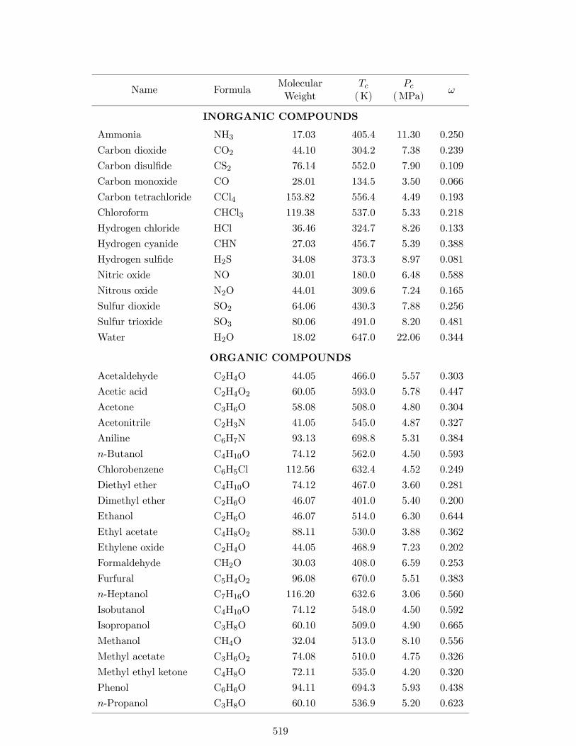
Appendix A

Critical Constants and Acentric Factors

Compiled from

1. NIST (National Institute of Standards and Technology) Chemistry WebBookwww.nist.gov/chemistry

2. Korea Thermophysical Properties Data Bank (KDB)www.cheric.org/research/kdb

517

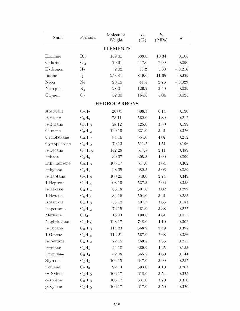
Name FormulaMolecularWeight

Tc(K)

Pc(MPa)

ω

ELEMENTS

Bromine Br2 159.81 588.0 10.34 0.108

Chlorine Cl2 70.91 417.0 7.99 0.090

Hydrogen H2 2.02 33.2 1.30 − 0.216Iodine I2 253.81 819.0 11.65 0.229

Neon Ne 20.18 44.4 2.76 − 0.029Nitrogen N2 28.01 126.2 3.40 0.039

Oxygen O2 32.00 154.6 5.04 0.025

HYDROCARBONS

Acetylene C2H2 26.04 308.3 6.14 0.190

Benzene C6H6 78.11 562.0 4.89 0.212

n-Butane C4H10 58.12 425.0 3.80 0.199

Cumene C9H12 120.19 631.0 3.21 0.326

Cyclohexane C6H12 84.16 554.0 4.07 0.212

Cyclopentane C5H10 70.13 511.7 4.51 0.196

n-Decane C10H22 142.28 617.8 2.11 0.489

Ethane C2H6 30.07 305.3 4.90 0.099

Ethylbenzene C8H10 106.17 617.0 3.64 0.302

Ethylene C2H4 28.05 282.5 5.06 0.089

n-Heptane C7H16 100.20 540.0 2.74 0.349

1-Heptene C7H14 98.19 537.3 2.92 0.358

n-Hexane C6H14 86.18 507.6 3.02 0.299

1-Hexene C6H14 84.16 504.0 3.21 0.285

Isobutane C4H10 58.12 407.7 3.65 0.183

Isopentane C5H12 72.15 461.0 3.38 0.227

Methane CH4 16.04 190.6 4.61 0.011

Naphthalene C10H8 128.17 748.0 4.10 0.302

n-Octane C8H18 114.23 568.9 2.49 0.398

1-Octene C8H16 112.21 567.0 2.68 0.386

n-Pentane C5H12 72.15 469.8 3.36 0.251

Propane C3H8 44.10 369.9 4.25 0.153

Propylene C3H6 42.08 365.2 4.60 0.144

Styrene C8H8 104.15 647.0 3.99 0.257

Toluene C7H8 92.14 593.0 4.10 0.263

m-Xylene C8H10 106.17 618.0 3.54 0.325

o-Xylene C8H10 106.17 631.0 3.70 0.310

p-Xylene C8H10 106.17 617.0 3.50 0.320

518

Name FormulaMolecularWeight

Tc(K)

Pc(MPa)

ω

INORGANIC COMPOUNDS

Ammonia NH3 17.03 405.4 11.30 0.250

Carbon dioxide CO2 44.10 304.2 7.38 0.239

Carbon disulfide CS2 76.14 552.0 7.90 0.109

Carbon monoxide CO 28.01 134.5 3.50 0.066

Carbon tetrachloride CCl4 153.82 556.4 4.49 0.193

Chloroform CHCl3 119.38 537.0 5.33 0.218

Hydrogen chloride HCl 36.46 324.7 8.26 0.133

Hydrogen cyanide CHN 27.03 456.7 5.39 0.388

Hydrogen sulfide H2S 34.08 373.3 8.97 0.081

Nitric oxide NO 30.01 180.0 6.48 0.588

Nitrous oxide N2O 44.01 309.6 7.24 0.165

Sulfur dioxide SO2 64.06 430.3 7.88 0.256

Sulfur trioxide SO3 80.06 491.0 8.20 0.481

Water H2O 18.02 647.0 22.06 0.344

ORGANIC COMPOUNDS

Acetaldehyde C2H4O 44.05 466.0 5.57 0.303

Acetic acid C2H4O2 60.05 593.0 5.78 0.447

Acetone C3H6O 58.08 508.0 4.80 0.304

Acetonitrile C2H3N 41.05 545.0 4.87 0.327

Aniline C6H7N 93.13 698.8 5.31 0.384

n-Butanol C4H10O 74.12 562.0 4.50 0.593

Chlorobenzene C6H5Cl 112.56 632.4 4.52 0.249

Diethyl ether C4H10O 74.12 467.0 3.60 0.281

Dimethyl ether C2H6O 46.07 401.0 5.40 0.200

Ethanol C2H6O 46.07 514.0 6.30 0.644

Ethyl acetate C4H8O2 88.11 530.0 3.88 0.362

Ethylene oxide C2H4O 44.05 468.9 7.23 0.202

Formaldehyde CH2O 30.03 408.0 6.59 0.253

Furfural C5H4O2 96.08 670.0 5.51 0.383

n-Heptanol C7H16O 116.20 632.6 3.06 0.560

Isobutanol C4H10O 74.12 548.0 4.50 0.592

Isopropanol C3H8O 60.10 509.0 4.90 0.665

Methanol CH4O 32.04 513.0 8.10 0.556

Methyl acetate C3H6O2 74.08 510.0 4.75 0.326

Methyl ethyl ketone C4H8O 72.11 535.0 4.20 0.320

Phenol C6H6O 94.11 694.3 5.93 0.438

n-Propanol C3H8O 60.10 536.9 5.20 0.623

519

Appendix B

Heat Capacity of Ideal Gases

Compiled from


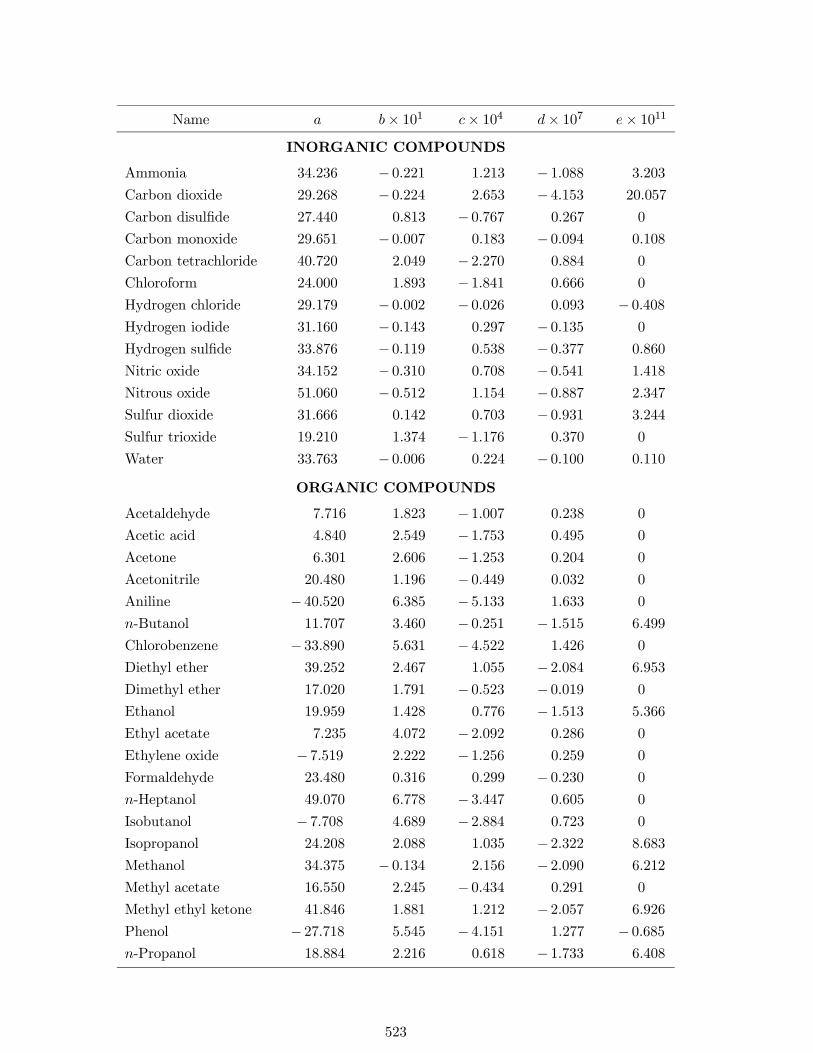
The heat capacity is expressed as a function of temperature in the form

eC∗P = a+ b T + c T 2 + dT 3 + e T 4

where eC∗P is in J/mol.K and T is in K. The coefficients are valid for 200K ≤ T ≤ 800K.

521

Name a b× 101 c× 104 d× 107 e× 1011

ELEMENTS

Bromine 33.860 0.113 − 0.119 453.400 0

Chlorine 26.468 0.340 − 0.373 0.159 − 0.172Hydrogen 27.004 0.119 − 0.241 0.215 − 0.615Iodine 35.590 0.065 − 0.070 0.028 0

Nitrogen 29.802 − 0.070 0.174 − 0.085 0.093

Oxygen 29.705 − 0.099 0.399 − 0.339 0.918

HYDROCARBONS

Acetylene 8.709 1.764 − 2.419 1.689 − 4.437Benzene − 60.711 6.267 − 5.795 2.799 − 5.493n-Butane 24.258 2.335 1.279 − 2.437 8.552

Cumene − 42.658 8.017 − 5.444 1.643 − 1.346Cyclohexane − 63.733 6.444 − 2.633 − 0.378 3.796

Cyclopentane − 61.877 5.809 − 3.631 1.020 − 0.770n-Decane 121.188 − 0.759 23.586 − 32.069 134.425

Ethane 33.313 − 0.111 3.566 − 3.762 11.983

Ethylbenzene 39.308 0.751 11.746 − 16.549 67.943

Ethylene 17.562 0.692 0.936 − 1.293 4.294

n-Heptane 37.663 3.941 2.587 − 4.744 16.635

1-Heptene 28.940 4.001 1.935 − 4.420 16.620

n-Hexane 32.365 3.447 2.026 − 3.806 13.306

Isobutane 24.108 2.091 2.166 − 3.372 11.619

Isopentane 4.817 4.159 − 0.809 − 1.008 4.688

Methane 36.155 − 0.511 2.215 − 1.824 4.899

Naphthalene − 47.760 7.213 − 3.873 − 0.012 4.422

n-Octane 37.209 4.810 2.419 − 5.167 18.845

1-Octene 33.168 4.544 2.477 − 5.425 20.411

n-Pentane 33.780 2.485 2.535 − 3.838 12.977

Propane 29.595 0.838 3.256 − 3.958 13.129

Propylene 17.905 1.478 68.773 − 1.384 4.845

Styrene − 51.641 7.580 − 6.943 3.422 − 7.005Toluene − 20.488 4.800 − 1.636 − 0.887 5.445

m-Xylene − 33.289 6.354 − 3.678 0.687 0.750

o-Xylene − 12.618 5.660 − 2.796 0.203 1.721

p-Xylene − 39.704 6.734 − 4.317 1.133 − 0.380

522

Name a b× 101 c× 104 d× 107 e× 1011

INORGANIC COMPOUNDS

Ammonia 34.236 − 0.221 1.213 − 1.088 3.203

Carbon dioxide 29.268 − 0.224 2.653 − 4.153 20.057

Carbon disulfide 27.440 0.813 − 0.767 0.267 0

Carbon monoxide 29.651 − 0.007 0.183 − 0.094 0.108

Carbon tetrachloride 40.720 2.049 − 2.270 0.884 0

Chloroform 24.000 1.893 − 1.841 0.666 0

Hydrogen chloride 29.179 − 0.002 − 0.026 0.093 − 0.408Hydrogen iodide 31.160 − 0.143 0.297 − 0.135 0

Hydrogen sulfide 33.876 − 0.119 0.538 − 0.377 0.860

Nitric oxide 34.152 − 0.310 0.708 − 0.541 1.418

Nitrous oxide 51.060 − 0.512 1.154 − 0.887 2.347

Sulfur dioxide 31.666 0.142 0.703 − 0.931 3.244

Sulfur trioxide 19.210 1.374 − 1.176 0.370 0

Water 33.763 − 0.006 0.224 − 0.100 0.110

ORGANIC COMPOUNDS

Acetaldehyde 7.716 1.823 − 1.007 0.238 0

Acetic acid 4.840 2.549 − 1.753 0.495 0

Acetone 6.301 2.606 − 1.253 0.204 0

Acetonitrile 20.480 1.196 − 0.449 0.032 0

Aniline − 40.520 6.385 − 5.133 1.633 0

n-Butanol 11.707 3.460 − 0.251 − 1.515 6.499

Chlorobenzene − 33.890 5.631 − 4.522 1.426 0

Diethyl ether 39.252 2.467 1.055 − 2.084 6.953

Dimethyl ether 17.020 1.791 − 0.523 − 0.019 0

Ethanol 19.959 1.428 0.776 − 1.513 5.366

Ethyl acetate 7.235 4.072 − 2.092 0.286 0

Ethylene oxide − 7.519 2.222 − 1.256 0.259 0

Formaldehyde 23.480 0.316 0.299 − 0.230 0

n-Heptanol 49.070 6.778 − 3.447 0.605 0

Isobutanol − 7.708 4.689 − 2.884 0.723 0

Isopropanol 24.208 2.088 1.035 − 2.322 8.683

Methanol 34.375 − 0.134 2.156 − 2.090 6.212

Methyl acetate 16.550 2.245 − 0.434 0.291 0

Methyl ethyl ketone 41.846 1.881 1.212 − 2.057 6.926

Phenol − 27.718 5.545 − 4.151 1.277 − 0.685n-Propanol 18.884 2.216 0.618 − 1.733 6.408

523

Appendix C

Antoine Constants

Compiled from

1. R.C. Reid, J.M. Prausnitz and T.K. Sherwood, The Properties of Gases and Liquids, 3rd

Ed., McGraw-Hill, New York, 1977.

The vapor pressure is expressed as a function of temperature in the form

lnP vap = A− B

T +C

where P vap is in bar and T is in K.

525

Name A B C Tmax Tmin

ELEMENTS

Argon 8.6128 700.51 − 5.84 94 81

Bromine 9.2239 2582.32 − 51.16 354 259

Chlorine 9.3408 1978.32 − 27.01 264 172

Hydrogen 7.0131 164.90 3.19 25 14

Nitrogen 8.3340 588.72 − 6.60 90 54

Oxygen 8.7873 734.55 − 6.45 100 63

HYDROCARBONS

Acetylene 9.7279 1637.14 − 19.77 202 194

Benzene 9.2806 2788.51 − 52.36 377 280

n-Butane 9.0580 2154.90 − 34.42 290 195

Cumene 9.3520 3363.60 − 63.37 454 311

Cyclohexane 9.1325 2766.63 − 50.50 380 280

Cyclopentane 9.2372 2588.48 − 41.79 345 230

n-Decane 9.3912 3456.80 − 78.67 476 330

Ethane 9.0435 1511.42 − 17.16 199 130

Ethylbenzene 9.3993 3279.47 − 59.95 450 300

Ethylene 8.9166 1347.01 − 18.15 182 120

n-Heptane 9.2535 2911.32 − 56.51 400 270

1-Heptene 9.2692 2895.51 − 53.97 400 265

n-Hexane 9.2164 2697.55 − 48.78 370 245

Isobutane 8.9179 2032.73 − 33.15 280 187

Isopentane 9.0136 2348.67 − 40.05 322 216

Methane 8.6041 597.84 − 7.16 120 93

Naphthalene 9.5224 3992.01 − 71.29 525 360

n-Octane 9.3224 3120.29 − 63.63 425 292

1-Octene 9.3428 3116.52 − 60.39 420 288

n-Pentane 9.2131 2477.07 − 39.94 330 220

Propane 9.1058 1872.46 − 25.16 249 164

Propylene 9.0825 1807.53 − 26.15 240 160

Styrene 9.3991 3328.57 − 63.72 460 305

Toluene 9.3935 3096.52 − 53.67 410 280

m-Xylene 9.5188 3366.99 − 58.04 440 300

o-Xylene 9.4954 3395.57 − 59.46 445 305

p-Xylene 9.4761 3346.65 − 57.84 440 300

526

Name A B C Tmax Tmin

INORGANIC COMPOUNDS

Ammonia 10.3729 2132.50 − 32.98 261 179

Carbon dioxide 15.9696 3103.39 − 0.16 204 154

Carbon disulfide 9.3642 2690.85 − 31.62 342 228

Carbon monoxide 7.7484 530.22 − 13.15 108 63

Carbon tetrachloride 9.2540 2808.19 − 45.99 374 253

Chloroform 8.3530 2696.79 − 46.16 370 260

Hydrogen chloride 9.8838 1714.25 − 14.45 200 137

Hydrogen sulfide 9.4838 1768.69 − 26.06 230 190

Nitric oxide 13.5112 1572.52 − 4.88 140 95

Nitrous oxide 9.5069 1506.49 − 25.99 200 144

Sulfur dioxide 10.1478 2302.35 − 35.97 280 195

Sulfur trioxide 14.2201 3995.70 − 36.66 332 290

Water 11.6834 3816.44 − 46.13 441 284

ORGANIC COMPOUNDS

Acetaldehyde 9.6729 2465.15 − 37.15 320 210

Acetic acid 10.1878 3405.57 − 56.34 430 290

Acetone 10.0311 2940.46 − 35.93 350 241

Acetonitrile 9.6672 2945.47 − 49.15 390 260

Aniline 10.0546 3857.52 − 73.15 500 340

n-Butanol 10.5958 3137.02 − 94.43 404 288

Chlorobenzene 9.4474 3295.12 − 55.60 420 320

Diethyl ether 9.4626 2511.29 − 41.95 340 225

Dimethyl ether 10.2265 2361.44 − 17.10 265 179

Ethanol 12.2917 3803.98 − 41.68 369 270

Ethyl acetate 9.5314 2790.50 − 57.15 385 260

Ethylene oxide 10.1198 2567.61 − 29.01 310 200

Formaldehyde 9.8573 2204.13 − 30.15 271 185

n-Heptanol 8.6866 2626.42 − 146.6 449 333

Isobutanol 10.2510 2874.73 − 100.3 388 293

Isopropanol 12.0727 3640.20 − 53.54 374 273

Methanol 11.9673 3626.55 − 34.29 364 257

Methyl acetate 9.5093 2601.92 − 56.15 360 245

Methyl ethyl ketone 9.9784 3150.42 − 36.65 376 257

Phenol 9.8077 3490.89 − 98.59 481 345

n-Propanol 10.9237 3166.28 − 80.15 400 285

527

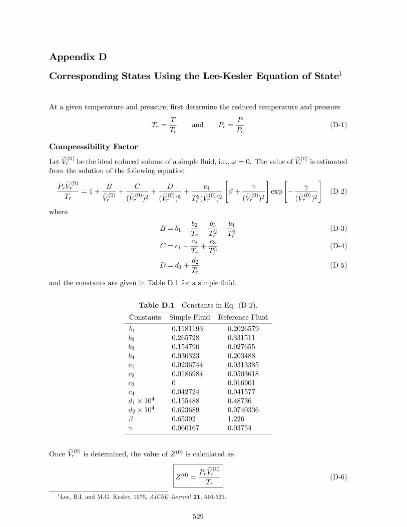
Appendix D

Corresponding States Using the Lee-Kesler Equation of State1

At a given temperature and pressure, first determine the reduced temperature and pressure

Tr =T

Tcand Pr =

P

Pc(D-1)

Compressibility Factor

Let eV (0)r be the ideal reduced volume of a simple fluid, i.e., ω = 0. The value of eV (0)r is estimatedfrom the solution of the following equation

Pr eV (0)r

Tr= 1 +

BeV (0)r

+C

(eV (0)r )2+

D

(eV (0)r )5+

c4

T 3r (eV (0)r )2

"β +

γ

(eV (0)r )2

#exp

"− γ

(eV (0)r )2

#(D-2)

where

B = b1 −b2Tr− b3

T 2r− b4

T 3r(D-3)

C = c1 −c2Tr+

c3T 3r

(D-4)

D = d1 +d2Tr

(D-5)

and the constants are given in Table D.1 for a simple fluid.

Table D.1 Constants in Eq. (D-2).

Constants Simple Fluid Reference Fluid

b1 0.1181193 0.2026579b2 0.265728 0.331511b3 0.154790 0.027655b4 0.030323 0.203488c1 0.0236744 0.0313385c2 0.0186984 0.0503618c3 0 0.016901c4 0.042724 0.041577d1 × 104 0.155488 0.48736d2 × 104 0.623689 0.0740336β 0.65392 1.226γ 0.060167 0.03754

Once eV (0)r is determined, the value of Z(0) is calculated as

Z(0) =Pr eV (0)r

Tr(D-6)

1Lee, B.I. and M.G. Kesler, 1975, AIChE Journal 21, 510-525.

529

For a reference fluid, the term eV (0)r in Eq. (D-2) is replaced by eV (R)r together with thereference fluid constants in Table D.1. Once the value of eV (R)r is determined from the solutionof Eq. (D-2), the value of Z(R) is calculated from

Z(R) =Pr eV (R)r

Tr(D-7)

Then, the value of Z(1) is given by

Z(1) =Z(R) − Z(0)

0.3978(D-8)

Enthalpy Departure Function

For a simple fluid³ eH − eHIG´(0)T,P

RTc= Tr

"Z(0) − 1− 1

Tr eV (0)r

µb2 +

2 b3Tr

+3 b4T 2r

¶− 1

2Tr(eV (0)r )2

µc2 −

3 c3T 2r

¶

+d2

5Tr(eV (0)r )5+ 3Eo

#(D-9)

where

Eo =c4

2T 3r γ

(β + 1−

"β + 1 +

γ

(eV (0)r )2

#exp

"− γ

(eV (0)r )2

#)(D-10)

For a reference fluid³ eH − eHIG´(R)T,P

RTc= Tr

"Z(R) − 1− 1

Tr eV (R)r

µb2 +

2 b3Tr

+3 b4T 2r

¶− 1

2Tr(eV (R)r )2

µc2 −

3 c3T 2r

¶

+d2

5Tr(eV (R)r )5+ 3ER

#(D-11)

where

ER =c4

2T 3r γ

(β + 1−

"β + 1 +

γ

(eV (R)r )2

#exp

"− γ

(eV (R)r )2

#)(D-12)

Then, the value of³ eH − eHIG

´(1)T,P

/RTc is given by

³ eH − eHIG´(1)T,P

RTc=

1

0.3978

⎡⎢⎢⎣³ eH − eHIG

´(R)T,P

RTc−

³ eH − eHIG´(0)T,P

RTc

⎤⎥⎥⎦ (D-13)

530

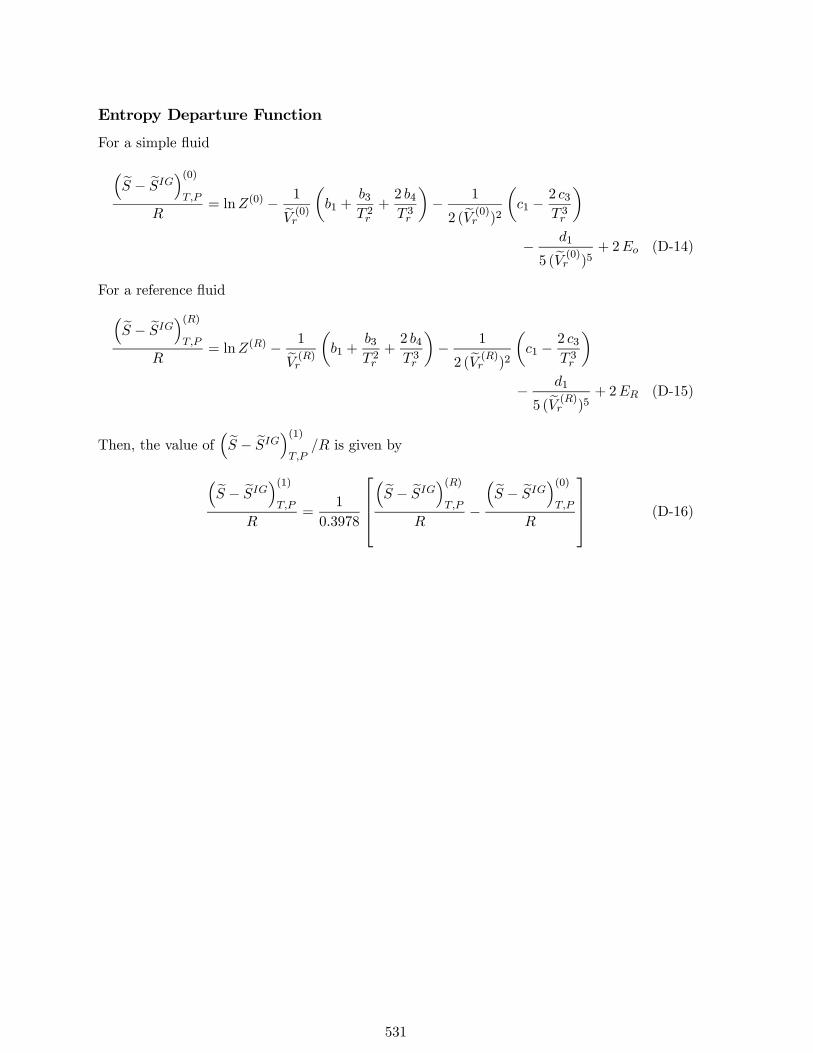
Entropy Departure Function

For a simple fluid³eS − eSIG´(0)T,P

R= lnZ(0) − 1eV (0)r

µb1 +

b3T 2r+2 b4T 3r

¶− 1

2 (eV (0)r )2

µc1 −

2 c3T 3r

¶− d1

5 (eV (0)r )5+ 2Eo (D-14)

For a reference fluid³eS − eSIG´(R)T,P

R= lnZ(R) − 1eV (R)r

µb1 +

b3T 2r+2 b4T 3r

¶− 1

2 (eV (R)r )2

µc1 −

2 c3T 3r

¶− d1

5 (eV (R)r )5+ 2ER (D-15)

Then, the value of³eS − eSIG

´(1)T,P

/R is given by

³eS − eSIG´(1)T,P

R=

1

0.3978

⎡⎢⎢⎣³eS − eSIG

´(R)T,P

R−

³eS − eSIG´(0)T,P

R

⎤⎥⎥⎦ (D-16)

531

Appendix E

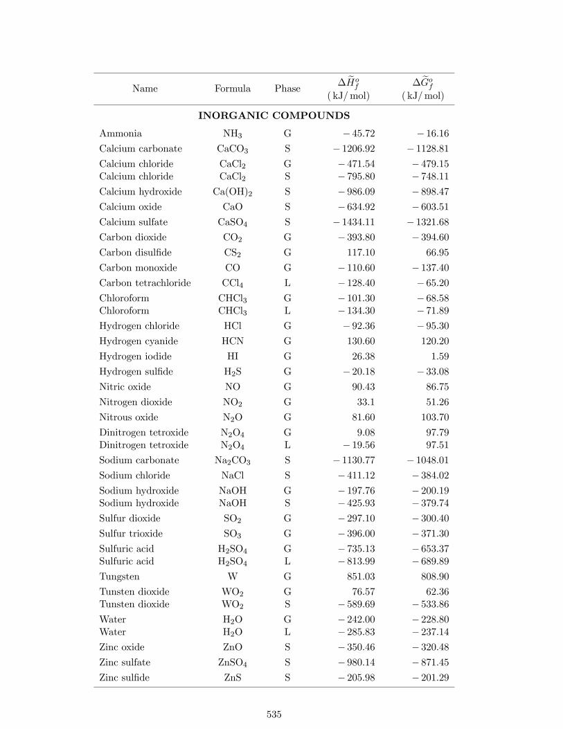
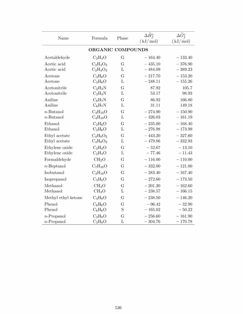
Enthalpy and Gibbs Energy of Formation at 298K and 1 bar

Compiled from

1. NIST (National Institute of Standards and Technology) Chemistry WebBookwww.nist.gov/chemistry


533

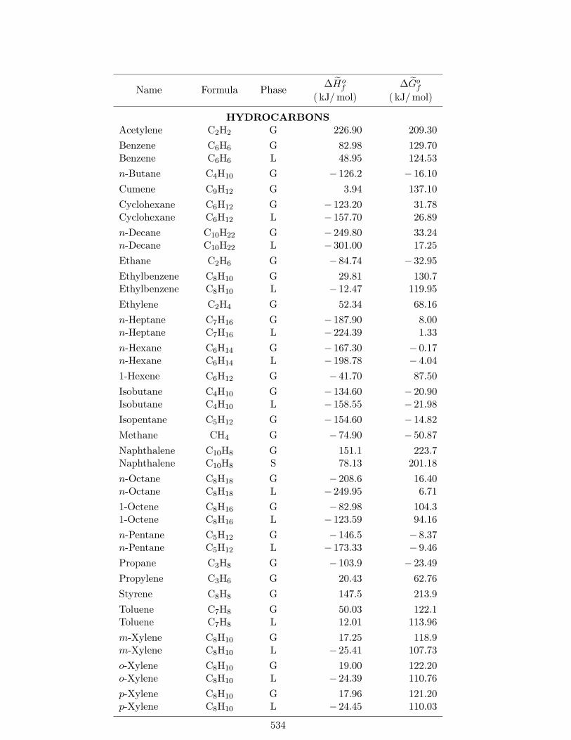
Name Formula Phase∆ eHo

f

( kJ/mol)

∆ eGof

( kJ/mol)

HYDROCARBONSAcetylene C2H2 G 226.90 209.30

Benzene C6H6 G 82.98 129.70Benzene C6H6 L 48.95 124.53

n-Butane C4H10 G − 126.2 − 16.10Cumene C9H12 G 3.94 137.10

Cyclohexane C6H12 G − 123.20 31.78Cyclohexane C6H12 L − 157.70 26.89

n-Decane C10H22 G − 249.80 33.24n-Decane C10H22 L − 301.00 17.25

Ethane C2H6 G − 84.74 − 32.95Ethylbenzene C8H10 G 29.81 130.7Ethylbenzene C8H10 L − 12.47 119.95

Ethylene C2H4 G 52.34 68.16

n-Heptane C7H16 G − 187.90 8.00n-Heptane C7H16 L − 224.39 1.33

n-Hexane C6H14 G − 167.30 − 0.17n-Hexane C6H14 L − 198.78 − 4.041-Hexene C6H12 G − 41.70 87.50

Isobutane C4H10 G − 134.60 − 20.90Isobutane C4H10 L − 158.55 − 21.98Isopentane C5H12 G − 154.60 − 14.82Methane CH4 G − 74.90 − 50.87Naphthalene C10H8 G 151.1 223.7Naphthalene C10H8 S 78.13 201.18

n-Octane C8H18 G − 208.6 16.40n-Octane C8H18 L − 249.95 6.71

1-Octene C8H16 G − 82.98 104.31-Octene C8H16 L − 123.59 94.16

n-Pentane C5H12 G − 146.5 − 8.37n-Pentane C5H12 L − 173.33 − 9.46Propane C3H8 G − 103.9 − 23.49Propylene C3H6 G 20.43 62.76

Styrene C8H8 G 147.5 213.9

Toluene C7H8 G 50.03 122.1Toluene C7H8 L 12.01 113.96

m-Xylene C8H10 G 17.25 118.9m-Xylene C8H10 L − 25.41 107.73

o-Xylene C8H10 G 19.00 122.20o-Xylene C8H10 L − 24.39 110.76

p-Xylene C8H10 G 17.96 121.20p-Xylene C8H10 L − 24.45 110.03

534


f

( kJ/mol)

∆ eGof

( kJ/mol)

INORGANIC COMPOUNDS

Ammonia NH3 G − 45.72 − 16.16Calcium carbonate CaCO3 S − 1206.92 − 1128.81Calcium chloride CaCl2 G − 471.54 − 479.15Calcium chloride CaCl2 S − 795.80 − 748.11Calcium hydroxide Ca(OH)2 S − 986.09 − 898.47Calcium oxide CaO S − 634.92 − 603.51Calcium sulfate CaSO4 S − 1434.11 − 1321.68Carbon dioxide CO2 G − 393.80 − 394.60Carbon disulfide CS2 G 117.10 66.95

Carbon monoxide CO G − 110.60 − 137.40Carbon tetrachloride CCl4 L − 128.40 − 65.20Chloroform CHCl3 G − 101.30 − 68.58Chloroform CHCl3 L − 134.30 − 71.89Hydrogen chloride HCl G − 92.36 − 95.30Hydrogen cyanide HCN G 130.60 120.20

Hydrogen iodide HI G 26.38 1.59

Hydrogen sulfide H2S G − 20.18 − 33.08Nitric oxide NO G 90.43 86.75

Nitrogen dioxide NO2 G 33.1 51.26

Nitrous oxide N2O G 81.60 103.70

Dinitrogen tetroxide N2O4 G 9.08 97.79Dinitrogen tetroxide N2O4 L − 19.56 97.51

Sodium carbonate Na2CO3 S − 1130.77 − 1048.01Sodium chloride NaCl S − 411.12 − 384.02Sodium hydroxide NaOH G − 197.76 − 200.19Sodium hydroxide NaOH S − 425.93 − 379.74Sulfur dioxide SO2 G − 297.10 − 300.40Sulfur trioxide SO3 G − 396.00 − 371.30Sulfuric acid H2SO4 G − 735.13 − 653.37Sulfuric acid H2SO4 L − 813.99 − 689.89Tungsten W G 851.03 808.90

Tunsten dioxide WO2 G 76.57 62.36Tunsten dioxide WO2 S − 589.69 − 533.86Water H2O G − 242.00 − 228.80Water H2O L − 285.83 − 237.14Zinc oxide ZnO S − 350.46 − 320.48Zinc sulfate ZnSO4 S − 980.14 − 871.45Zinc sulfide ZnS S − 205.98 − 201.29

535


f

( kJ/mol)

∆ eGof

( kJ/mol)

ORGANIC COMPOUNDS

Acetaldehyde C2H4O G − 164.40 − 133.40Acetic acid C2H4O2 G − 435.10 − 376.90Acetic acid C2H4O2 L − 484.09 − 389.23Acetone C3H6O G − 217.70 − 153.20Acetone C3H6O L − 248.11 − 155.26Acetonitrile C2H3N G 87.92 105.7Acetonitrile C2H3N L 53.17 98.93

Aniline C6H7N G 86.92 166.80Aniline C6H7N L 31.11 149.18

n-Butanol C4H10O G − 274.90 − 150.90n-Butanol C4H10O L − 326.03 − 161.19Ethanol C2H6O G − 235.00 − 168.40Ethanol C2H6O L − 276.98 − 173.99Ethyl acetate C4H8O2 G − 443.20 − 327.60Ethyl acetate C4H8O2 L − 479.86 − 332.93Ethylene oxide C2H4O G − 52.67 − 13.10Ethylene oxide C2H4O L − 77.46 − 11.43Formaldehyde CH2O G − 116.00 − 110.00n-Heptanol C7H16O G − 332.00 − 121.00Isobutanol C4H10O G − 283.40 − 167.40Isopropanol C3H8O G − 272.60 − 173.50Methanol CH4O G − 201.30 − 162.60Methanol CH4O L − 238.57 − 166.15Methyl ethyl ketone C4H8O G − 238.50 − 146.20Phenol C6H6O G − 96.42 − 32.90Phenol C6H6O S − 165.02 − 50.22n-Propanol C3H8O G − 256.60 − 161.90n-Propanol C3H8O L − 304.76 − 170.78

536

Appendix F

Matrices

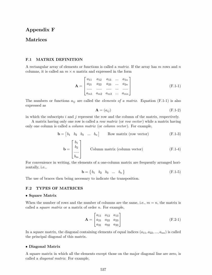
F.1 MATRIX DEFINITION

A rectangular array of elements or functions is called a matrix. If the array has m rows and ncolumns, it is called an m× n matrix and expressed in the form

A =

⎡⎢⎢⎣a11 a12 a13 ... a1na21 a22 a23 ... a2n..... ..... ..... ... .....am1 am2 am3 ... amn

⎤⎥⎥⎦ (F.1-1)

The numbers or functions aij are called the elements of a matrix. Equation (F.1-1) is alsoexpressed as

A = (aij) (F.1-2)

in which the subscripts i and j represent the row and the column of the matrix, respectively.A matrix having only one row is called a row matrix (or row vector) while a matrix having

only one column is called a column matrix (or column vector). For example,

b =£b1 b2 b3 ... bn

¤Row matrix (row vector) (F.1-3)

b =

⎡⎢⎢⎣b1b2.....bm

⎤⎥⎥⎦ Column matrix (column vector) (F.1-4)

For convenience in writing, the elements of a one-column matrix are frequently arranged hori-zontally, i.e.,

b =©b1 b2 b3 ... bn

ª(F.1-5)

The use of braces then being necessary to indicate the transposition.

F.2 TYPES OF MATRICES

• Square Matrix

When the number of rows and the number of columns are the same, i.e., m = n, the matrix iscalled a square matrix or a matrix of order n. For example,

A =

⎡⎣a11 a12 a13a21 a22 a23a31 a32 a33

⎤⎦ (F.2-1)

In a square matrix, the diagonal containing elements of equal indices (a11, a22, ..., ann) is calledthe principal diagonal of this matrix.

• Diagonal Matrix

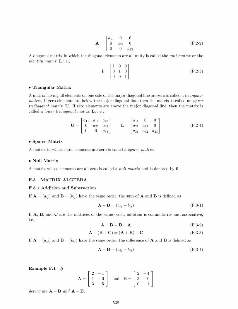
A square matrix in which all the elements except those on the major diagonal line are zero, iscalled a diagonal matrix. For example,

537

A =

⎡⎣a11 0 00 a22 00 0 a33

⎤⎦ (F.2-2)

A diagonal matrix in which the diagonal elements are all unity is called the unit matrix or theidentity matrix, I, i.e.,

I =

⎡⎣1 0 00 1 00 0 1

⎤⎦ (F.2-3)

• Triangular Matrix

A matrix having all elements on one side of the major diagonal line are zero is called a triangularmatrix. If zero elements are below the major diagonal line, then the matrix is called an uppertridiagonal matrix, U. If zero elements are above the major diagonal line, then the matrix iscalled a lower tridiagonal matrix, L, i.e.,

U =

⎡⎣a11 a12 a130 a22 a230 0 a33

⎤⎦ L =

⎡⎣a11 0 0a21 a22 0a31 a32 a33

⎤⎦ (F.2-4)

• Sparse Matrix

A matrix in which most elements are zero is called a sparse matrix.

• Null Matrix

A matrix whose elements are all zero is called a null matrix and is denoted by 0.

F.3 MATRIX ALGEBRA

F.3.1 Addition and Subtraction

If A = (aij) and B = (bij) have the same order, the sum of A and B is defined as

A+B = (aij + bij) (F.3-1)

If A, B, and C are the matrices of the same order, addition is commutative and associative,i.e.,

A+B = B+A (F.3-2)

A+ (B+C) = (A+B) +C (F.3-3)

If A = (aij) and B = (bij) have the same order, the difference of A and B is defined as

A−B = (aij − bij) (F.3-4)

Example F.1 If

A =

⎡⎣ 2 − 11 03 5

⎤⎦ and B =

⎡⎣ 2 − 43 00 1

⎤⎦determine A+B and A−B.

538

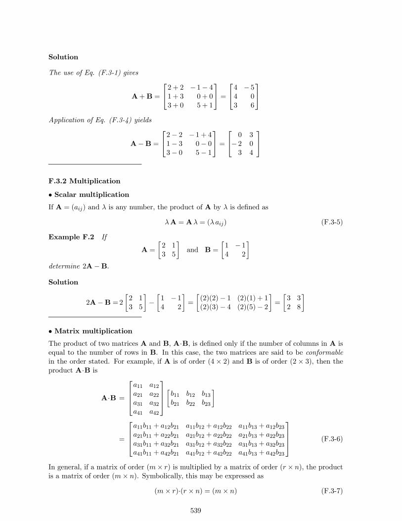
Solution

The use of Eq. (F.3-1) gives

A+B =

⎡⎣2 + 2 − 1− 41 + 3 0 + 03 + 0 5 + 1

⎤⎦ =⎡⎣4 − 54 03 6

⎤⎦Application of Eq. (F.3-4) yields

A−B =

⎡⎣2− 2 − 1 + 41− 3 0− 03− 0 5− 1

⎤⎦ =⎡⎣ 0 3− 2 03 4

⎤⎦

F.3.2 Multiplication

• Scalar multiplicationIf A = (aij) and λ is any number, the product of A by λ is defined as

λA = Aλ = (λaij) (F.3-5)

Example F.2 If

A =

∙2 13 5

¸and B =

∙1 − 14 2

¸determine 2A−B.

Solution

2A−B =2∙2 13 5

¸−∙1 − 14 2

¸=

∙(2)(2)− 1 (2)(1) + 1(2)(3)− 4 (2)(5)− 2

¸=

∙3 32 8

¸

• Matrix multiplicationThe product of two matrices A and B, A·B, is defined only if the number of columns in A isequal to the number of rows in B. In this case, the two matrices are said to be conformablein the order stated. For example, if A is of order (4 × 2) and B is of order (2 × 3), then theproduct A·B is

A·B =

⎡⎢⎢⎣a11 a12a21 a22a31 a32a41 a42

⎤⎥⎥⎦∙b11 b12 b13b21 b22 b23

¸

=

⎡⎢⎢⎣a11b11 + a12b21 a11b12 + a12b22 a11b13 + a12b23a21b11 + a22b21 a21b12 + a22b22 a21b13 + a22b23a31b11 + a32b21 a31b12 + a32b22 a31b13 + a32b23a41b11 + a42b21 a41b12 + a42b22 a41b13 + a42b23

⎤⎥⎥⎦ (F.3-6)

In general, if a matrix of order (m× r) is multiplied by a matrix of order (r× n), the productis a matrix of order (m× n). Symbolically, this may be expressed as

(m× r)·(r × n) = (m× n) (F.3-7)

539

Example F.3 If

A =

⎡⎣ 1 − 12 0− 1 5

⎤⎦ and B =

∙12

¸determine A·B.

Solution

A·B =

⎡⎣ 1 − 12 0− 1 5

⎤⎦∙12

¸

=

⎡⎣ (1)(1) + (−1)(2)(2)(1) + (0)(2)(−1)(1) + (5)(2)

⎤⎦ =⎡⎣− 12

9

⎤⎦

A matrix A can be multiplied by itself if and only if it is a square matrix. The productA·A can be expressed as A2. If the relevant products are defined, multiplication of matricesis associative, i.e.,

A·(B·C) = (A·B)·C (F.3-8)

and distributive, i.e.,A·(B+C) = A·B+A·C (F.3-9)

(B+C)·A = B·A+C·A (F.3-10)

but, in general, not commutative, i.e., A·B 6= B·A. For example, if A is of order (m×n) andB is of order (n×m), then the product A·B = C is a matrix of order (m×m). On the otherhand, the product B·A = D is a matrix of order (n × n). Even if the matrices A and B aresquare matrices of the same order, in general, C will be different from D.

For any unit (or identity) matrix I

I·A = A·I = A (F.3-11)

F.3.3 Some Properties of Matrices

• Any row (or column) in a matrix can be modified by multipliying or dividing by a nonzeroscalar without affecting the matrix.

• Any row (or column) can be added or subtracted from another row (or column) withoutaffecting the matrix.

• Any two rows (or columns) can be interchanged without affecting the matrix.

F.4 DETERMINANTS

For each square matrix A, it is possible to associate a scalar quantity called the determinantof A, |A|. If the matrix A in Eq. (F.1-1) is a square matrix, then the determinant of A isgiven by

|A| =

¯̄̄̄¯̄̄̄ a11 a12 a13 ... a1na21 a22 a23 ... a2n..... ..... ..... ... .....an1 an2 an3 ... ann

¯̄̄̄¯̄̄̄ (F.4-1)

540

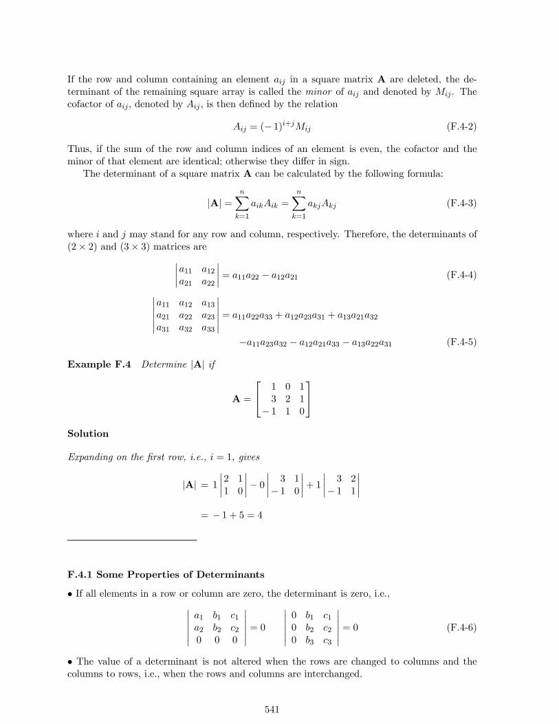
If the row and column containing an element aij in a square matrix A are deleted, the de-terminant of the remaining square array is called the minor of aij and denoted by Mij . Thecofactor of aij , denoted by Aij , is then defined by the relation

Aij = (− 1)i+jMij (F.4-2)

Thus, if the sum of the row and column indices of an element is even, the cofactor and theminor of that element are identical; otherwise they differ in sign.

The determinant of a square matrix A can be calculated by the following formula:

|A| =nX

k=1

aikAik =nX

k=1

akjAkj (F.4-3)

where i and j may stand for any row and column, respectively. Therefore, the determinants of(2× 2) and (3× 3) matrices are¯̄̄̄

a11 a12a21 a22

¯̄̄̄= a11a22 − a12a21 (F.4-4)

¯̄̄̄¯̄a11 a12 a13a21 a22 a23a31 a32 a33

¯̄̄̄¯̄ = a11a22a33 + a12a23a31 + a13a21a32

−a11a23a32 − a12a21a33 − a13a22a31 (F.4-5)

Example F.4 Determine |A| if

A =

⎡⎣ 1 0 13 2 1− 1 1 0

⎤⎦Solution

Expanding on the first row, i.e., i = 1, gives

|A| = 1

¯̄̄̄2 11 0

¯̄̄̄− 0

¯̄̄̄3 1− 1 0

¯̄̄̄+ 1

¯̄̄̄3 2− 1 1

¯̄̄̄= − 1 + 5 = 4

F.4.1 Some Properties of Determinants

• If all elements in a row or column are zero, the determinant is zero, i.e.,¯̄̄̄¯̄ a1 b1 c1a2 b2 c20 0 0

¯̄̄̄¯̄ = 0

¯̄̄̄¯̄ 0 b1 c10 b2 c20 b3 c3

¯̄̄̄¯̄ = 0 (F.4-6)

• The value of a determinant is not altered when the rows are changed to columns and thecolumns to rows, i.e., when the rows and columns are interchanged.

541

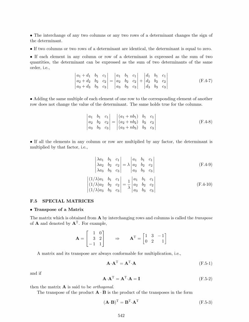
• The interchange of any two columns or any two rows of a determinant changes the sign ofthe determinant.

• If two columns or two rows of a determinant are identical, the determinant is equal to zero.• If each element in any column or row of a determinant is expressed as the sum of twoquantities, the determinant can be expressed as the sum of two determinants of the sameorder, i.e., ¯̄̄̄

¯̄a1 + d1 b1 c1a2 + d2 b2 c2a3 + d3 b3 c3

¯̄̄̄¯̄ =

¯̄̄̄¯̄a1 b1 c1a2 b2 c2a3 b3 c3

¯̄̄̄¯̄+

¯̄̄̄¯̄d1 b1 c1d2 b2 c2d3 b3 c3

¯̄̄̄¯̄ (F.4-7)

• Adding the same multiple of each element of one row to the corresponding element of anotherrow does not change the value of the determinant. The same holds true for the columns.

¯̄̄̄¯̄a1 b1 c1a2 b2 c2a3 b3 c3

¯̄̄̄¯̄ =

¯̄̄̄¯̄ (a1 + nb1) b1 c1(a2 + nb2) b2 c2(a3 + nb3) b3 c3

¯̄̄̄¯̄ (F.4-8)

• If all the elements in any column or row are multiplied by any factor, the determinant ismultiplied by that factor, i.e.,

¯̄̄̄¯̄λa1 b1 c1λa2 b2 c2λa3 b3 c3

¯̄̄̄¯̄ = λ

¯̄̄̄¯̄a1 b1 c1a2 b2 c2a3 b3 c3

¯̄̄̄¯̄ (F.4-9)

¯̄̄̄¯̄ (1/λ)a1 b1 c1(1/λ)a2 b2 c2(1/λ)a3 b3 c3

¯̄̄̄¯̄ = 1

λ

¯̄̄̄¯̄a1 b1 c1a2 b2 c2a3 b3 c3

¯̄̄̄¯̄ (F.4-10)

F.5 SPECIAL MATRICES

• Transpose of a Matrix

The matrix which is obtained fromA by interchanging rows and columns is called the transposeof A and denoted by AT. For example,

A =

⎡⎣ 1 03 2− 1 1

⎤⎦ ⇒ AT =

∙1 3 − 10 2 1

¸

A matrix and its transpose are always conformable for multiplication, i.e.,

A·AT = AT·A (F.5-1)

and ifA·AT = AT·A = I (F.5-2)

then the matrix A is said to be orthogonal.The transpose of the product A ·B is the product of the transposes in the form

(A·B)T = BT·AT (F.5-3)

542

• Symmetric and Skew-Symmetric Matrices

A square matrix A is said to be symmetric if

A = AT or aij = aji (F.5-4)

A square matrix A is said to be skew-symmetric (or antisymmetric) if

A = −AT or aij = −aji (F.5-5)

Equation (F.5-5) implies that the diagonal elements of a skew-symmetric matrix are all zero.

• Singular Matrix

A square matrix A for which the determinant |A| of its elements is zero, is termed a singularmatrix. If |A| 6= 0, then A is nonsingular.

• Inverse of a Matrix

If the determinant |A| of a square matrix A does not vanish, i.e., nonsingular matrix, it thenpossesses an inverse (or, reciprocal) matrix A−1 such that

A·A−1 = A−1·A = I (F.5-6)

The inverse of a matrix A is defined by

A−1 =AdjA|A| (F.5-7)

where AdjA is called the adjoint of A. It is obtained from a square matrix A by replacingeach element by its cofactor and then interchanging rows and columns.

Example F.5 Find the inverse of the matrix A given in Example F.4.

Solution

The minor of A is given by

Mij =

⎡⎢⎢⎢⎢⎢⎢⎢⎢⎢⎢⎣

¯̄̄̄2 11 0

¯̄̄̄ ¯̄̄̄3 1− 1 0

¯̄̄̄ ¯̄̄̄3 2− 1 1

¯̄̄̄¯̄̄̄0 11 0

¯̄̄̄ ¯̄̄̄1 1− 1 0

¯̄̄̄ ¯̄̄̄1 0− 1 1

¯̄̄̄¯̄̄̄0 12 1

¯̄̄̄ ¯̄̄̄1 13 1

¯̄̄̄ ¯̄̄̄1 03 2

¯̄̄̄

⎤⎥⎥⎥⎥⎥⎥⎥⎥⎥⎥⎦=

⎡⎣− 1 1 5− 1 1 1− 2 − 2 2

⎤⎦

The cofactor matrix is

Aij =

⎡⎣− 1 − 1 51 1 − 1− 2 2 2

⎤⎦The transpose of the cofactor matrix gives the adjoint of A as

AdjA =

⎡⎣− 1 1 − 2− 1 1 25 − 1 2

⎤⎦543

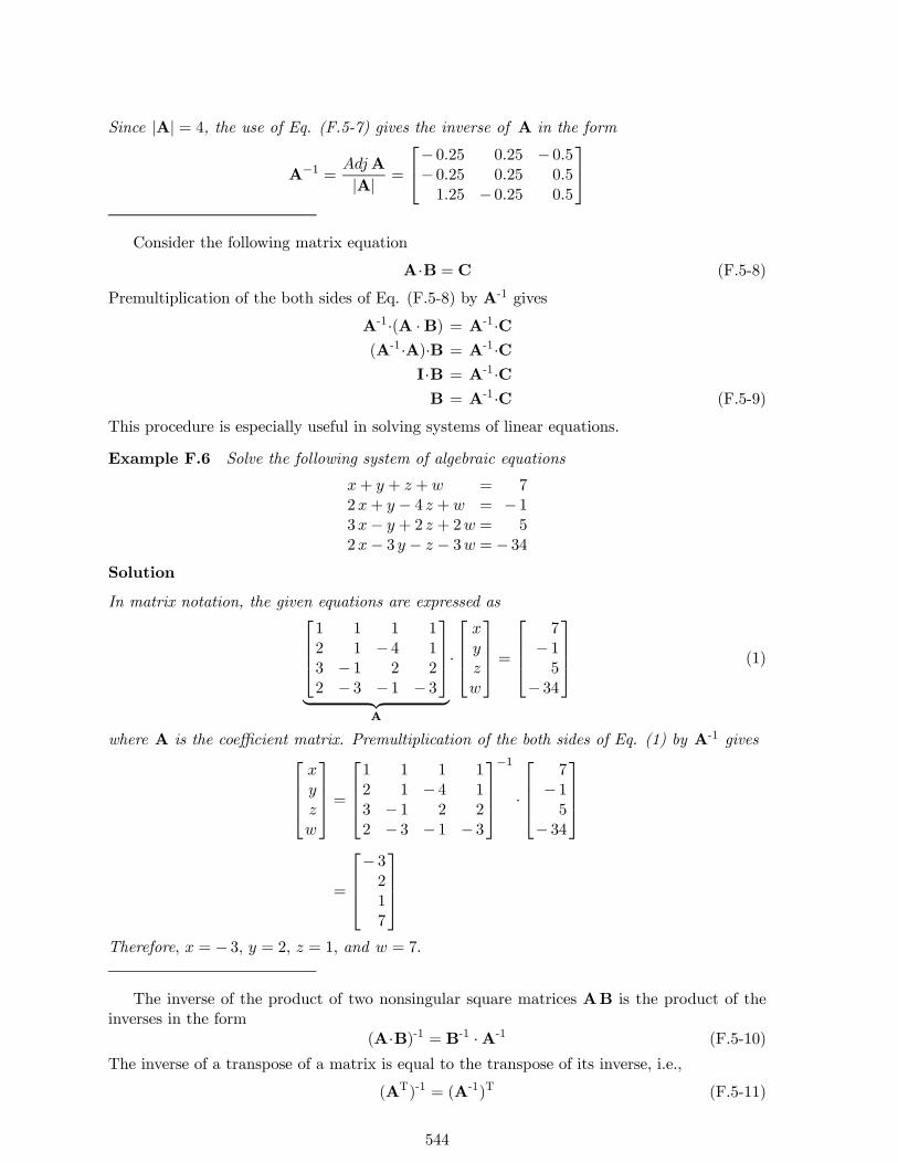
Since |A| = 4, the use of Eq. (F.5-7) gives the inverse of A in the form

A−1 =AdjA

|A| =

⎡⎣− 0.25 0.25 − 0.5− 0.25 0.25 0.51.25 − 0.25 0.5

⎤⎦Consider the following matrix equation

A·B = C (F.5-8)

Premultiplication of the both sides of Eq. (F.5-8) by A-1 gives

A-1·(A ·B) = A-1·C(A-1·A)·B = A-1·C

I·B = A-1·CB = A-1·C (F.5-9)

This procedure is especially useful in solving systems of linear equations.

Example F.6 Solve the following system of algebraic equations

x+ y + z +w = 72x+ y − 4 z + w = − 13x− y + 2 z + 2w = 52x− 3 y − z − 3w = − 34

Solution

In matrix notation, the given equations are expressed as⎡⎢⎢⎣1 1 1 12 1 − 4 13 − 1 2 22 − 3 − 1 − 3

⎤⎥⎥⎦| {z }

A

·

⎡⎢⎢⎣xyzw

⎤⎥⎥⎦ =⎡⎢⎢⎣

7− 15

− 34

⎤⎥⎥⎦ (1)

where A is the coefficient matrix. Premultiplication of the both sides of Eq. (1) by A-1 gives⎡⎢⎢⎣xyzw

⎤⎥⎥⎦ =⎡⎢⎢⎣1 1 1 12 1 − 4 13 − 1 2 22 − 3 − 1 − 3

⎤⎥⎥⎦−1

·

⎡⎢⎢⎣7− 15

− 34

⎤⎥⎥⎦

=

⎡⎢⎢⎣− 3217

⎤⎥⎥⎦Therefore, x = − 3, y = 2, z = 1, and w = 7.

The inverse of the product of two nonsingular square matrices AB is the product of theinverses in the form

(A·B)-1 = B-1 ·A-1 (F.5-10)

The inverse of a transpose of a matrix is equal to the transpose of its inverse, i.e.,

(AT)-1 = (A-1)T (F.5-11)

544

F.6 LINEAR DEPENDENCE

Consider the x-y coordinate system as shown in Figure F.1.

y is independent of x

x is independent of y

x

y

Figure F.1 Cartesian coordinate system.

The linear combination of x and y is expressed as λ1x + λ2y, where λ1 and λ2 are nonzeroscalars. Let the linear combination of x and y be equal to zero, i.e.,

λ1 x+ λ2 y = 0 (F.6-1)

Note that y = 0 on the x-axis, and Eq. (F.6-1) gives

λ1 x = 0 (F.6-2)

Since Eq. (F.6-2) must hold for any x, then λ1 = 0. On the other hand, x = 0 on the y-axisand Eq. (F.6-1) reduces to

λ2 y = 0 (F.6-3)

Since Eq. (F.6-3) must hold for any y, then λ2 = 0. Therefore, when x and y are independent,then the only set of multipliers λ1 and λ2 which will make λ1x+ λ2y = 0 are λ1 = λ2 = 0.

On the other hand, let us consider the case in which y is related to x through the followingrelationship

y = mx (F.6-4)

When the linear combination of x and y is equal to zero, Eq. (F.6-1) is still valid. Substitutionof Eq. (F.6-4) into Eq. (F.6-1) gives

(λ1 +mλ2)x = 0 ⇒ λ1 +mλ2 = 0 ⇒ λ1 = −mλ2 (F.6-5)

Therefore, when x and y are dependent, the equation λ1x + λ2y = 0 is satisfied whenλ1 = −mλ2.

F.6.1 Rank of a Matrix

Let A be a matrix of order (m× n) in which m is less than n. The determinants formed fromthe m rows and any m of the n columns are called minors of the matrix A.

The rank of a matrix, denoted by rank(A), is equal to the order of the highest ordernonvanishing minor. For a square matrix of order (n×n), the first minor will be the determinantof the matrix and of order n. The second minor will be of order (n−1), and so on to the minorof order 1.

Example F.7 Determine the rank of the matrix⎡⎣2 − 3 13 1 35 − 2 4

⎤⎦545

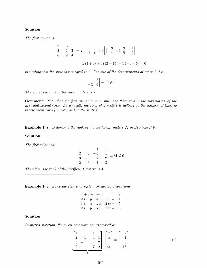
Solution

The first minor is ¯̄̄̄¯̄2 − 3 13 1 35 − 2 4

¯̄̄̄¯̄ = 2

¯̄̄̄1 3− 2 4

¯̄̄̄+ 3

¯̄̄̄3 35 4

¯̄̄̄+ 1

¯̄̄̄3 15 − 2

¯̄̄̄

= 2 (4 + 6) + 3 (12− 15) + 1 (− 6− 5) = 0

indicating that the rank is not equal to 3. For one of the determinants of order 2, i.e.,¯̄̄̄1 3− 2 4

¯̄̄̄= 10 6= 0

Therefore, the rank of the given matrix is 2.

Comment: Note that the first minor is zero since the third row is the summation of thefirst and second rows. As a result, the rank of a matrix is defined as the number of linearlyindependent rows (or columns) in the matrix.

Example F.8 Determine the rank of the coefficient matrix A in Example F.6.

Solution

The first minor is ¯̄̄̄¯̄̄̄1 1 1 12 1 − 4 13 − 1 2 22 − 3 − 1 − 3

¯̄̄̄¯̄̄̄ = 81 6= 0

Therefore, the rank of the coefficient matrix is 4.

Example F.9 Solve the following system of algebraic equations

x+ y + z + w = 72x+ y − 4 z + w = − 13x− y + 2 z + 2w = 52x− y + 7 z + 2w = 13

Solution

In matrix notation, the given equations are expressed as⎡⎢⎢⎣1 1 1 12 1 − 4 13 − 1 2 22 − 1 7 2

⎤⎥⎥⎦| {z }

A

·

⎡⎢⎢⎣xyzw

⎤⎥⎥⎦ =⎡⎢⎢⎣

7− 1513

⎤⎥⎥⎦ (1)

546

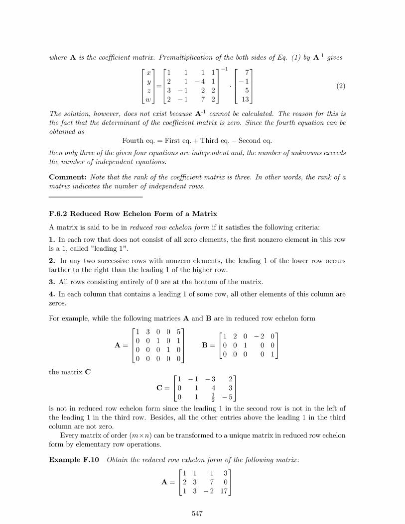
where A is the coefficient matrix. Premultiplication of the both sides of Eq. (1) by A-1 gives⎡⎢⎢⎣xyzw

⎤⎥⎥⎦=⎡⎢⎢⎣1 1 1 12 1 − 4 13 − 1 2 22 − 1 7 2

⎤⎥⎥⎦−1

·

⎡⎢⎢⎣7− 1513

⎤⎥⎥⎦ (2)

The solution, however, does not exist because A-1 cannot be calculated. The reason for this isthe fact that the determinant of the coefficient matrix is zero. Since the fourth equation can beobtained as

Fourth eq. = First eq.+Third eq.− Second eq.then only three of the given four equations are independent and, the number of unknowns exceedsthe number of independent equations.

Comment: Note that the rank of the coefficient matrix is three. In other words, the rank of amatrix indicates the number of independent rows.

F.6.2 Reduced Row Echelon Form of a Matrix

A matrix is said to be in reduced row echelon form if it satisfies the following criteria:

1. In each row that does not consist of all zero elements, the first nonzero element in this rowis a 1, called "leading 1".

2. In any two successive rows with nonzero elements, the leading 1 of the lower row occursfarther to the right than the leading 1 of the higher row.

3. All rows consisting entirely of 0 are at the bottom of the matrix.

4. In each column that contains a leading 1 of some row, all other elements of this column arezeros.

For example, while the following matrices A and B are in reduced row echelon form

A =

⎡⎢⎢⎣1 3 0 0 50 0 1 0 10 0 0 1 00 0 0 0 0

⎤⎥⎥⎦ B =

⎡⎣1 2 0 − 2 00 0 1 0 00 0 0 0 1

⎤⎦the matrix C

C =

⎡⎣1 − 1 − 3 20 1 4 30 1 1

2 − 5

⎤⎦is not in reduced row echelon form since the leading 1 in the second row is not in the left ofthe leading 1 in the third row. Besides, all the other entries above the leading 1 in the thirdcolumn are not zero.

Every matrix of order (m×n) can be transformed to a unique matrix in reduced row echelonform by elementary row operations.

Example F.10 Obtain the reduced row exhelon form of the following matrix :

A =

⎡⎣1 1 1 32 3 7 01 3 − 2 17

⎤⎦547

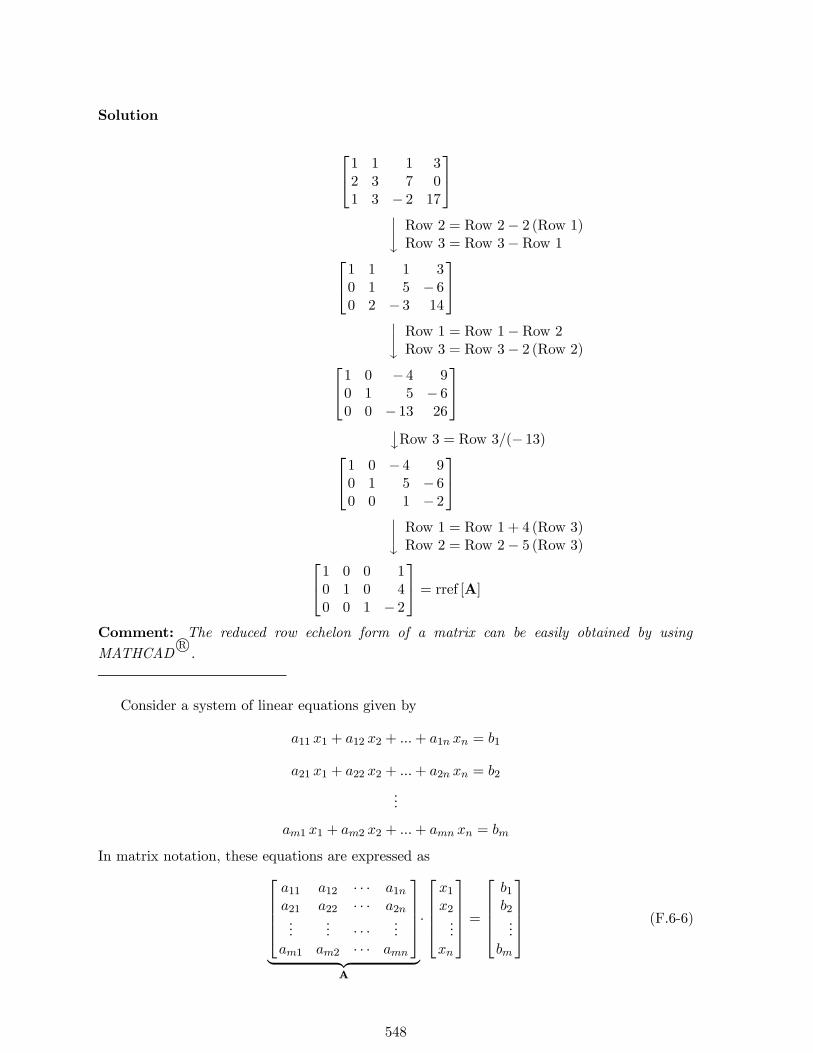
Solution

⎡⎣1 1 1 32 3 7 01 3 − 2 17

⎤⎦⏐⏐⏐y Row 2 = Row 2− 2 (Row 1)Row 3 = Row 3−Row 1⎡⎣1 1 1 3

0 1 5 − 60 2 − 3 14

⎤⎦⏐⏐⏐y Row 1 = Row 1−Row 2Row 3 = Row 3− 2 (Row 2)⎡⎣1 0 − 4 9

0 1 5 − 60 0 − 13 26

⎤⎦⏐yRow 3 = Row 3/(− 13)⎡⎣1 0 − 4 9

0 1 5 − 60 0 1 − 2

⎤⎦⏐⏐⏐y Row 1 = Row 1 + 4 (Row 3)Row 2 = Row 2− 5 (Row 3)⎡⎣1 0 0 1

0 1 0 40 0 1 − 2

⎤⎦ = rref [A]Comment: The reduced row echelon form of a matrix can be easily obtained by using

MATHCADR°.

Consider a system of linear equations given by

a11 x1 + a12 x2 + ...+ a1n xn = b1

a21 x1 + a22 x2 + ...+ a2n xn = b2

...

am1 x1 + am2 x2 + ...+ amn xn = bm

In matrix notation, these equations are expressed as⎡⎢⎢⎢⎣a11 a12 · · · a1na21 a22 · · · a2n...

... · · ·...

am1 am2 · · · amn

⎤⎥⎥⎥⎦| {z }

A

·

⎡⎢⎢⎢⎣x1x2...

xn

⎤⎥⎥⎥⎦ =⎡⎢⎢⎢⎣

b1b2...

bm

⎤⎥⎥⎥⎦ (F.6-6)

548

where A represents the coefficient matrix. The augmented matrix is a coefficient matrix havingan extra column containing the constant terms and this extra column is separated by a verticalline, i.e.,

[A |b ] =

⎡⎢⎢⎢⎣a11 a12 · · · a1na21 a22 · · · a2n...

... · · ·...

am1 am2 · · · amn

¯̄̄̄¯̄̄̄¯

b1b2...

bm

⎤⎥⎥⎥⎦ (F.6-7)

Once the augmented matrix [A |b ] can be transformed to the matrix in reduced row echelonform [C |d ] by elementary row operations, i.e.,

rrefn[A |b ]

o= [C |d ] =

⎡⎢⎢⎢⎣c11 c12 · · · c1nc21 c22 · · · c2n...

... · · ·...

cm1 cm2 · · · cmn

¯̄̄̄¯̄̄̄¯

d1d2...

dm

⎤⎥⎥⎥⎦ (F.6-8)

then, the solutions for the linear system corresponding to [C |d ] is exactly the same as the onecorresponding to [A |b ]. In other words,⎡⎢⎢⎢⎣

c11 c12 · · · c1nc21 c22 · · · c2n...

... · · ·...

cm1 cm2 · · · cmn

⎤⎥⎥⎥⎦ ·⎡⎢⎢⎢⎣x1x2...

xn

⎤⎥⎥⎥⎦ =⎡⎢⎢⎢⎣

d1d2...

dm

⎤⎥⎥⎥⎦ (F.6-9)

Example F.11 Solve the system of algebraic equations given in Example F.6.

Solution

In matrix notation, the given equations are expressed as⎡⎢⎢⎣1 1 1 12 1 − 4 13 − 1 2 22 − 3 − 1 − 3

⎤⎥⎥⎦| {z }

A

⎡⎢⎢⎣xyzw

⎤⎥⎥⎦ =⎡⎢⎢⎣

7− 15

− 34

⎤⎥⎥⎦ (1)

The augmented matrix, i.e. [A |b ], is given by

[A |b ] =

⎡⎢⎢⎣1 1 1 12 1 − 4 13 − 1 2 22 − 3 − 1 − 3

¯̄̄̄¯̄̄̄ 7− 15

− 34

⎤⎥⎥⎦ (2)

The reduced row echelon form (rref) of the augmented matrix, i.e. [C |d ], is given by

[C |d ] =

⎡⎢⎢⎣1 0 0 00 1 0 00 0 1 00 0 0 1

¯̄̄̄¯̄̄̄ − 32

17

⎤⎥⎥⎦ (3)

549

Since the linear system corresponding to [C |d ] is exactly the same as the one corresponding to[A |b ], then ⎡⎢⎢⎣

1 0 0 00 1 0 00 0 1 00 0 0 1

⎤⎥⎥⎦⎡⎢⎢⎣xyzw

⎤⎥⎥⎦ =⎡⎢⎢⎣− 3217

⎤⎥⎥⎦ (4)

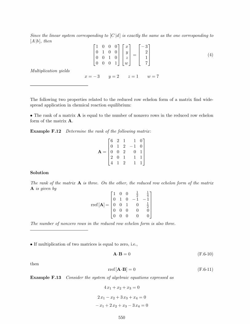
Multiplication yieldsx = − 3 y = 2 z = 1 w = 7

The following two properties related to the reduced row echelon form of a matrix find wide-spread application in chemical reaction equilibrium:

• The rank of a matrix A is equal to the number of nonzero rows in the reduced row echelonform of the matrix A.

Example F.12 Determine the rank of the following matrix :

A =

⎡⎢⎢⎢⎢⎣6 2 1 1 00 1 2 − 1 00 0 2 0 12 0 1 1 14 1 2 1 1

⎤⎥⎥⎥⎥⎦Solution

The rank of the matrix A is three. On the other, the reduced row echelon form of the matrixA is given by

rref [A] =

⎡⎢⎢⎢⎢⎣1 0 0 1

214

0 1 0 − 1 − 10 0 1 0 1

20 0 0 0 00 0 0 0 0

⎤⎥⎥⎥⎥⎦The number of nonzero rows in the reduced row echelon form is also three.

• If multiplication of two matrices is equal to zero, i.e.,

A·B = 0 (F.6-10)

thenrref [A·B] = 0 (F.6-11)

Example F.13 Consider the system of algebraic equations expressed as

4x1 + x2 + x3 = 0

2x1 − x2 + 3x3 + x4 = 0

−x1 + 2x2 + x3 − 3x4 = 0

550

In matrix notation, the given equations are written as

⎡⎣ 4 1 1 02 − 1 3 1− 1 2 1 − 3

⎤⎦| {z }

A

·

⎡⎢⎢⎣x1x2x3x4

⎤⎥⎥⎦ =⎡⎣000

⎤⎦ (1)

The reduced row echelon form of the matrix A is

rref [A] =

⎡⎢⎢⎣1 0 0 − 3

2

0 1 0 72

0 0 1 52

⎤⎥⎥⎦ (2)

Therefore, Eq. (F.6-11) is written as⎡⎢⎢⎣1 0 0 − 3

2

0 1 0 72

0 0 1 52

⎤⎥⎥⎦ ·⎡⎢⎢⎣x1x2x3x4

⎤⎥⎥⎦ =⎡⎣000

⎤⎦ (3)

or, the given set of equations are expressed as

x1 −3

2x4 = 0

x2 +7

2x4 = 0

x3 +5

2x4 = 0

551

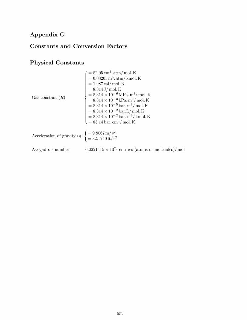
Appendix G

Constants and Conversion Factors

Physical Constants

Gas constant (R)

⎧⎪⎪⎪⎪⎪⎪⎪⎪⎪⎪⎪⎪⎪⎪⎨⎪⎪⎪⎪⎪⎪⎪⎪⎪⎪⎪⎪⎪⎪⎩

= 82.05 cm3. atm/mol.K= 0.08205m3. atm/ kmol.K= 1.987 cal/mol.K= 8.314 J/mol.K= 8.314× 10− 6MPa.m3/mol.K= 8.314× 10− 3 kPa.m3/mol.K= 8.314× 10− 5 bar.m3/mol.K= 8.314× 10− 2 bar.L/mol.K= 8.314× 10− 2 bar.m3/ kmol.K= 83.14 bar. cm3/mol.K

Acceleration of gravity (g)½= 9.8067m/ s2

= 32.1740 ft/ s2

Avogadro’s number 6.0221415× 1023 entities (atoms or molecules)/mol

552

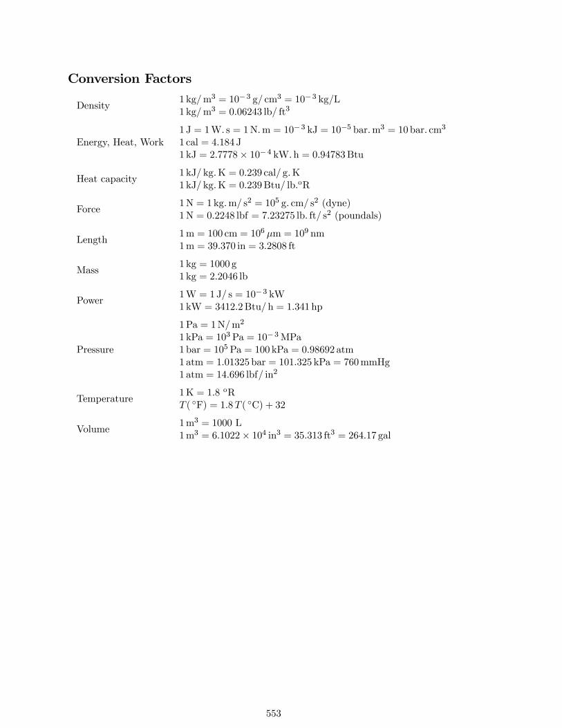
Conversion Factors

Density1 kg/m3 = 10− 3 g/ cm3 = 10− 3 kg/L1 kg/m3 = 0.06243 lb/ ft3

Energy, Heat, Work1 J = 1W. s = 1N.m = 10− 3 kJ = 10−5 bar.m3 = 10bar. cm3

1 cal = 4.184 J1 kJ = 2.7778× 10− 4 kW.h = 0.94783Btu

Heat capacity1 kJ/ kg.K = 0.239 cal/ g.K1kJ/ kg.K = 0.239Btu/ lb.oR

Force1N = 1kg.m/ s2 = 105 g. cm/ s2 (dyne)1N = 0.2248 lbf = 7.23275 lb. ft/ s2 (poundals)

Length1m = 100 cm = 106 μm = 109 nm1m = 39.370 in = 3.2808 ft

Mass1 kg = 1000 g1 kg = 2.2046 lb

Power1W = 1J/ s = 10− 3 kW1kW = 3412.2Btu/h = 1.341 hp

Pressure

1Pa = 1N/m2

1 kPa = 103 Pa = 10− 3MPa1bar = 105 Pa = 100 kPa = 0.98692 atm1 atm = 1.01325 bar = 101.325 kPa = 760mmHg1 atm = 14.696 lbf/ in2

Temperature1K = 1.8 oRT ( ◦F) = 1.8T ( ◦C) + 32

Volume1m3 = 1000 L1m3 = 6.1022× 104 in3 = 35.313 ft3 = 264.17 gal

553

Appendix H

Databanks, Simulation Programs, Books, Websites

Finding thermochemical data and selecting proper thermodynamic model are major challenges,among others, in the design of a chemical plant. Some of the commercial and/or free-to-useliterature on the subject are provided below.

DATABANKS

1. CODATA (The Committee on Data for Science and Technology)

• http://www.codata.org/resources/databases/key1.html

• It provides internationally agreed values for the thermodynamic properties of key chemicalsubstances.

2. DETHERM

• http://i-systems.dechema.de/detherm

• It provides thermophysical properties of pure substances and mixtures for design andoptimization of chemical plants and apparatus.

3. DIPPR (Design Institute for Physical Properties)

• http://dippr.byu.edu/student.asp

• Student version of the database provides students to access 100 compounds.

4. Dortmund Data Bank Software Package (DDBSP)

• http://www.ddbst.de

• It provides thermodynamic and transport properties of pure components and mixturesfor use in process design and development as well as special programs for data correlation,estimation and process synthesis.

5. FactSage

• http://factsage.com

• It is an integrated datebase computing system in chemical thermodynamics.

6. Kaye and Laby Online

• http://www.kayelaby.npl.co.uk

• It provides tables of physical and chemical constants.

554

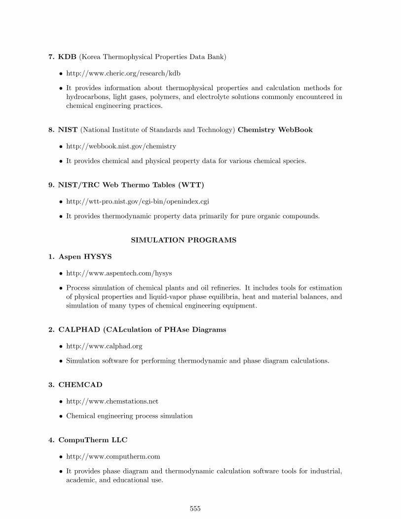
7. KDB (Korea Thermophysical Properties Data Bank)

• http://www.cheric.org/research/kdb

• It provides information about thermophysical properties and calculation methods forhydrocarbons, light gases, polymers, and electrolyte solutions commonly encountered inchemical engineering practices.

8. NIST (National Institute of Standards and Technology) Chemistry WebBook

• http://webbook.nist.gov/chemistry

• It provides chemical and physical property data for various chemical species.

9. NIST/TRC Web Thermo Tables (WTT)

• http://wtt-pro.nist.gov/cgi-bin/openindex.cgi

• It provides thermodynamic property data primarily for pure organic compounds.

SIMULATION PROGRAMS

1. Aspen HYSYS

• http://www.aspentech.com/hysys

• Process simulation of chemical plants and oil refineries. It includes tools for estimationof physical properties and liquid-vapor phase equilibria, heat and material balances, andsimulation of many types of chemical engineering equipment.

2. CALPHAD (CALculation of PHAse Diagrams

• http://www.calphad.org

• Simulation software for performing thermodynamic and phase diagram calculations.

3. CHEMCAD

• http://www.chemstations.net

• Chemical engineering process simulation

4. CompuTherm LLC

• http://www.computherm.com

• It provides phase diagram and thermodynamic calculation software tools for industrial,academic, and educational use.

555

5. EQS4WIN (Chemical EQuilibrium Software 4WINdows)

• http://www.mathtrek.com

• Calculates equilibrium compositions for reacting systyems.

6. MTDATA

• http://www.npl.co.uk/advanced-materials/measurement-techniques/modelling/mtdata

• Software tool for the calculation of phase equilibria and thermodynamic properties.

7. Physical Property Data Service (PPDS)

• http://www.tuvnel.com/contents/PPDS.aspx

• It provides key information on more than 15000 chemicals, constant and variable physicalproperties, thermodynamic model sets, and flash calculations.

8. PRODE

• http://www.prode.com

• Solves phase equilibrium separations, prints phase envelopes and phase diagrams, calcu-lates temperature or pressure at dew point, bubble point or specified liquid fraction.

9. ProSim

• http://www.prosim.net

• Process simulation and optimization for design and operation of industrial processes.

10. Thermo-Calc

• http://www.thermocalc.com

• Simulation software for performing thermodynamic calculations.

11. WinSim

• http://www.winsim.com

• Process simulation for chemical and hydrocarbon processes including refining, refrigera-tion, petrochemical, gas processing, gas treating, pipelines, fuel cells, ammonia, methanol,sulfur and hydrogen facilities.

NOTE: It is extremely important to keep in mind that the values obtained from simulationpackages do not guarantee correct results. One should understand the thermodynamic assump-tions on which the simulation program is based on. For more details on the subject the readermay refer to:

• Agarwal, R., Y.K. Li, O. Santollani, M.A. Satyro and A. Vieler, 2001, "Uncovering therealities of simulation - Part 1", Chemical Engineering Progress 97 (5), 42-52.

• Agarwal, R., Y.K. Li, O. Santollani, M.A. Satyro and A. Vieler, 2001, "Uncovering therealities of simulation - Part 2", Chemical Engineering Progress 97 (6), 64-72.

556

BOOKS

1. Assael, M.J., J.P.M. Trusler, T.F. Tsolakis, Thermophysical Properties of Fluids: An Intro-duction to Their Prediction, Imperial College Press, 1996.

2. Barin, I., Thermophysical Data of Pure Substances, VCH, Weinhem, 1989.

3. DECHEMA - Chemistry Data Series

Vol.I Vapor-Liquid Equilibrium Data CollectionVol. II Critical Data of Pure SubstancesVol. III Heats of Mixing Data CollectionVol .IV Recommended Data of Selected Compounds and Binary MixturesVol. V Liquid-Liquid Equilibrium Data CollectionVol. VI Vapor-Liquid Equilibria for Mixtures of Low Boiling SubstancesVol. VIII Solid-Liquid Equilibrium Data CollectionVol. IX Activity Coefficients at Infinite DilutionVol. X Thermal Conductivity and Viscosity Data of Fluid MixturesVol. XII Electrolyte Data CollectionVol. XIV Polymer Solution Data CollectionVol. XV Solubility and Related Properties of Large Complex Chemicals

4. Millat, J., J.H. Dymond, C.A. Nieto de Castro, Transport Properties of Fluids, CambridgeUniversity Press, 1996.

5. NIST-JANAF Thermochemical Tables, 4th Ed., Chase, M.W. Jr. (Ed.), Springer, 1998.

6. Poling, B.E., J.M. Prausnitz, J.P. O’Connell, The Properties of Gases and Liquids, 5th Ed.,McGraw-Hill, New York, 2001.

7. TRC Thermodynamic Tables - Hydrocarbons, Ed. Frenkel, M., NIST, Boulder, CO, Stan-dard Reference Data Program, Publication Series NSRDS-NIST-75 (1942-2007), Gaithersburg,MD.

8. TRC Thermodynamic Tables - Non-Hydrocarbons, Ed. Frenkel, M., NIST, Boulder, CO,Standard Reference Data Program, Publication Series NSRDS-NIST-74 (1955-2007), Gaithers-burg, MD.

9. Vargaftik, N.B., Y.K. Vinogradov, V.S. Yargin, Handbook of Physical Properties of Liquidsand Gases, Third Augmented and Revised Ed., Begell House, New York, 1996.

10. Yaws, C.L., Thermodynamic and Physical Property Data, Gulf Pub. Company, Houston,Texas, 1992.

557

WEBSITES

1. Chemical Reaction Stoichiometry (CRS)hhtp://www.chemical-stoichiometry.net

2. Gibbs Modelshttp://www.iastate.edu/~jolls

3. Macatea Productions - Thermo Workshophttp://www.macatea.com/wshop

4. Nano, Quantum & Statistical Mechanics & Thermodynamics Educational Siteshttp://tigger.uic.edu/~mansoori/Thermodynamics.Educational.Sites_html

5. Thermographicshttp://www.owlnet.rice.edu/~wgchap/Phase/v3dcmnt.htm

558

Appendix

Documents

Transcript of Appendix