Analysis on Energy Consumption of Road Transportation in China

Jian Chai, Quanying Lu, Xiaoyang Zhou

OUTLINE

INTRODUCTIONI.

II. LITERATURE REVIEW

SAMPLING APPROACH

MODELING APPROACH AND DATA ANALYSIS

CONCLUSIONS

III.

IV.

V

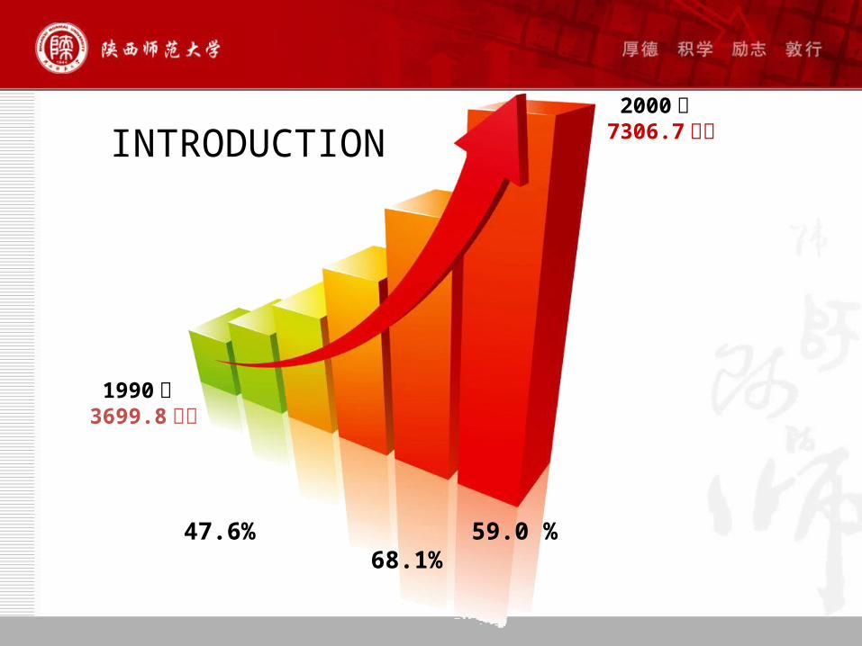
1990 年 3699.8 万吨

2000 年 7306.7 万吨INTRODUCTION

47.6% 59.0 % 68.1%

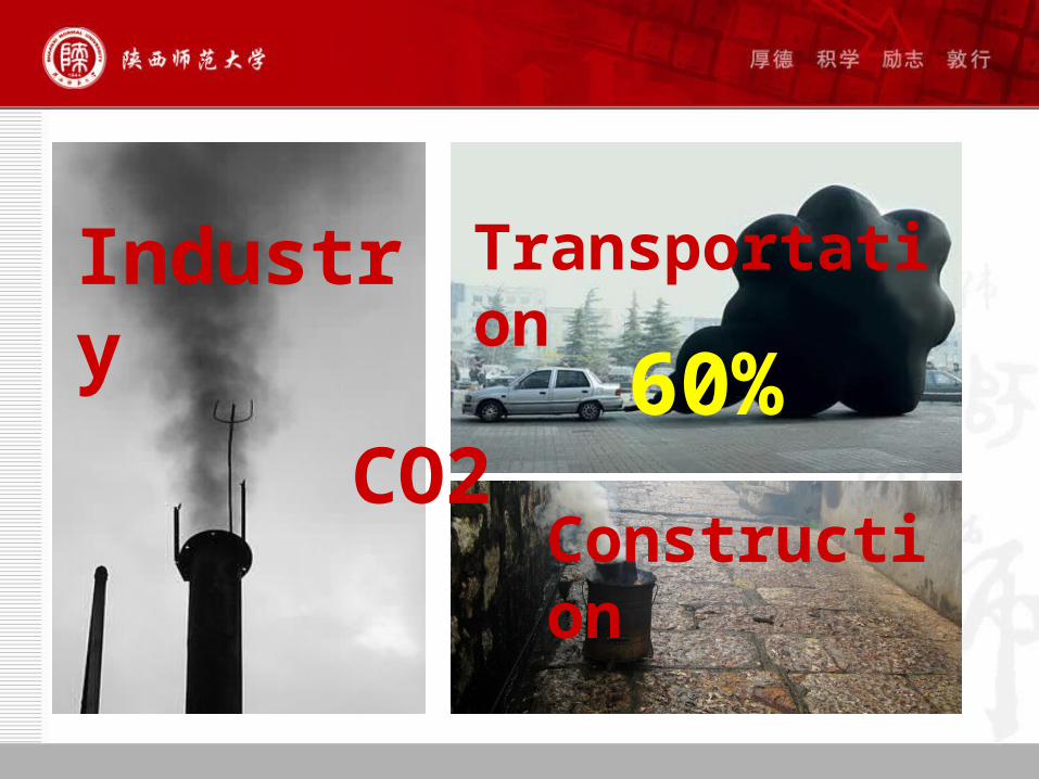
TransportationIndustry

ConstructionCO2

60%

Two main difficulties in Transportation Research

• China's transport sector statistics is not careful, the departments of carbon dioxide output many estimated using mode, there is no accurate statistical results.

• Strategy of modeling 

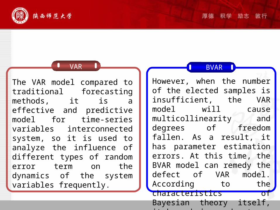
VAR BVAR

The VAR model compared to traditional forecasting methods, it is a effective and predictive model for time-series variables interconnected system, so it is used to analyze the influence of different types of random error term on the dynamics of the system variables frequently.

However, when the number of the elected samples is insufficient, the VAR model will cause multicollinearity and degrees of freedom fallen. As a result, it has parameter estimation errors. At this time, the BVAR model can remedy the defect of VAR model. According to the characteristics of Bayesian theory itself, it has obvious advantages in the case of small samples.

Using different prior information on the VAR model of posterior distribution effect is relatively rare. Posterior mean can be considered some suitable loss function. The loss function is minimized using commonly used in the BVAR model of the article a few.

Shawn Ni, Dongchu Sun (2003) discussed different loss functions common information without prior different and several under, VAR model estimation results, and the use of U.S. macroeconomic data to illustrate. The results show that, in the constant prior distribution, LINEX estimation of loss function slightly than the estimation results obtained under the square loss function, the difference of the point, but the general case of LINEX loss better.

IPCC Mobile sources (Department of transportation)

 carbon dioxide emissions accounting methods

• The top-down method• The down to top method

n

i ii

C EF k

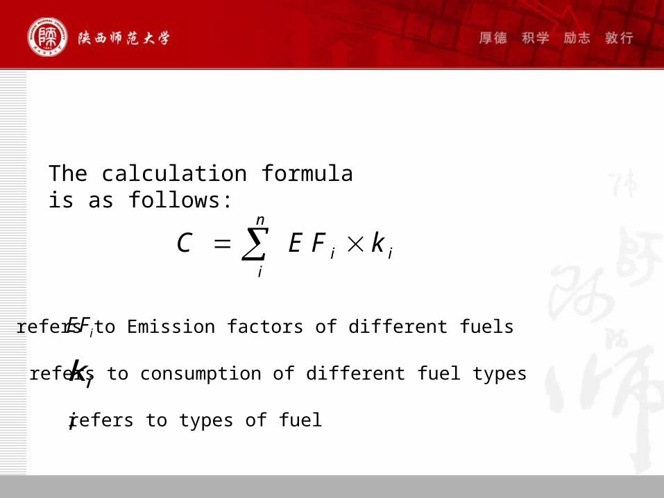
The calculation formula is as follows:

iEF

ik

i

refers to Emission factors of different fuels

refers to consumption of different fuel types

refers to types of fuel

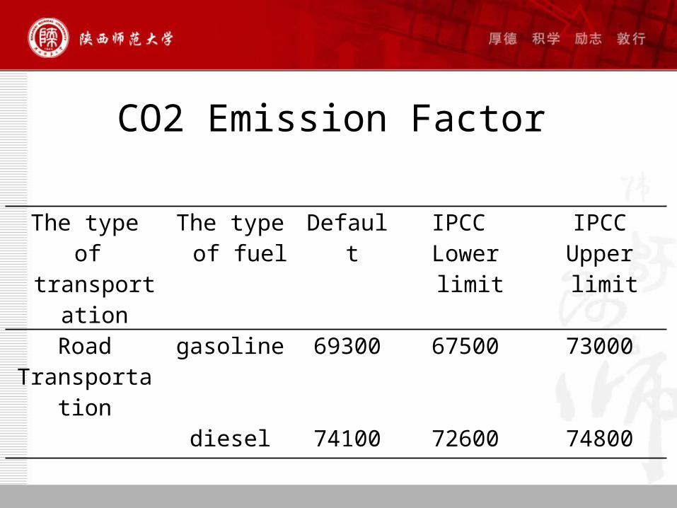
CO2 Emission Factor

The type of transportation

The type of fuel

Default IPCC Lower limit

IPCCUpper limit

Road Transportation

gasoline 69300 67500 73000

diesel 74100 72600 74800

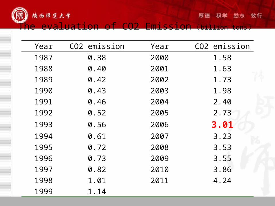
The evaluation of CO2 Emission （ billion tons）Year CO2 emission Year CO2 emission

1987 0.38 2000 1.58

1988 0.40 2001 1.63

1989 0.42 2002 1.73

1990 0.43 2003 1.98

1991 0.46 2004 2.40

1992 0.52 2005 2.73

1993 0.56 2006 3.011994 0.61 2007 3.23

1995 0.72 2008 3.53

1996 0.73 2009 3.55

1997 0.82 2010 3.86

1998 1.01 2011 4.24

1999 1.14

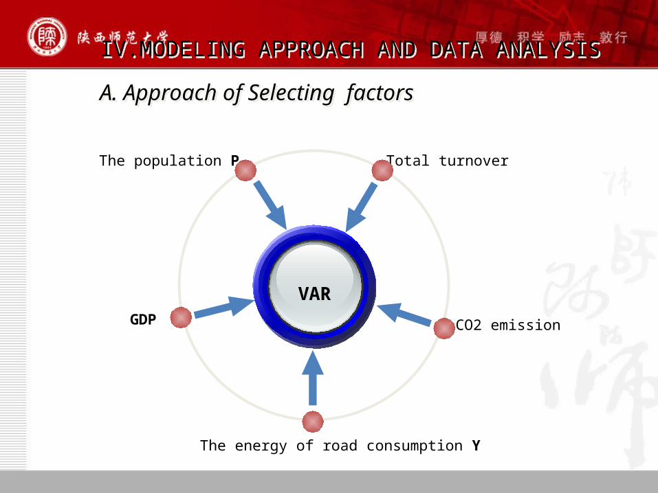
Total turnoverThe population P

The energy of road consumption Y

GDP

VAR

A. Approach of Selecting factorsA. Approach of Selecting factors

CO2 emission

IV.MODELING APPROACH AND DATA ANALYSISIV.MODELING APPROACH AND DATA ANALYSIS

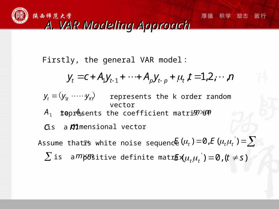
Firstly, the general VAR model：

A. VAR Modeling ApproachA. VAR Modeling Approach

1 1 , 1, 2, ,t t p t p ty c A y A y t n

represents the k order random vector1t t Kty y y （ ）

1A pA m m to represents the coefficient matrix of

c is a m dimensional vector

Assume that t is white noise sequence'( ) 0, ( )t t tE E

is a m m positive definite matrix '( ) 0, ( )t tE t s

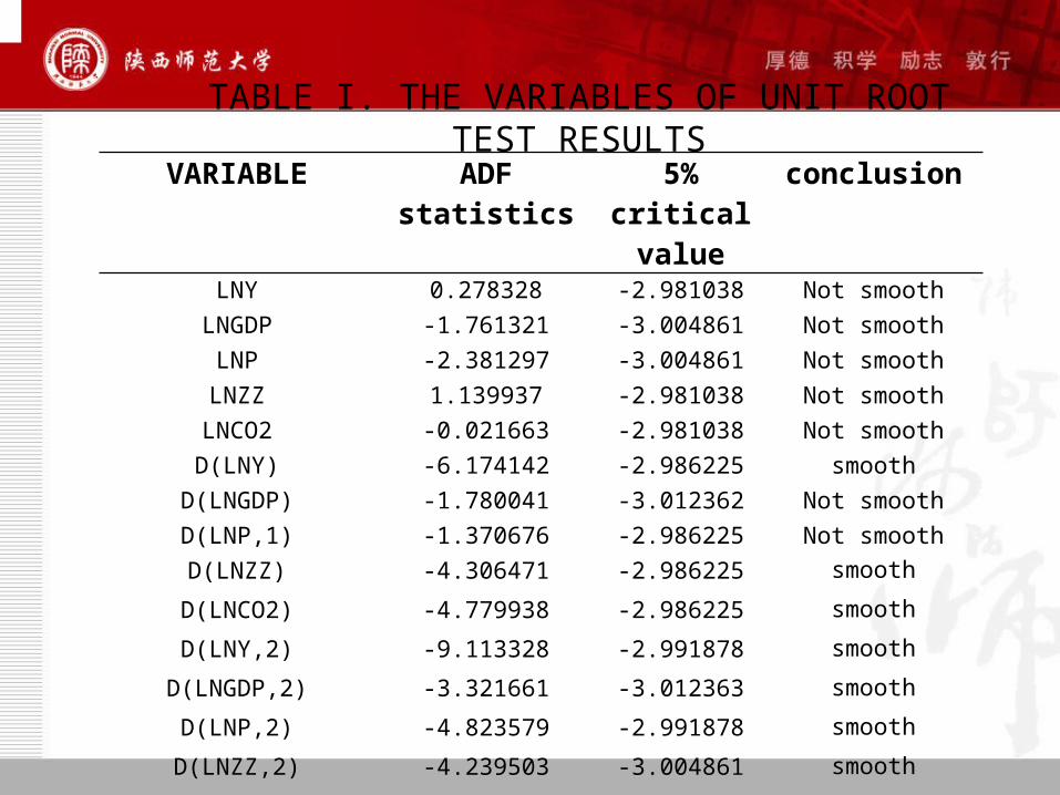
TABLE I. THE VARIABLES OF UNIT ROOT TEST RESULTSVARIABLE ADF statistics 5% critical

valueconclusion

LNY 0.278328 -2.981038 Not smooth

LNGDP -1.761321 -3.004861 Not smooth

LNP -2.381297 -3.004861 Not smooth

LNZZ 1.139937 -2.981038 Not smooth

LNCO2 -0.021663 -2.981038 Not smooth

D(LNY) -6.174142 -2.986225 smooth

D(LNGDP) -1.780041 -3.012362 Not smooth

D(LNP,1) -1.370676 -2.986225 Not smooth

D(LNZZ) -4.306471 -2.986225 smooth

D(LNCO2) -4.779938 -2.986225 smooth

D(LNY,2) -9.113328 -2.991878 smooth

D(LNGDP,2) -3.321661 -3.012363 smooth

D(LNP,2) -4.823579 -2.991878 smooth

D(LNZZ,2) -4.239503 -3.004861 smooth

D(LNCO2,2) -5.684127 -2.998064 smooth

LNP

LNY

LNGDP

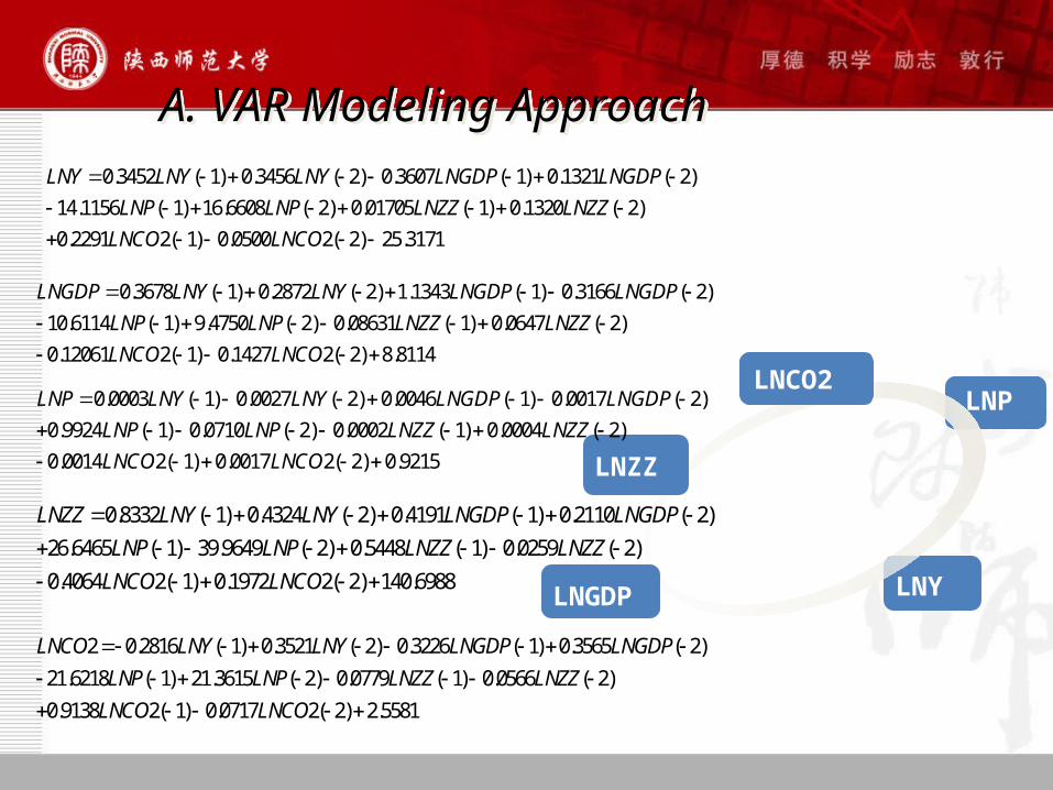
A. VAR Modeling ApproachA. VAR Modeling Approach

LNGDP

VAR

0.3452 ( 1) 0.3456 ( 2) 0.3607 ( 1) 0.1321 ( 2)

14.1156 ( 1) 16.6608 ( 2) 0.01705 ( 1) 0.1320 ( 2)

0.2291 2( 1) 0.0500 2( 2) 25.3171

LNY LNY LNY LNGDP LNGDP

LNP LNP LNZZ LNZZ

LNCO LNCO

LNZZ

LNY

LNCO2

0.3678 ( 1) 0.2872 ( 2) 1.1343 ( 1) 0.3166 ( 2)

10.6114 ( 1) 9.4750 ( 2) 0.08631 ( 1) 0.0647 ( 2)

0.12061 2( 1) 0.1427 2( 2) 8.8114

LNGDP LNY LNY LNGDP LNGDP

LNP LNP LNZZ LNZZ

LNCO LNCO

0.0003 ( 1) 0.0027 ( 2) 0.0046 ( 1) 0.0017 ( 2)

0.9924 ( 1) 0.0710 ( 2) 0.0002 ( 1) 0.0004 ( 2)

0.0014 2( 1) 0.0017 2( 2) 0.9215

LNP LNY LNY LNGDP LNGDP

LNP LNP LNZZ LNZZ

LNCO LNCO

0.8332 ( 1) 0.4324 ( 2) 0.4191 ( 1) 0.2110 ( 2)

26.6465 ( 1) 39.9649 ( 2) 0.5448 ( 1) 0.0259 ( 2)

0.4064 2( 1) 0.1972 2( 2) 140.6988

LNZZ LNY LNY LNGDP LNGDP

LNP LNP LNZZ LNZZ

LNCO LNCO

2 0.2816 ( 1) 0.3521 ( 2) 0.3226 ( 1) 0.3565 ( 2)

21.6218 ( 1) 21.3615 ( 2) 0.0779 ( 1) 0.0566 ( 2)

0.9138 2( 1) 0.0717 2( 2) 2.5581

LNCO LNY LNY LNGDP LNGDP

LNP LNP LNZZ LNZZ

LNCO LNCO

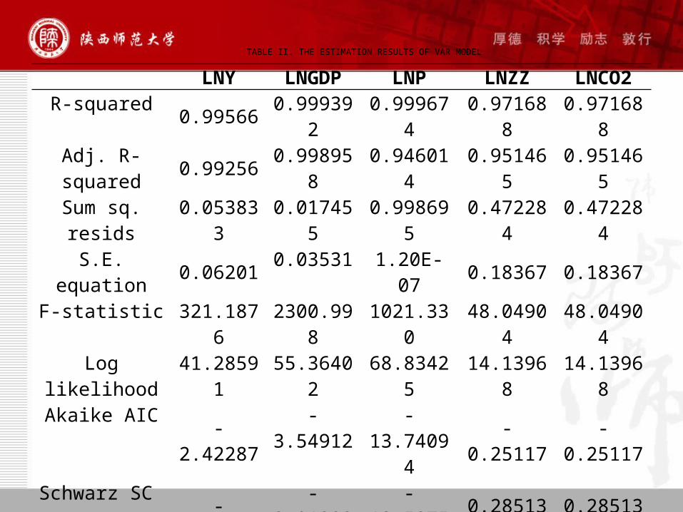
TABLE II. THE ESTIMATION RESULTS OF VAR MODEL

LNY LNGDP LNP LNZZ LNCO2R-squared 0.99566 0.999392 0.999674 0.971688 0.971688

Adj. R-squared 0.99256 0.998958 0.946014 0.951465 0.951465Sum sq. resids 0.053833 0.017455 0.998695 0.472284 0.472284S.E. equation 0.06201 0.03531 1.20E-07 0.18367 0.18367

F-statistic 321.1876 2300.998 1021.330 48.04904 48.04904Log likelihood 41.28591 55.36402 68.83425 14.13968 14.13968

Akaike AIC -2.42287 -3.54912 -13.74094 -0.25117 -0.25117Schwarz SC -1.88657 -3.01282 -13.58755 0.285131 0.285131

Mean dependent 10.82368 11.32511 17.42617 11.27772 11.27772S.D. dependent 0.718915 1.093659 0.006776 0.833702 0.833702

 Determinant resid covariance (dof adj.)

1.42E-17

 Determinant resid covariance  7.83E-19 Log likelihood 343.7734 Akaike information criterion -23.1019 Schwarz criterion -20.4204

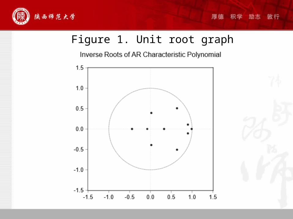
Figure 1. Unit root graph

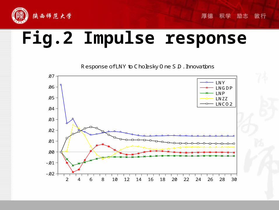
Fig.2 Impulse response

-.02

-.01

.00

.01

.02

.03

.04

.05

.06

.07

2 4 6 8 10 12 14 16 18 20 22 24 26 28 30

LNYLNGDPLNPLNZZLNCO2

Response of LNY to Cholesky One S.D. Innovations

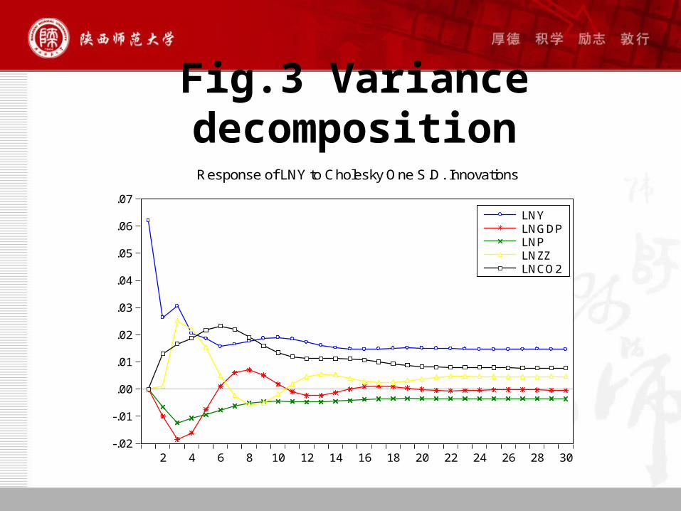
Fig.3 Variance decomposition

-.02

-.01

.00

.01

.02

.03

.04

.05

.06

.07

2 4 6 8 10 12 14 16 18 20 22 24 26 28 30

LNYLNGDPLNPLNZZLNCO2

Response of LNY to Cholesky One S.D. Innovations

B. BVAR Modeling Approach

Although the VAR model does not consider the economic theory model has improved, but because of the VAR model does not consider the economic theory, it cannot give any structural interpretation, which makes people to question this way. Secondly, the main shortcomings of VAR model are quite a few parameters need to estimate, the data sample sequence length requirement is too large. When the sample size is small, the parameter estimator error is bigger. But the Bias theory has the absolute advantage in the case of small samples, provides a new method for estimating the parameters of VAR model solves the problem of excessive. So this paper uses VAR and BVAR model respectively on the Shaanxi province coal consumption market analysis, and then comparing the predicted results of two models.

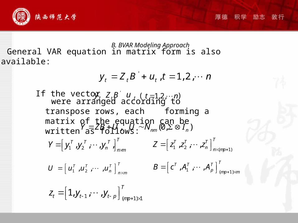
B. BVAR Modeling ApproachGeneral VAR equation in matrix form is also

available:' , 1, 2,t t ty Z B u t n

If the vectorty '

tZ B tu 1,2,t n ( )

were arranged according to transpose rows, each forming a matrix of the equation can be written as follows: , (0, )nm nY ZB U U N I

1 2, , , ,TT T T

n n mY y y y

1 2 ( 1)

, , ,TT T T

n n mpZ z z z

1 2, , ,TT T T

n n mU u u u

1 ( 1)

, , ,TT T T

p mp mB c A A

1 ( 1) 11, , ,

T

t t t p mpz y y

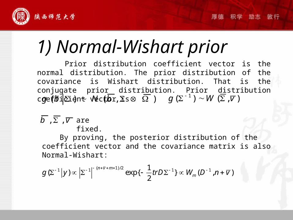
1) Normal-Wishart prior Prior distribution coefficient vector is the normal distribution. The prior distribution of the covariance is Wishart distribution. That is the conjugate prior distribution. Prior distribution coefficient vector is

( ) ( , )g b N b 1( ) ( , )g W v

, ,b v are fixed.

By proving, the posterior distribution of the coefficient vector and the covariance matrix is also Normal-Wishart:

( 1)/21 1 1 11( ) exp{ } ( , )

2

n v m

mg y trD W D n v

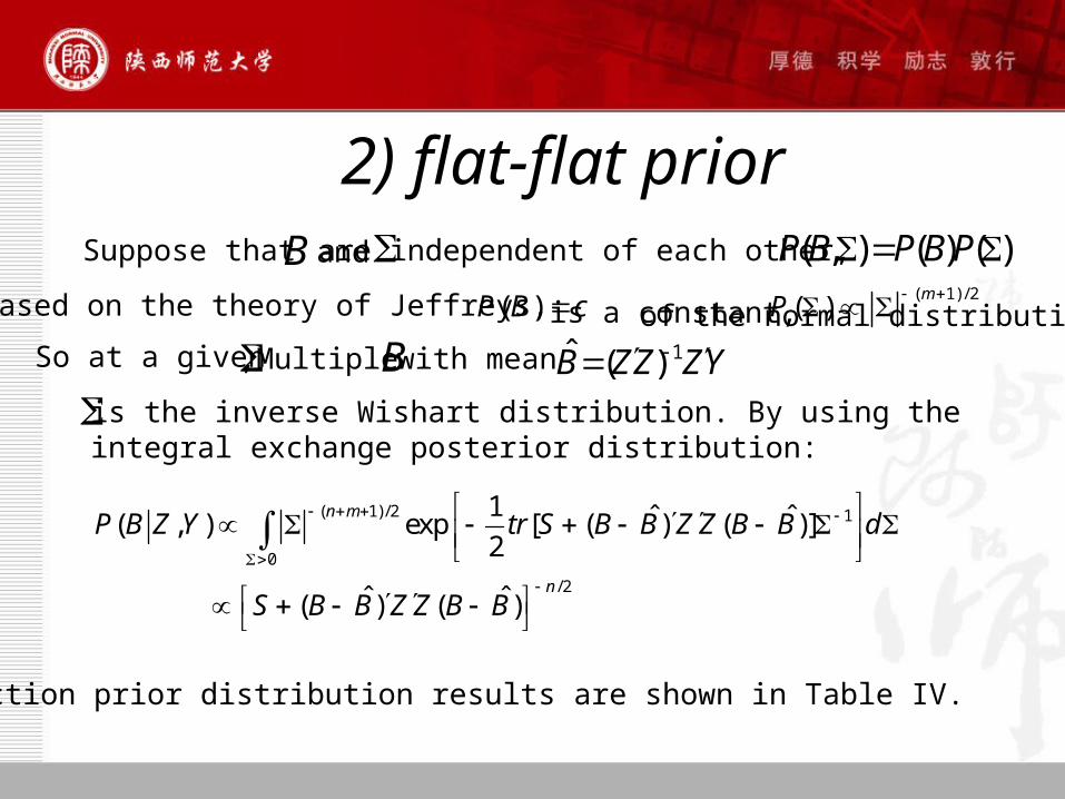
2) flat-flat priorSuppose that B and are independent of each other, ( , ) ( ) ( )P B P B P

Based on the theory of Jeffreys, ( )P B c is a constant, ( 1)/2

( )m

P

So at a given ,Multiple with mean B 1ˆ ( )B Z Z Z Y of the normal distribution,

is the inverse Wishart distribution. By using the integral exchange posterior distribution:

( 1)/2 1

0

/2

1 ˆ ˆ( , ) exp [ ( ) ( )]2

ˆ ˆ( ) ( )

n m

n

P B Z Y tr S B B Z Z B B d

S B B Z Z B B

prediction prior distribution results are shown in Table IV.

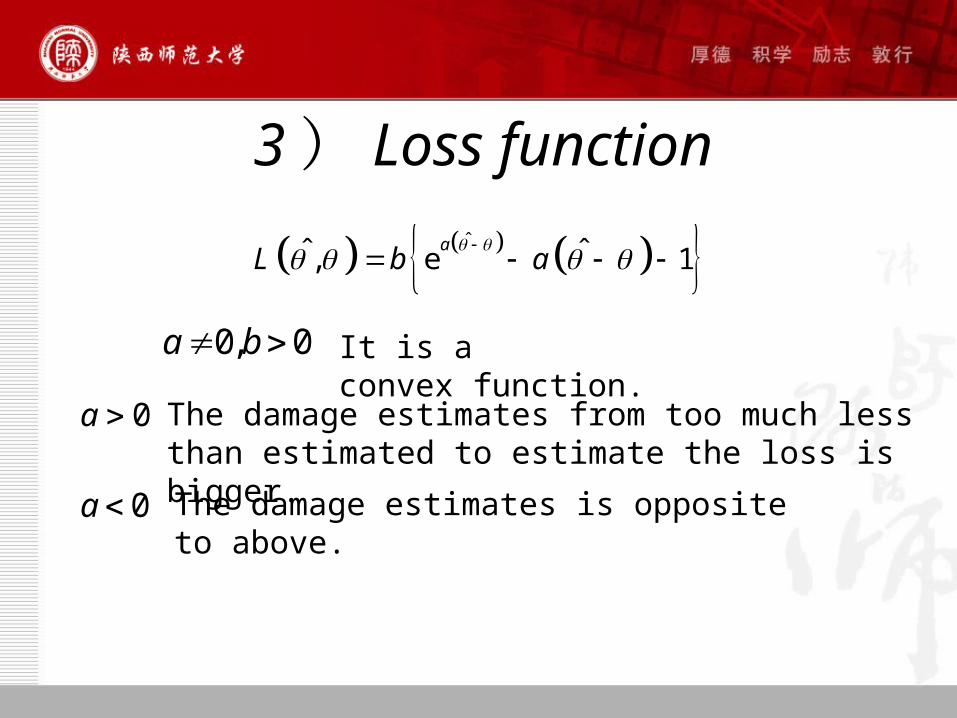
3） Loss function

ˆˆ ˆ, e 1a

L b a

0, 0a b

0a

It is a convex function.

The damage estimates from too much less than estimated to estimate the loss is bigger.

0a The damage estimates is opposite to above.

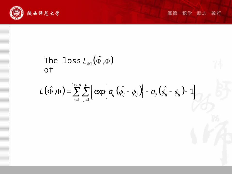
1

1 1

ˆ ˆˆ , exp 1Lp p

ij ij ij ij ij iji j

L a a

1ˆ ,L The loss of

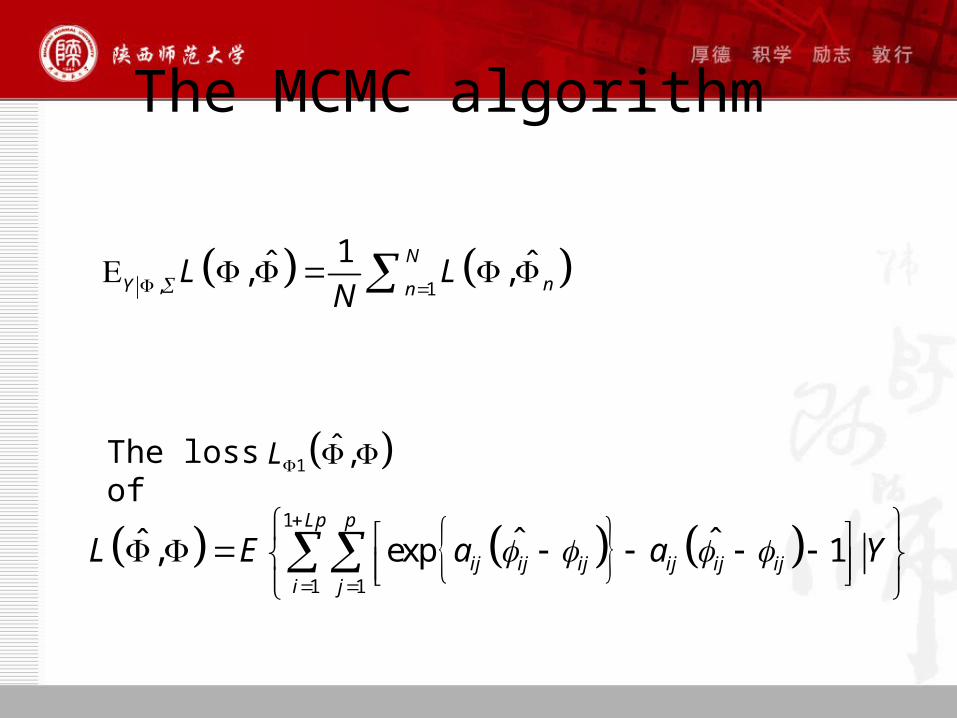
The MCMC algorithm

1

1 1

ˆ ˆˆ , exp 1Lp p

ij ij ij ij ij iji j

L E a a Y

1ˆ ,L The loss of

, 1

1ˆ ˆ, ,N

nY nL L

N

We let the parameter corresponding to the intercept term 1 j be 0.001.

implying a near symmetric loss, and that corresponding to non-intercept term be -4. The value -4 was used by Zellner (1986) for estimating the normal means.

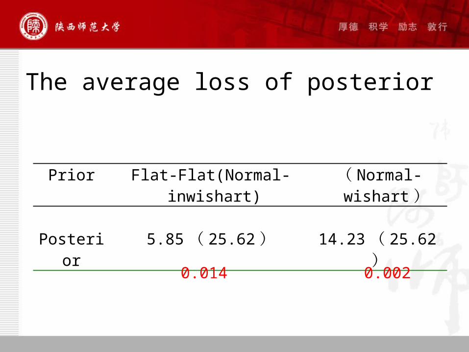
Prior Flat-Flat(Normal-inwishart) （ Normal-

wishart）

Posterior 5.85（ 25.62） 14.23（ 25.62）

The average loss of posterior

0.014 0.002

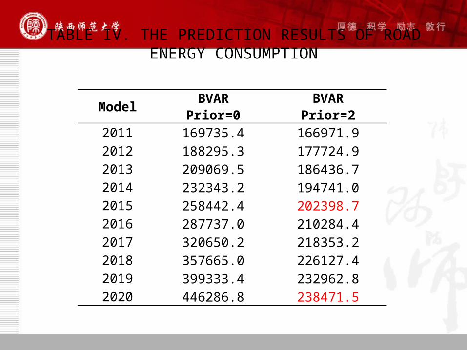
TABLE IV. THE PREDICTION RESULTS OF ROAD ENERGY CONSUMPTION

Model BVARPrior=0

BVARPrior=2

2011 169735.4 166971.92012 188295.3 177724.92013 209069.5 186436.72014 232343.2 194741.02015 258442.4 202398.72016 287737.0 210284.42017 320650.2 218353.22018 357665.0 226127.42019 399333.4 232962.82020 446286.8 238471.5

V.CONCLUSIONSWhen we assumed a positive impact of GDP, road energy consumption reaches a nadir in the third period, then declines gradually and then begins to converge in the 20th period, indicating that the GDP impact on gas consumption is significant from the third year onwards and lasts for a long period. When positive impact of population growth rate is assumed, road energy consumption can be seen to be declining gradually before the 2th period and then begins to increase steadily until convergence in the 9th period. However, a decline in population growth has a negative impact on road energy consumption. When a positive impact of total turnover is assumed, road energy consumption reaches a peak in the 4th period after a period of fluctuation, and then can be seen to be declining in the 8th period, with convergence beginning in the 15th period. When a positive impact of CO2 emission is assumed, road energy consumption increasing gradually before the 6th period, and then can be seen to be declining in the 7th period, with convergence beginning in the 15th period. The result shows that if we give CO2 emission a positive impact, the impact of road energy consumption is also positive in the short term.

• The result shows that the loss is minimal under the Plat-plat prior.

• At the end of the twelfth five-year plan ( 2011-2015)， China will nearly approach 202398.7 one thousand tons of oil equivalent, in 2020, China nearly 238471.5 one thousand tons of oil equivalent.

Thank you!