ANALYSIS AND IMPROVEMENT OF MULTIPLE OPTIMAL LEARNING FACTORS FOR FEED-FORWARD NETWORKS

PRAVEEN JESUDHASGrad Student, DEPT. OF ELECTRICAL ENGINEERING

UNIVERSITY OF TEXAS AT ARLINGTON

DR. MICHAEL T MANRY, SR. MEMBER IEEE

PROFESSOR, DEPT. OF ELECTRICAL ENGINEERINGUNIVERSITY OF TEXAS AT ARLINGTON

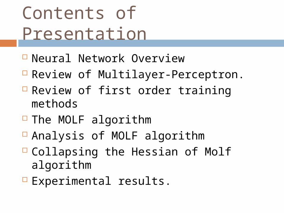
Contents of Presentation

Neural Network Overview Review of Multilayer-Perceptron. Review of first order training methods The MOLF algorithm Analysis of MOLF algorithm Collapsing the Hessian of Molf algorithm Experimental results.

Neural net overview

Input (xp)

NeuralNetworks

Output (yp)

xp - Input vector

yp - Actual output

tp - Desired output

Nv - Number of Patterns

1 x1 t1

2 x2 t2

. . . . . . Nv xNv tNv

.

Contents of a

Training File

The Multilayer Perceptron

op(k) = f(np(k))

Input Layer

Output Layer Hidden Layer

xp (1)

xp (3)

xp (2)

yp (M)

yp (3)

yp (2)

yp (1)

np (Nh) op (Nh)

np (1) op (1)W Woh

Woixp (N+1)

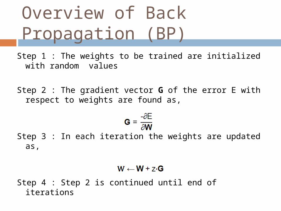
Overview of Back Propagation (BP)

Step 1 : The weights to be trained are initialized with random values

Step 2 : The gradient vector G of the error E with respect to weights are found as,

Step 3 : In each iteration the weights are updated as,

Step 4 : Step 2 is continued until end of iterations

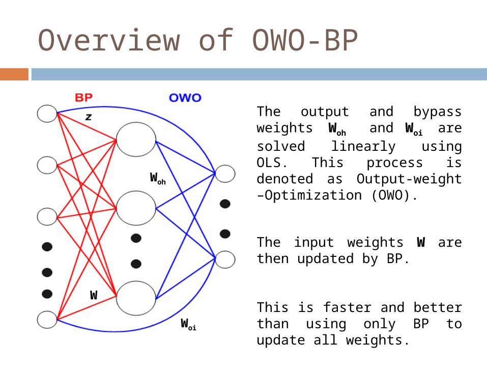
Overview of OWO-BP

The output and bypass weights Woh and Woi are solved linearly using OLS. This process is denoted as Output-weight –Optimization (OWO).

The input weights W are then updated by BP.

This is faster and better than using only BP to update all weights.

Woh

Woi

W

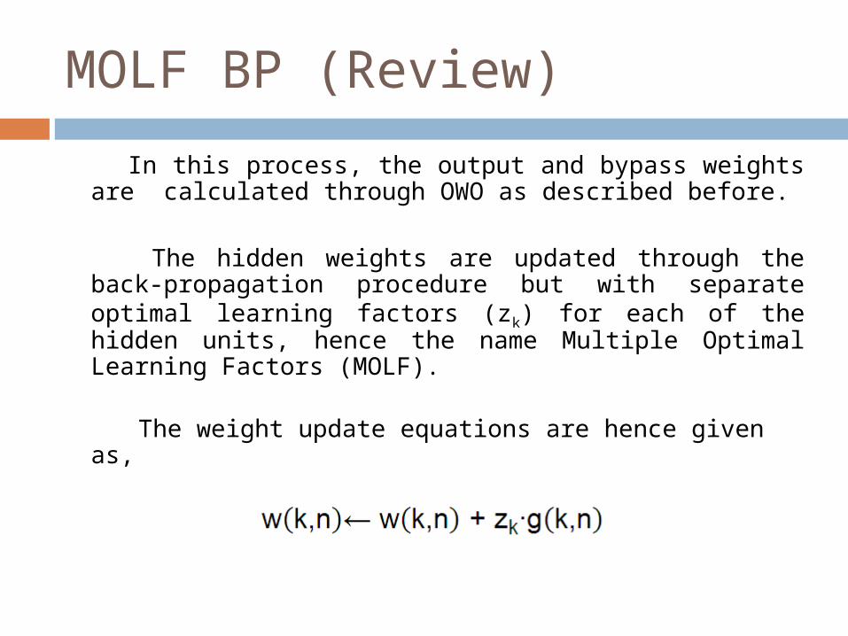
MOLF BP (Review)

In this process, the output and bypass weights are calculated through OWO as described before.

The hidden weights are updated through the back-propagation procedure but with separate optimal learning factors (zk) for each of the hidden units, hence the name Multiple Optimal Learning Factors (MOLF).

The weight update equations are hence given as,

MOLF BP (Review)

The vector z containing each of the optimal learning factors zk is found through Newton’s Method, by solving

where,

Problem : Lack convincing motivation for this approach

Strongly Equivalent networks (New)

Input Layer

Output Layer Hidden Layer

xp (1)

xp (3)

xp (2)

yp (M)

yp (3)

yp (2)

yp (1)

np (Nh) op (Nh)

np (1) op (1)W Woh

Woi

xp (N+1)

Input Layer

Output Layer Hidden Layer

xp (1)

xp (3)

xp (2)

yp (M)

yp (3)

yp (2)

yp (1)

n’p (Nh)op (Nh)

n’p (1) op (1)W’ Woh

Woi

xp (N+1)C

MLP 1 MLP 2

MLP 1 and MLP 2, have identical performance if W = C • W’.

However, they train differently

Goal : To maximize the decrease in error E, with respect to C

Optimal net function transformation (New)

Input Layer

xp (1)

xp (3)xp (2)

xp (N+1) n’p (Nh)

n’p (1)W’

n’p

Cnp (1)np (2)np (3)

np (Nh) np

n’p - Optimal net function vector

np - Actual net function vector

C - Transformation matrix

W = C • W’

xp (1)

xp (3)

xp (2)

xp (N+1)

W np (1)

np (3)

np (Nh)

np (2)

MLP1 weight change equation (New)The MLP 2 weight update equation is W’ = W’ + z•G’ where G’ = CTG, W’

= C-1W

Multiplying by C we get

W = W + z•CCTG , R=CCT

So RG is a valid update for MLP 1Why use MLP 1 ? Because MLP 2 requires C-1

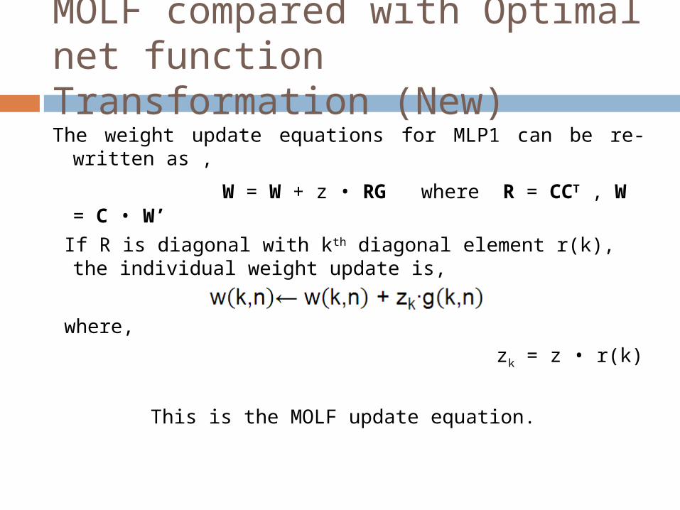
MOLF compared with Optimal net function Transformation (New)

The weight update equations for MLP1 can be re-written as ,

W = W + z • RG where R = CCT , W = C • W’

If R is diagonal with kth diagonal element r(k), the individual weight update is,

where,

zk = z • r(k)

This is the MOLF update equation.

Linearly dependent input layers in MOLF (Review)

Dependent Inputs :

Lemma 1 : Linearly dependent inputs, when added to the network, each element of Hmolf gains some first and second degree terms in the variables b(n).

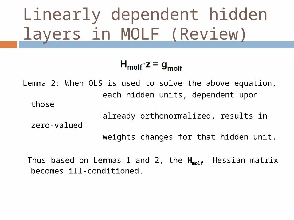
Linearly dependent hidden layers in MOLF (Review)

Lemma 2: When OLS is used to solve the above equation,

each hidden units, dependent upon those

already orthonormalized, results in zero-valued

weights changes for that hidden unit.

Thus based on Lemmas 1 and 2, the Hmolf Hessian matrix becomes ill-conditioned.

Collapsing the MOLF Hessian

Hmolf - MOLF Hessian

Hmolf1 - Collapsed MOLF Hessian

Nh - Number of Hidden units

NOLF - Size of Collapsed MOLF Hessian

Variable Number of OLFs

Collapsing the MOLF Hessian is equivalent to assigning one or more hidden units to each OLF.

New number of OLFs = NOLF

Number of hidden units assigned to an OLF = Nh/NOLF

Advantages :

NOLF can be varied to improve performance or decrease number of multiplies.

The number of multiplies required for computing the OLFs at every iteration, decreases cubically with a decrease in NOLF.

No. of multiplies vs NOLF

0 5 10 15 20 25 30 35 400

1

2

3

4

5

6

7x 10

4

N o

.of M

ultip

lies

NOLF

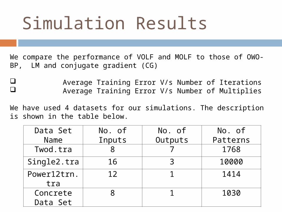
Simulation Results

We compare the performance of VOLF and MOLF to those of OWO-BP, LM and conjugate gradient (CG) Average Training Error V/s Number of Iterations Average Training Error V/s Number of Multiplies

We have used 4 datasets for our simulations. The description is shown in the table below.

Data Set Name No. of Inputs No. of Outputs No. of Patterns

Twod.tra 8 7 1768

Single2.tra 16 3 10000

Power12trn.tra 12 1 1414

Concrete Data Set

8 1 1030

Simulation conditions

Different numbers of hidden units are chosen for each data file based on network pruning to minimize validation error.

The K-fold validation procedure is used to calculate the average training and validation errors.

Given a data set, it is split into K non-overlapping parts of equal size, and (K − 1) parts are used for training and the remaining one part for validation. The procedure is repeated till all k combinations have been exhausted. (K = 10 for our simulations) e In all our simulations we have 4000 iterations for the first order algorithms BP-OLF and CG, 4000 iterations for MOLF and VOLF and for LM we have 300 iterations. In each experiment, each algorithm uses the same initial network.

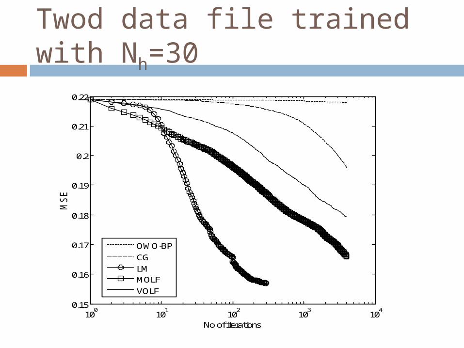
Twod data file trained with Nh=30

100

101

102

103

104

0.15

0.16

0.17

0.18

0.19

0.2

0.21

0.22

MS

E

No of iterations

OWO-BP

CG

LMMOLF

VOLF

Twod data file trained with Nh=30

106

107

108

109

1010

1011

1012

0.15

0.16

0.17

0.18

0.19

0.2

0.21

0.22

No of Multiplies

MS

E

OWO-BP

CG

LMMOLF

VOLF

Single2 data file with Nh=20

100

101

102

103

104

0

0.1

0.2

0.3

0.4

0.5

0.6

0.7

0.8

0.9

No of Iterations

MS

E

OWO-BP

CG

LMMOLF

VOLF

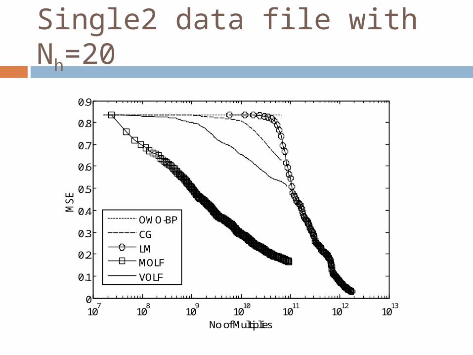
Single2 data file with Nh=20

107

108

109

1010

1011

1012

1013

0

0.1

0.2

0.3

0.4

0.5

0.6

0.7

0.8

0.9

No of Multiplies

MS

E

OWO-BP

CG

LMMOLF

VOLF

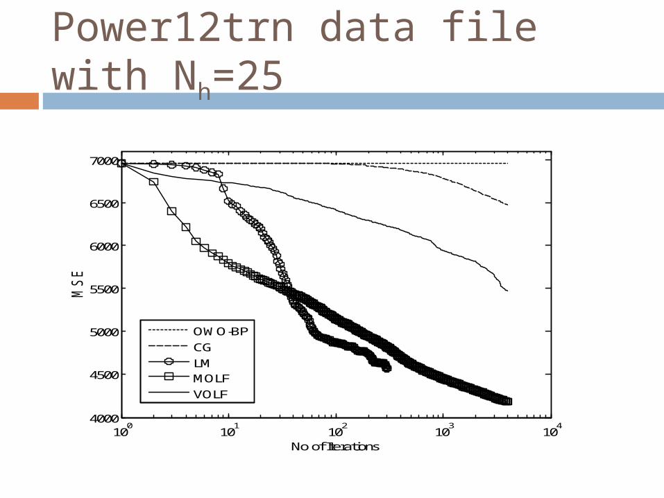
Power12trn data file with Nh=25

100

101

102

103

104

4000

4500

5000

5500

6000

6500

7000

No of Iterations

MS

E

OWO-BP

CG

LMMOLF

VOLF

Power12trn data file with Nh=25

106

107

108

109

1010

1011

1012

4000

4500

5000

5500

6000

6500

7000

No of Multiplies

MS

E

OWO-BP

CG

LMMOLF

VOLF

Concrete data file with Nh=15

100

101

102

103

104

10

20

30

40

50

60

70

No of Iterations

MS

E

OWO-BP

CG

LMMOLF

VOLF

Concrete data file with Nh=15

105

106

107

108

109

1010

1011

10

20

30

40

50

60

70

No of Multiplies

MS

E

OWO-BP

CG

LMMOLF

VOLF

Conclusions

The error found from the VOLF algorithm lies between the errors produced by the MOLF and OWO-BP algorithms based on the value of NOLF chosen

The VOLF and MOLF algorithms are found to produce good results approaching that of the LM algorithm, with computational requirements only in the order of first order training algorithms.

Future Work

Applying MOLF to more than one hidden layer.

Converting the proposed algorithm into a

single–stage procedure where all the weights

are updated simultaneously.

References

R. C. Odom, P. Pavlakos, S.S. Diocee, S. M. Bailey, D. M. Zander, and J. J. Gillespie, “Shaly sand analysis using density-neutron porosities from a cased-hole pulsed neutron system,” SPE Rocky Mountain regional meeting proceedings: Society of Petroleum Engineers, pp. 467-476, 1999.

A. Khotanzad, M. H. Davis, A. Abaye, D. J. Maratukulam, “An artificial neural network hourly temperature forecaster with applications in load forecasting,” IEEE Transactions on Power Systems, vol. 11, No. 2, pp. 870-876, May 1996.

S. Marinai, M. Gori, G. Soda, “Artificial neural networks for document analysis and recognition,” IEEE Transactions on Pattern Analysis and Machine Intelligence, vol. 27, No. 1, pp. 23-35, 2005.

J. Kamruzzaman, R. A. Sarker, R. Begg, Artificial Neural Networks: Applications in Finance and Manufacturing, Idea Group Inc (IGI), 2006.

L. Wang and X. Fu, Data Mining With Computational Intelligence, Springer-Verlag, 2005. K. Hornik, M. Stinchcombe, and H.White, “Multilayer Feedforward Networks Are Universal

Approximators.” Neural Networks, Vol. 2, No. 5, 1989, pp.359-366. K. Hornik, M. Stinchcombe, and H. White, “Universal Approximation of an Unknown Mapping

and its Derivatives Using Multilayer Feedforward Networks,” Neural Networks,vol. 3,1990, pp.551-560.

Michael T.Manry, Steven J.Apollo, and Qiang Yu, “Minimum Mean Square Estimation and Neural Networks,” Neurocomputing, vol. 13, September 1996, pp.59-74.

G. Cybenko, “Approximations by superposition of a sigmoidal function,” Mathematics of Control, Signals, and Systems (MCSS), vol. 2, pp. 303-314, 1989.

References continued

D. W. Ruck et al., “The multi-layer perceptron as an approximation to a Bayes optimal discriminant function,” IEEE Transactions on Neural Networks, vol. 1, No. 4, 1990.

Q. Yu, S.J. Apollo, and M.T. Manry, “MAP estimation and the multi-layer perceptron,” Proceedings of the 1993 IEEE Workshop on Neural Networks for Signal Processing, pp. 30-39, Linthicum Heights, Maryland, Sept. 6-9, 1993.

D.E. Rumelhart, G.E. Hinton, and R.J. Williams, “Learning internal representations by error propagation,” in D.E. Rumelhart and J.L. McClelland (Eds.), Parallel Distributed Processing, vol. I, Cambridge, Massachusetts: The MIT Press, 1986.

J.P. Fitch, S.K. Lehman, F.U. Dowla, S.Y. Lu, E.M. Johansson, and D.M. Goodman, "Ship Wake-Detection Procedure Using Conjugate Gradient Trained Artificial Neural Networks," IEEE Trans. on Geoscience and Remote Sensing, Vol. 29, No. 5, September 1991, pp. 718-726.

Changhua Yu, Michael T. Manry, and Jiang Li, "Effects of nonsingular pre-processing on feed-forward network training ". International Journal of Pattern Recognition and Artificial Intelligence , Vol. 19, No. 2 (2005) pp. 217-247.

S. McLoone and G. Irwin, “A variable memory Quasi-Newton training algorithm,” Neural Processing Letters, vol. 9, pp. 77-89, 1999.

A. J. Shepherd Second-Order Methods for Neural Networks, Springer-Verlag New York, Inc., 1997.

K. Levenberg, “A method for the solution of certain problems in least squares,” Quart. Appl. Math., Vol. 2, pp. 164.168, 1944.

References continued

G. D. Magoulas, M. N. Vrahatis, and G. S. Androulakis, ”Improving the Convergence of the Backpropagation Algorithm Using Learning Rate Adaptation Methods,” Neural Computation, Vol. 11, No. 7, Pages 1769-1796, October 1, 1999.

Sanjeev Malalur, M. T. Manry, "Multiple Optimal Learning Factors for Feed-forward Networks," accepted by The SPIE Defense, Security and Sensing (DSS) Conference, Orlando, FL, April 2010

W. Kaminski, P. Strumillo, “Kernel orthonormalization in radial basis function neural networks,” IEEE Transactions on Neural Networks, vol. 8, Issue 5, pp. 1177 - 1183, 1997

D.E Rumelhart, G.E. Hinton, and R.J. Williams, “Learning representations of back-propagation errors,” Nature, London, 1986, vol. 323, pp. 533-536

D.B.Parker, “Learning Logic,” Invention Report S81-64,File 1, Office of Technology Licensing, Stanford Univ., 1982

T.H. Kim “Development and Evaluation of Multilayer Perceptron Training Algorithms”, Phd. Dissertation, The University of Texas at Arlington, 2001.

S.A. Barton, “A matrix method for optimizing a neural network,” Neural Computation, vol. 3, no. 3, pp. 450-459, 1991.

Nocedal, Jorge & Wright, Stephen J. (1999). Numerical Optimization. Springer-Verlag Bonnans, J. F., Gilbert, J.Ch., Lemaréchal, C and Sagastizábal, C.A. (2006), Numerical

optimization, theoretical and numerical aspects.Second edition. Springer.

References continued

R. Fletcher, "Conjugate Direction Methods," chapter 5 in Numerical Methods for Unconstrained Optimization, edited by W. Murray, Academic Press, New York, 1972.

P.E. Gill, W. Murray, and M.H. Wright, Practical Optimization, Academic Press, New York,1981.

Charytoniuk, W.; Chen, M.-S.; "Very short-term load forecasting using artificial neural networks ," Power Systems, IEEE Transactions on , vol.15, no.1, pp.263-268, Feb 2000

Ning Wang; Xianyao Meng; Yiming Bai;,"A fast and compact fuzzy neural network for online extraction of fuzzy rules," Control and Decision Conference, 2009. CCDC '09. Chinese , vol.,no.,pp.4249-4254,17-19 June 2009

Wei Wu; Guorui Feng; Zhengxue Li; Yuesheng Xu; , "Deterministic convergence of an online gradient method for BP neural networks," Neural Networks, IEEE Transactions on , vol.16, no.3, pp.533-540, May 2005

Saurabh Sureka, Michael Manry, A Functional Link Network With Ordered Basis Functions, Proceedings of International Joint Conference on Neural Networks, Orlando, Florida, USA, August 12-17, 2007.

Lee, Y.; Oh, S.-H,; Kim, M.W., “The effect of initial weights on premature saturation in back-propagation learning,” Neural Networks, 1991., IJCNN-91-Seattle International Joint Conference on, vol.1, 1991 pp. 765-770 vol. 1

P.L Narasimha, S. Malalur, and M.T. Manry, Small Models of Large Machines, Proceedings of the TwentyFirst International Conference of the Florida Al Research Society, pp.83-88, May 2008.

References continued

Pramod L. Narasimha, Walter H. Delashmit, Michael T. Manry, Jiang Li, Francisco Maldonado, An integrated growing-pruning method for feedforward network training, Neurocomputing vol. 71, pp. 2831–2847, 2008.

R.P Lippman, “An introduction to computing with Neural Nets,” IEEE ASSP Magazine,April 1987.

S. S. Malalur and M. T. Manry, Feedforward Network Training Using Optimal Input Gains, Proc.of IJCNN’09, Atlanta, Georgia, pp. 1953-1960, June 14-19, 2009.

Univ. of Texas at Arlington, Training Data Files – http://wwwee.uta.edu/eeweb/ip/training_ data_files.html.

Univ. of California, Irvine, Machine Learning Repository - http://archive.ics.uci.edu/ml/

Questions