
Actuariat IARD - ACT2040 Partie 7 - provisions pour ...freakonometrics.free.fr/slides-2040-7.pdf ·...
90
11pt Arthur CHARPENTIER - ACT2040 - Actuariat IARD - Hiver 2013 Actuariat IARD - ACT2040 Partie 7 - provisions pour sinistres à payer, IBNR et triangles Arthur Charpentier [email protected] http ://freakonometrics.hypotheses.org/ Hiver 2013 1
Transcript of Actuariat IARD - ACT2040 Partie 7 - provisions pour ...freakonometrics.free.fr/slides-2040-7.pdf ·...
11pt
11pt
Note Exemple Exemple
11pt
Preuve
Arthur CHARPENTIER - ACT2040 - Actuariat IARD - Hiver 2013
Actuariat IARD - ACT2040Partie 7 - provisions pour sinistres
à payer, IBNR et triangles
Arthur Charpentier
http ://freakonometrics.hypotheses.org/
Hiver 2013
1
Arthur CHARPENTIER - ACT2040 - Actuariat IARD - Hiver 2013
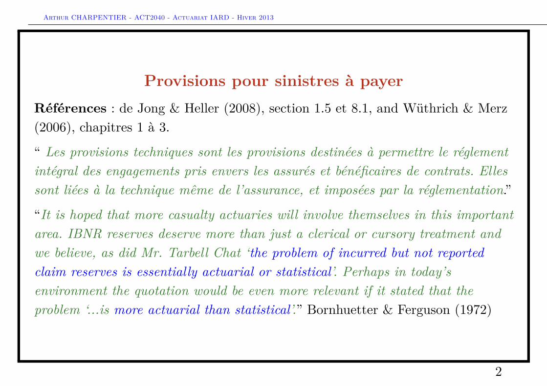
Provisions pour sinistres à payerRéférences : de Jong & Heller (2008), section 1.5 et 8.1, and Wüthrich & Merz(2006), chapitres 1 à 3.
“ Les provisions techniques sont les provisions destinées à permettre le réglementintégral des engagements pris envers les assurés et bénéficaires de contrats. Ellessont liées à la technique même de l’assurance, et imposées par la réglementation.”
“It is hoped that more casualty actuaries will involve themselves in this importantarea. IBNR reserves deserve more than just a clerical or cursory treatment andwe believe, as did Mr. Tarbell Chat ‘the problem of incurred but not reportedclaim reserves is essentially actuarial or statistical’. Perhaps in today’senvironment the quotation would be even more relevant if it stated that theproblem ‘...is more actuarial than statistical’.” Bornhuetter & Ferguson (1972)
2
Arthur CHARPENTIER - ACT2040 - Actuariat IARD - Hiver 2013
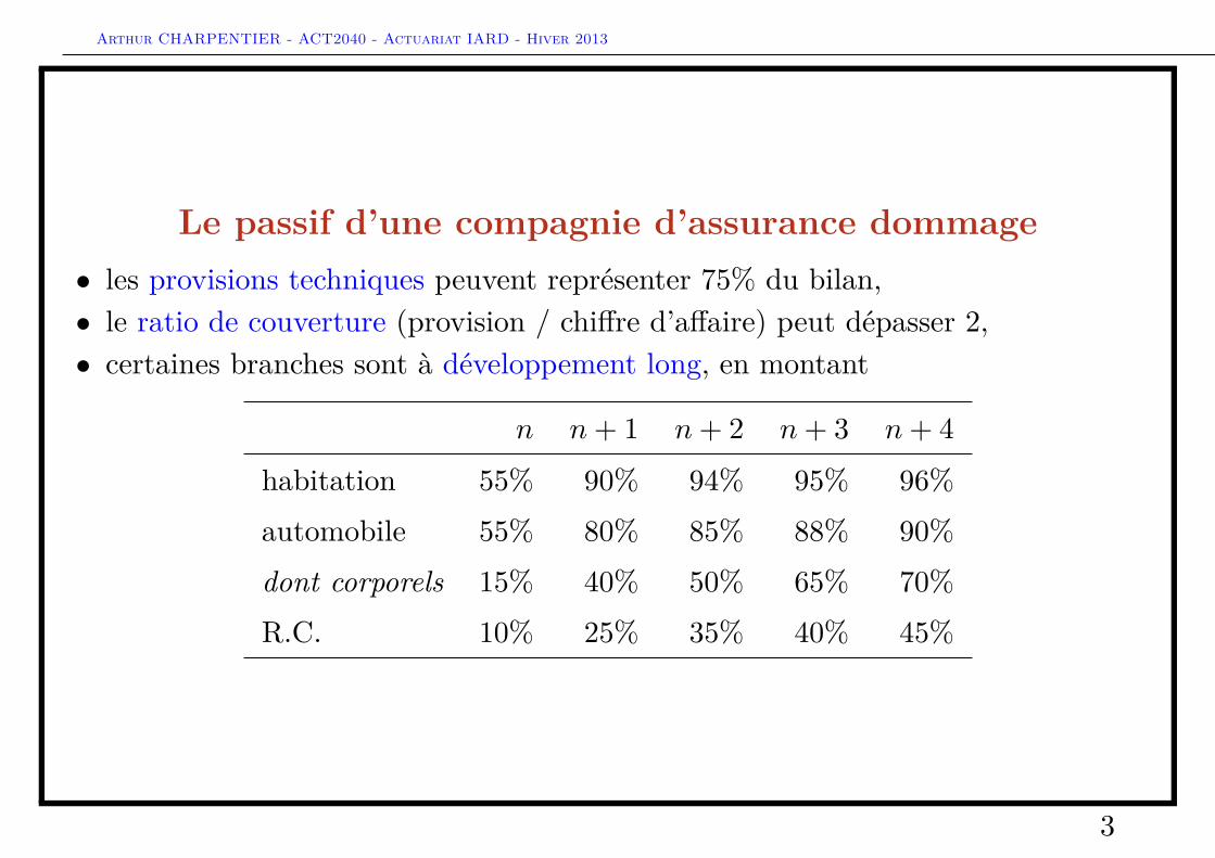
Le passif d’une compagnie d’assurance dommage• les provisions techniques peuvent représenter 75% du bilan,• le ratio de couverture (provision / chiffre d’affaire) peut dépasser 2,• certaines branches sont à développement long, en montant
n n+ 1 n+ 2 n+ 3 n+ 4
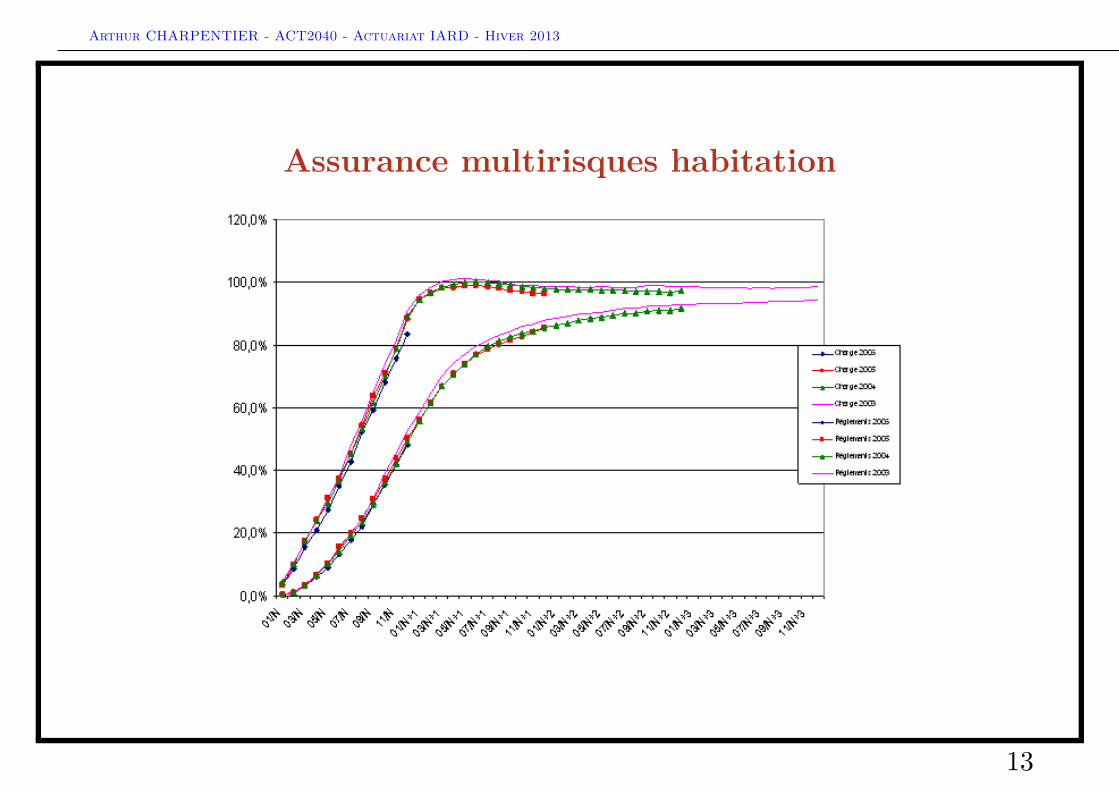
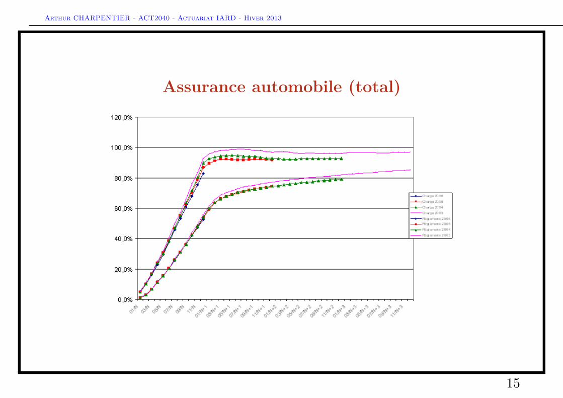
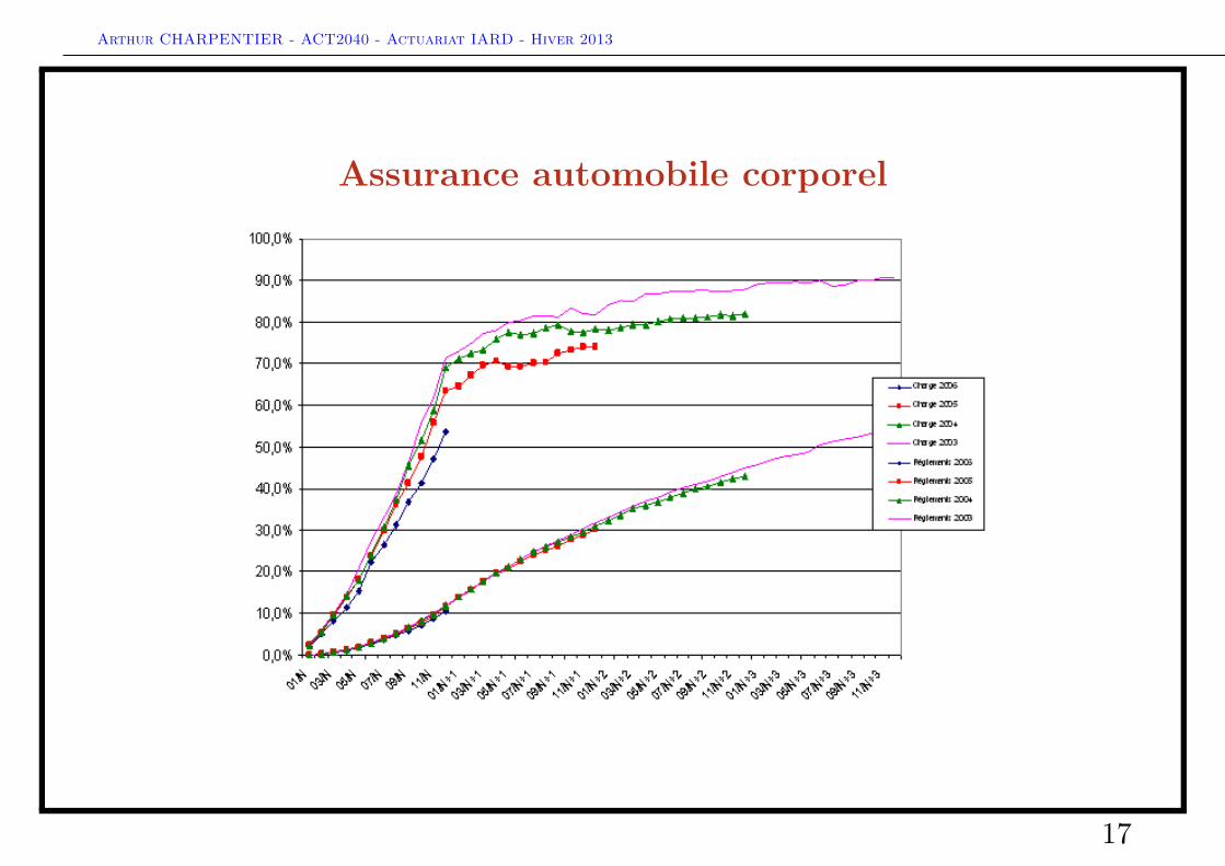
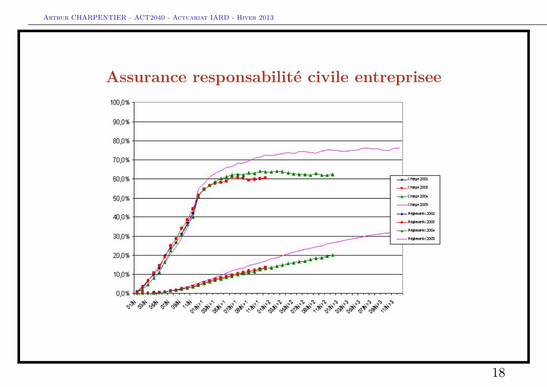
habitation 55% 90% 94% 95% 96%automobile 55% 80% 85% 88% 90%dont corporels 15% 40% 50% 65% 70%R.C. 10% 25% 35% 40% 45%
3

Arthur CHARPENTIER - ACT2040 - Actuariat IARD - Hiver 2013
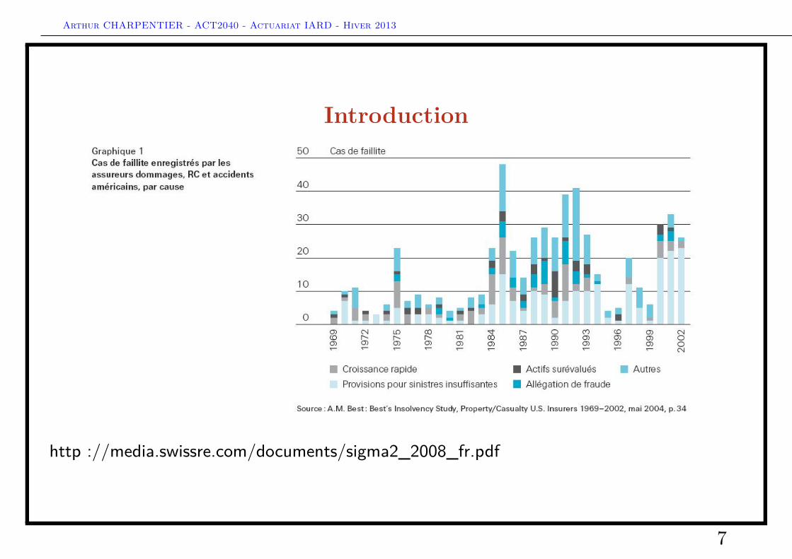
Introduction
http ://media.swissre.com/documents/sigma2_2008_fr.pdf
4

Arthur CHARPENTIER - ACT2040 - Actuariat IARD - Hiver 2013
Introduction
http ://media.swissre.com/documents/sigma2_2008_fr.pdf
5

Arthur CHARPENTIER - ACT2040 - Actuariat IARD - Hiver 2013
Introduction
http ://media.swissre.com/documents/sigma2_2008_fr.pdf
6
Arthur CHARPENTIER - ACT2040 - Actuariat IARD - Hiver 2013
Introduction
http ://media.swissre.com/documents/sigma2_2008_fr.pdf
7
Arthur CHARPENTIER - ACT2040 - Actuariat IARD - Hiver 2013
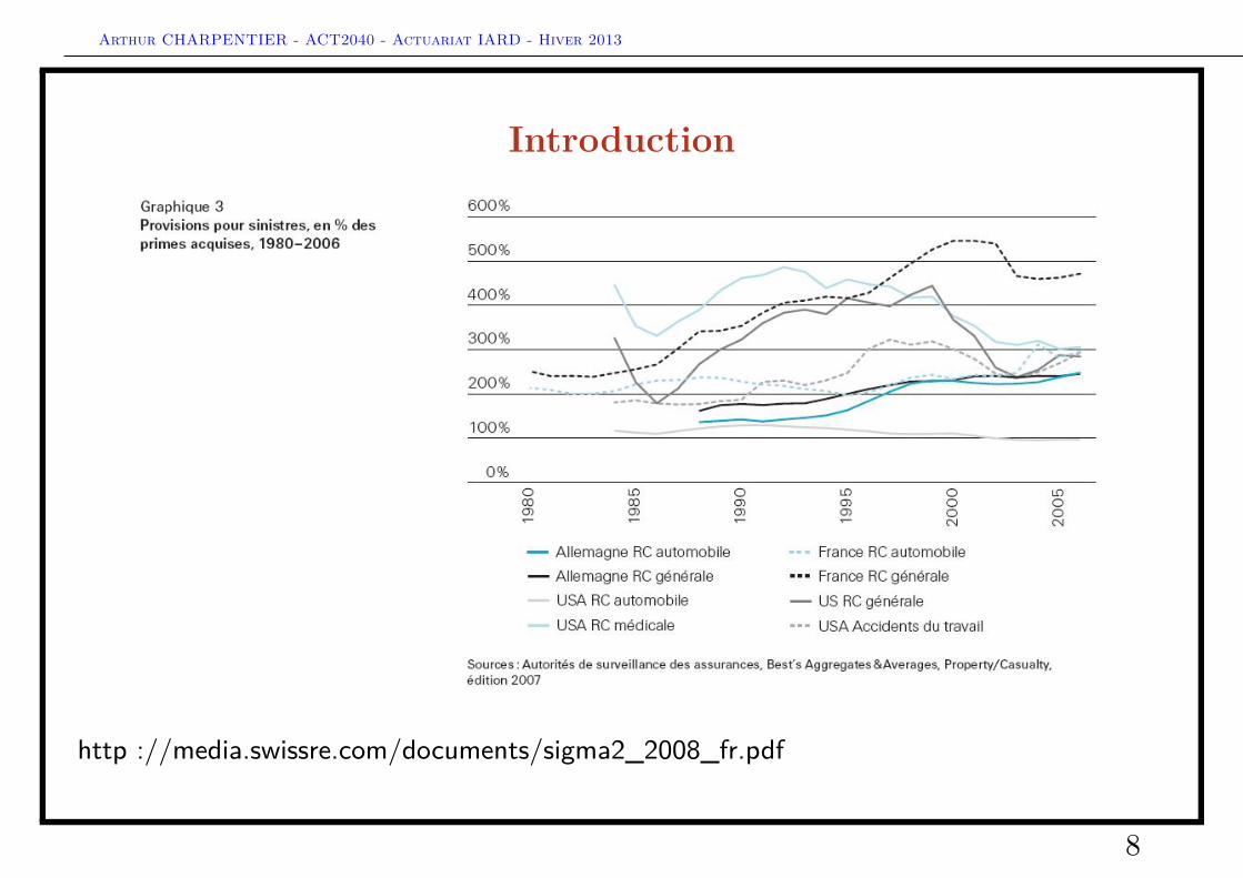
Introduction
http ://media.swissre.com/documents/sigma2_2008_fr.pdf
8
Arthur CHARPENTIER - ACT2040 - Actuariat IARD - Hiver 2013
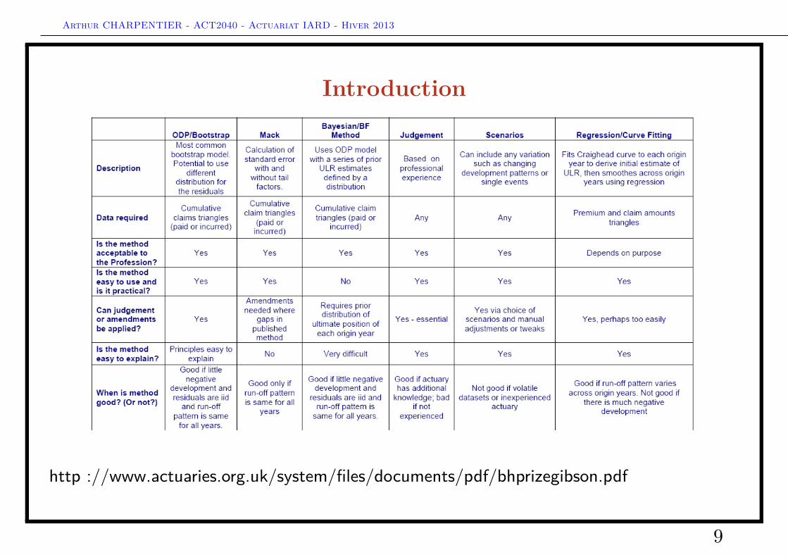
Introduction
http ://www.actuaries.org.uk/system/files/documents/pdf/bhprizegibson.pdf
9

Arthur CHARPENTIER - ACT2040 - Actuariat IARD - Hiver 2013
Introduction
http ://www.actuaries.org.uk/system/files/documents/pdf/bhprizegibson.pdf
10
Arthur CHARPENTIER - ACT2040 - Actuariat IARD - Hiver 2013
Introduction
http ://www.actuaries.org.uk/system/files/documents/pdf/bhprizegibson.pdf
11
Arthur CHARPENTIER - ACT2040 - Actuariat IARD - Hiver 2013
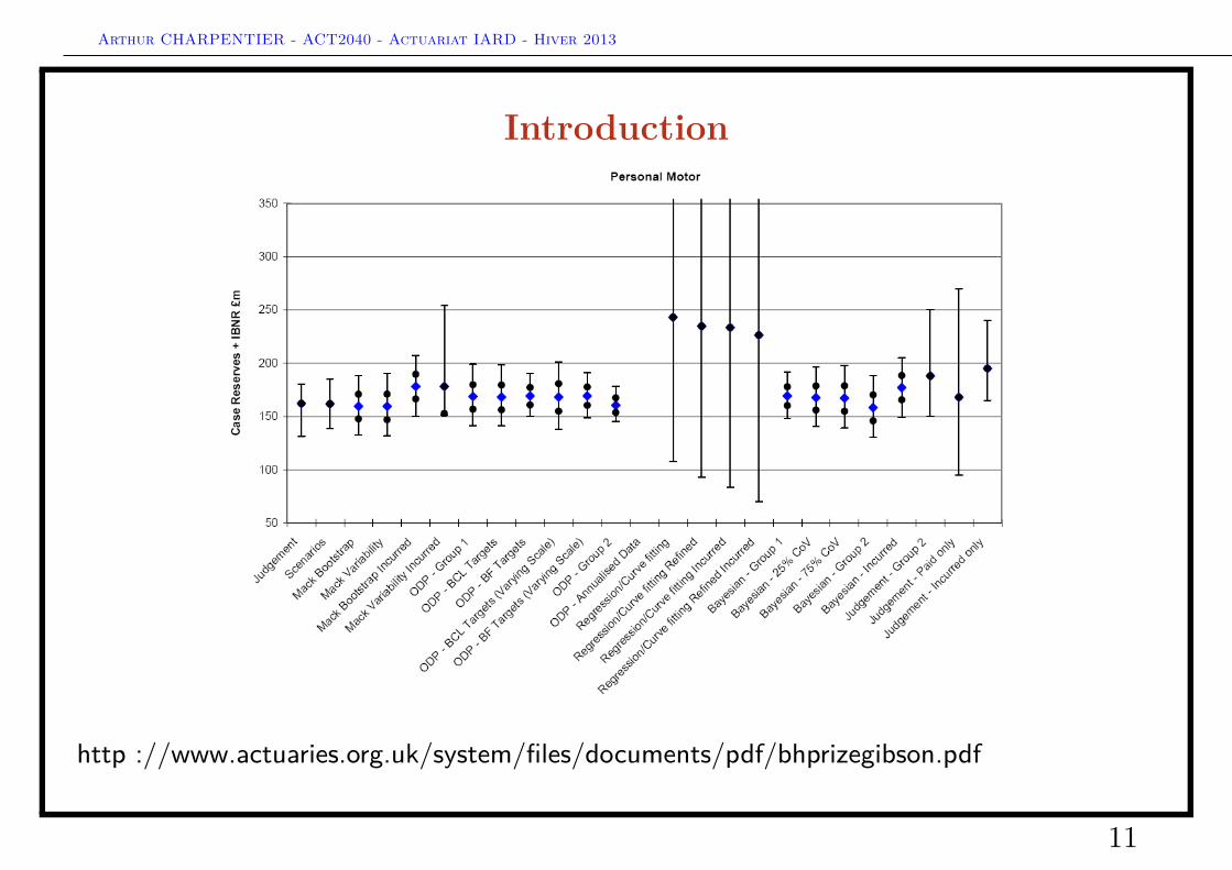
Introduction
http ://www.actuaries.org.uk/system/files/documents/pdf/bhprizegibson.pdf
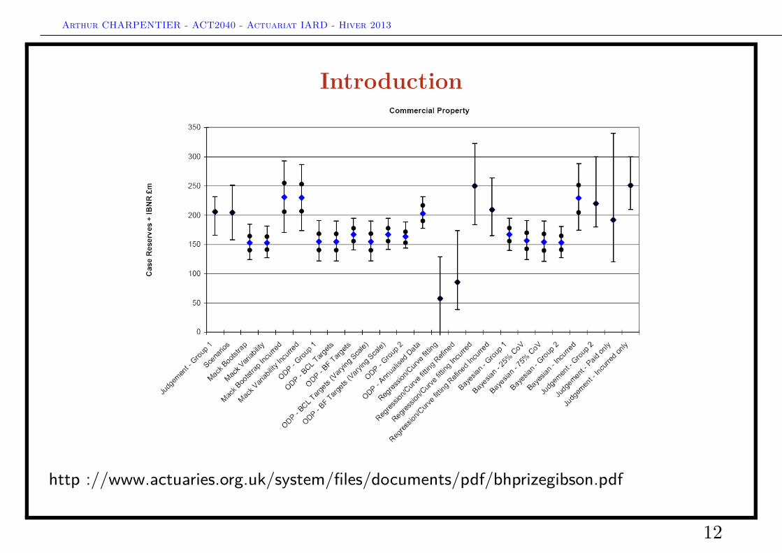
12
Arthur CHARPENTIER - ACT2040 - Actuariat IARD - Hiver 2013
Assurance multirisques habitation
13

Arthur CHARPENTIER - ACT2040 - Actuariat IARD - Hiver 2013
Assurance risque incendies entreprises
14
Arthur CHARPENTIER - ACT2040 - Actuariat IARD - Hiver 2013
Assurance automobile (total)
15

Arthur CHARPENTIER - ACT2040 - Actuariat IARD - Hiver 2013
Assurance automobile matériel
16
Arthur CHARPENTIER - ACT2040 - Actuariat IARD - Hiver 2013
Assurance automobile corporel
17
Arthur CHARPENTIER - ACT2040 - Actuariat IARD - Hiver 2013
Assurance responsabilité civile entreprisee
18
Arthur CHARPENTIER - ACT2040 - Actuariat IARD - Hiver 2013
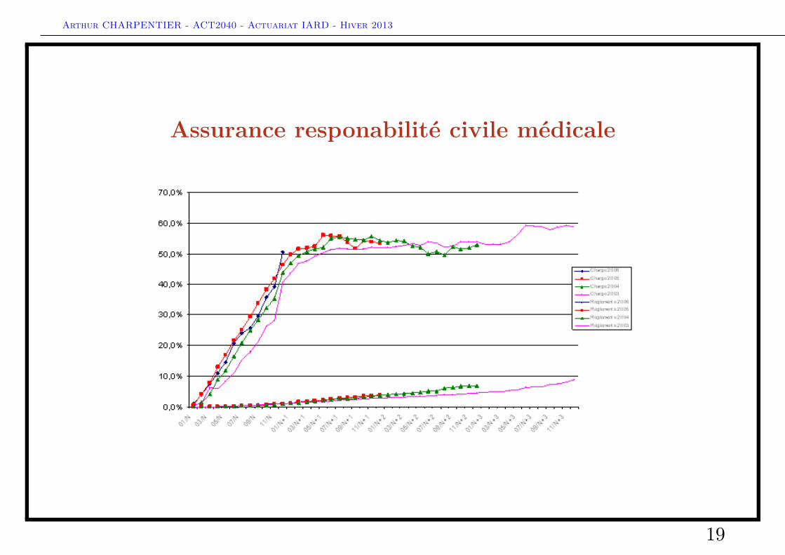
Assurance responabilité civile médicale
19
Arthur CHARPENTIER - ACT2040 - Actuariat IARD - Hiver 2013
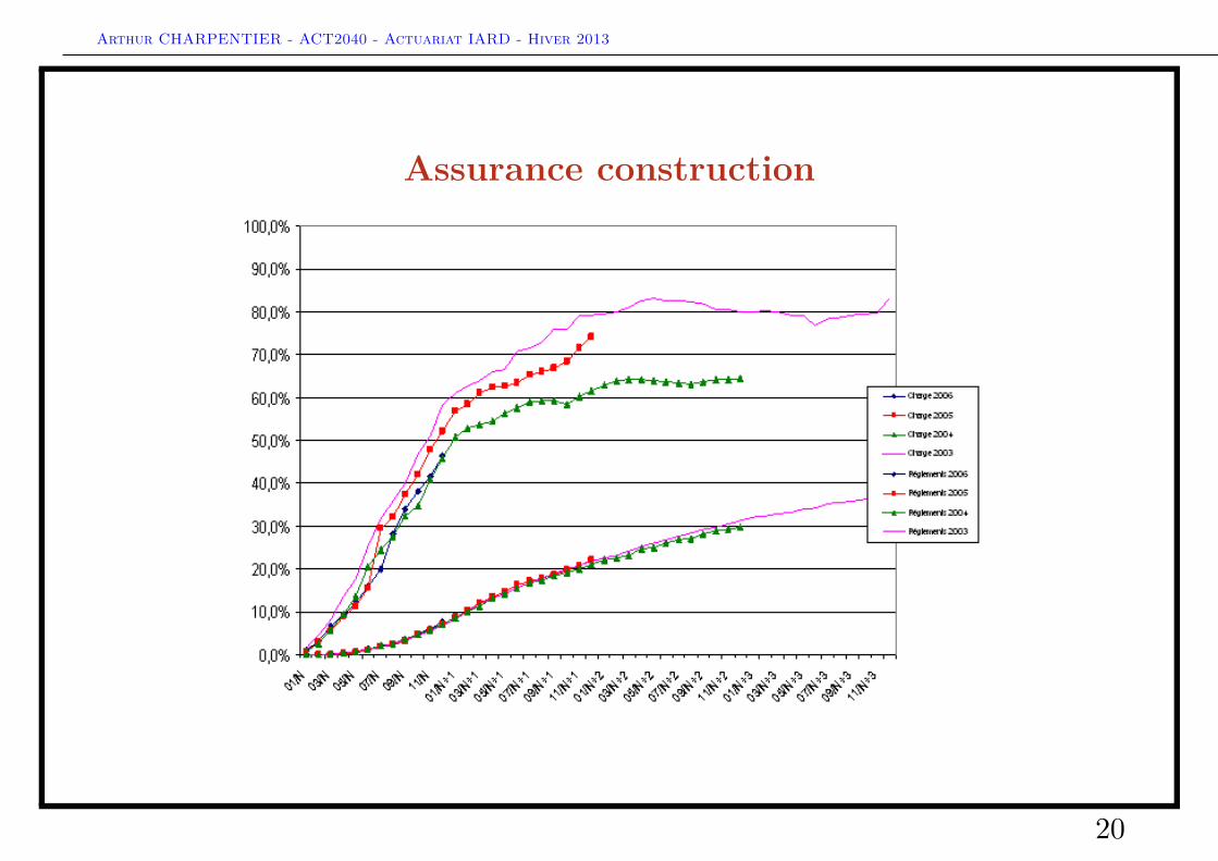
Assurance construction
20
Arthur CHARPENTIER - ACT2040 - Actuariat IARD - Hiver 2013
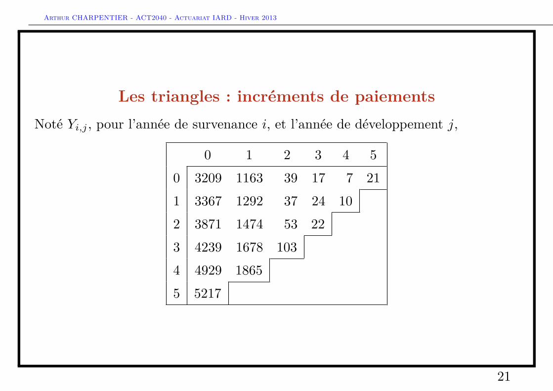
Les triangles : incréments de paiementsNoté Yi,j , pour l’année de survenance i, et l’année de développement j,
0 1 2 3 4 50 3209 1163 39 17 7 211 3367 1292 37 24 102 3871 1474 53 223 4239 1678 1034 4929 18655 5217
21
Arthur CHARPENTIER - ACT2040 - Actuariat IARD - Hiver 2013
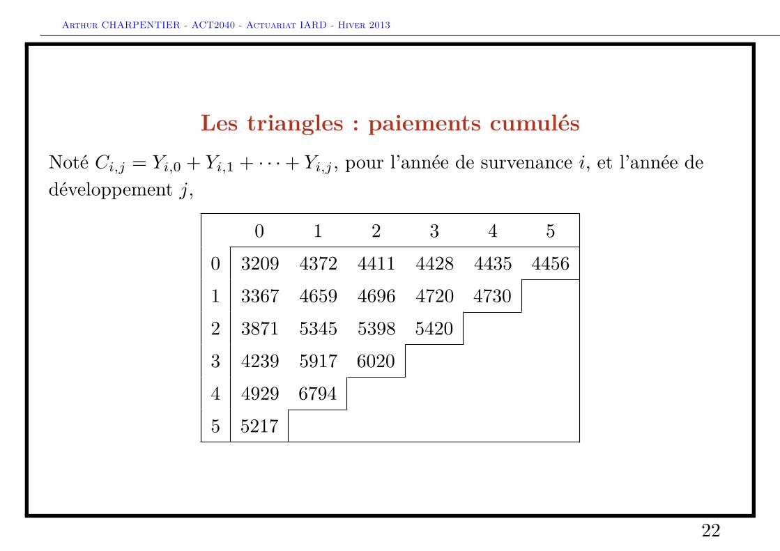
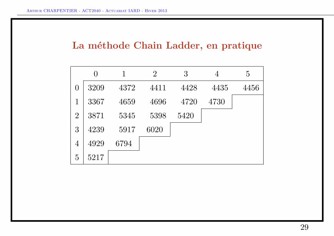
Les triangles : paiements cumulésNoté Ci,j = Yi,0 + Yi,1 + · · ·+ Yi,j , pour l’année de survenance i, et l’année dedéveloppement j,
0 1 2 3 4 50 3209 4372 4411 4428 4435 44561 3367 4659 4696 4720 47302 3871 5345 5398 54203 4239 5917 60204 4929 67945 5217
22
Arthur CHARPENTIER - ACT2040 - Actuariat IARD - Hiver 2013
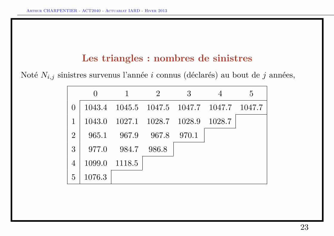
Les triangles : nombres de sinistresNoté Ni,j sinistres survenus l’année i connus (déclarés) au bout de j années,
0 1 2 3 4 50 1043.4 1045.5 1047.5 1047.7 1047.7 1047.71 1043.0 1027.1 1028.7 1028.9 1028.72 965.1 967.9 967.8 970.13 977.0 984.7 986.84 1099.0 1118.55 1076.3
23
Arthur CHARPENTIER - ACT2040 - Actuariat IARD - Hiver 2013
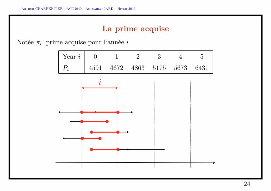
La prime acquiseNotée πi, prime acquise pour l’année i
Year i 0 1 2 3 4 5Pi 4591 4672 4863 5175 5673 6431
24
Arthur CHARPENTIER - ACT2040 - Actuariat IARD - Hiver 2013
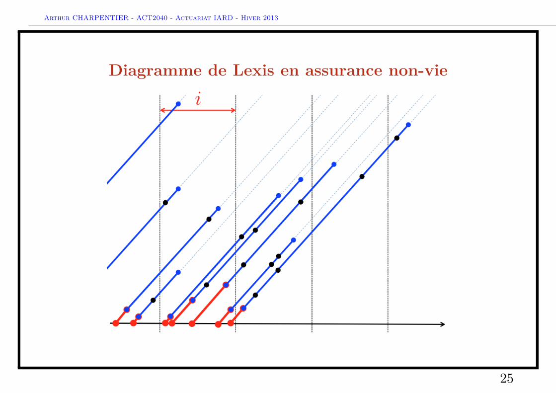
Diagramme de Lexis en assurance non-vie
25
Arthur CHARPENTIER - ACT2040 - Actuariat IARD - Hiver 2013
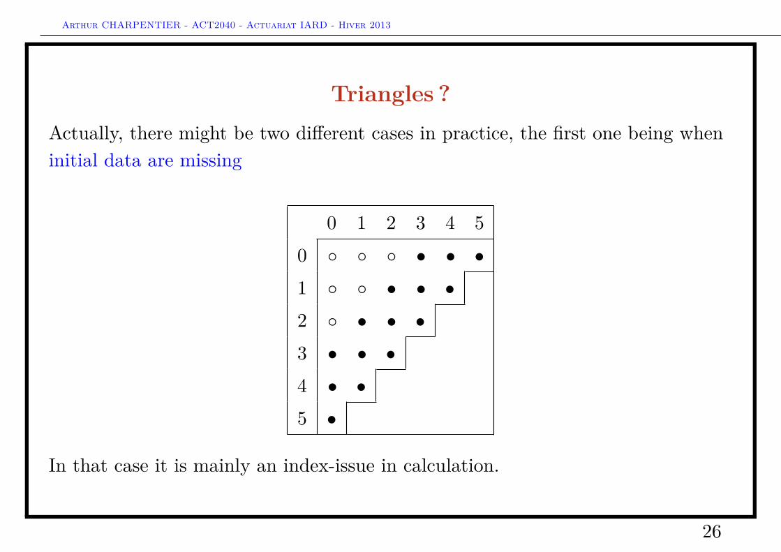
Triangles ?Actually, there might be two different cases in practice, the first one being wheninitial data are missing
0 1 2 3 4 50 ◦ ◦ ◦ • • •1 ◦ ◦ • • •2 ◦ • • •3 • • •4 • •5 •
In that case it is mainly an index-issue in calculation.
26
Arthur CHARPENTIER - ACT2040 - Actuariat IARD - Hiver 2013
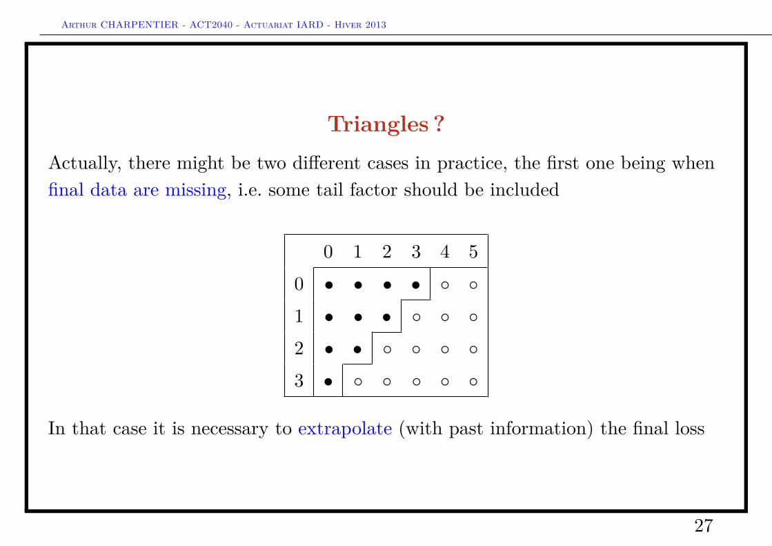
Triangles ?Actually, there might be two different cases in practice, the first one being whenfinal data are missing, i.e. some tail factor should be included
0 1 2 3 4 50 • • • • ◦ ◦1 • • • ◦ ◦ ◦2 • • ◦ ◦ ◦ ◦3 • ◦ ◦ ◦ ◦ ◦
In that case it is necessary to extrapolate (with past information) the final loss
27
Arthur CHARPENTIER - ACT2040 - Actuariat IARD - Hiver 2013
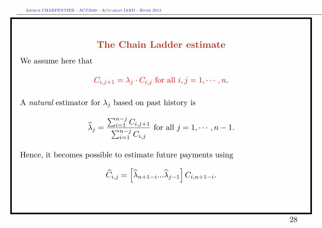
The Chain Ladder estimateWe assume here that
Ci,j+1 = λj · Ci,j for all i, j = 1, · · · , n.
A natural estimator for λj based on past history is
λj =∑n−ji=1 Ci,j+1∑n−ji=1 Ci,j
for all j = 1, · · · , n− 1.
Hence, it becomes possible to estimate future payments using
Ci,j =[λn+1−i...λj−1
]Ci,n+1−i.
28
Arthur CHARPENTIER - ACT2040 - Actuariat IARD - Hiver 2013
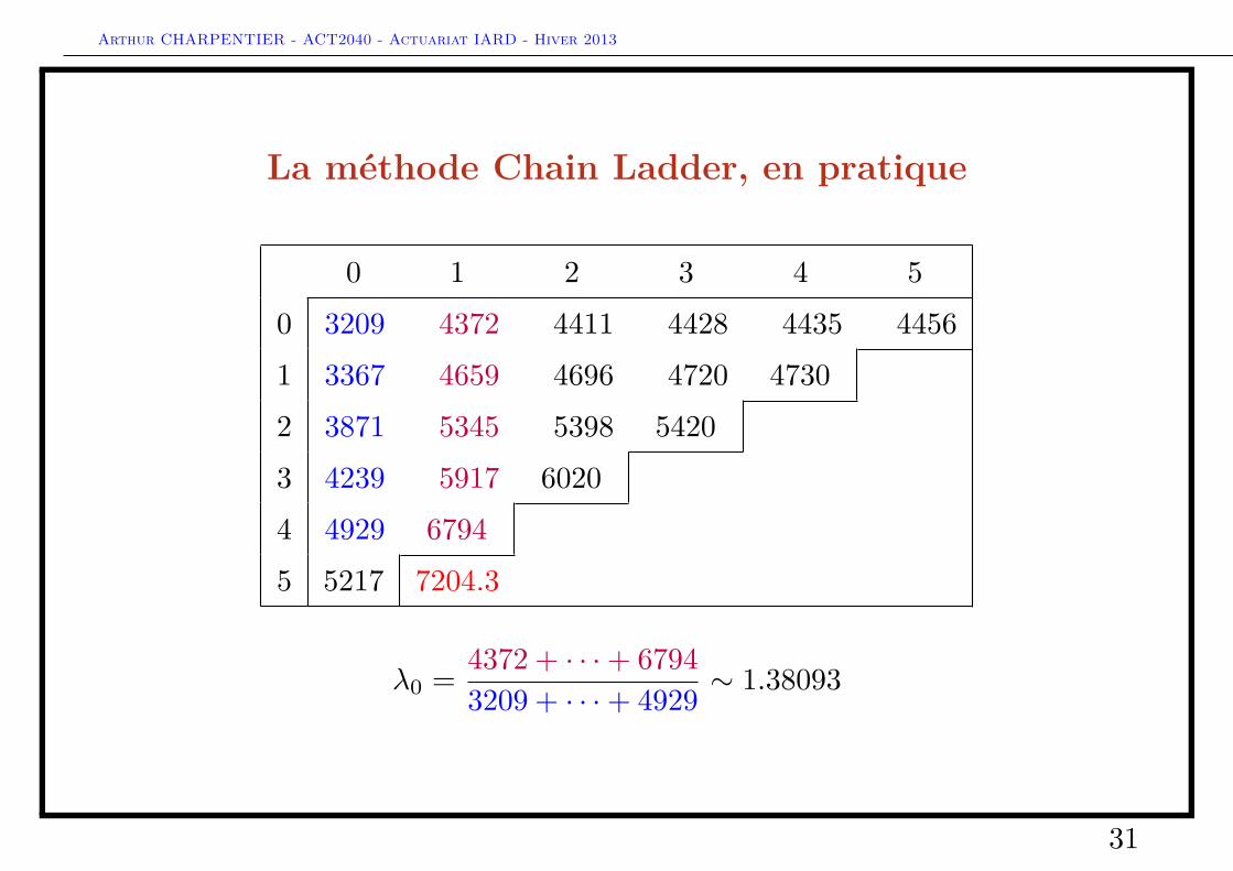
La méthode Chain Ladder, en pratique
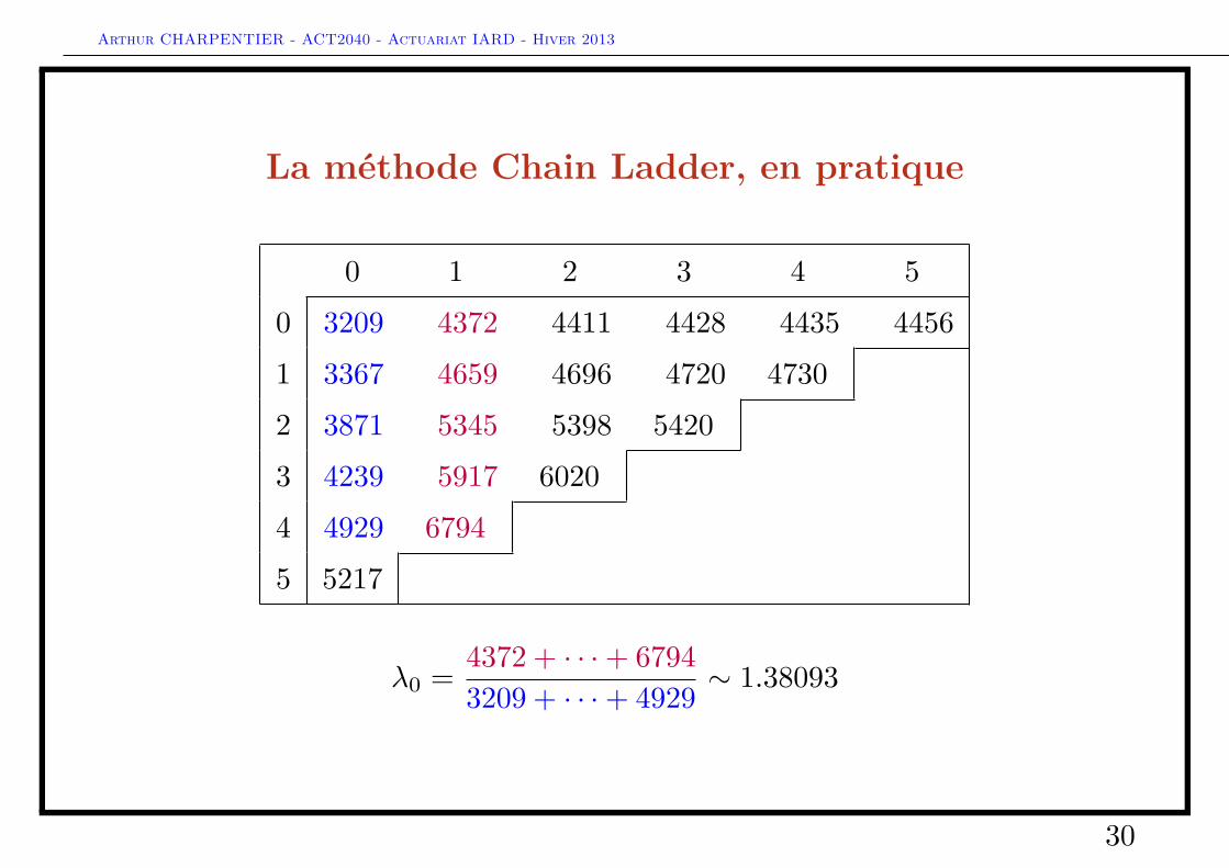
0 1 2 3 4 50 3209 4372 4411 4428 4435 44561 3367 4659 4696 4720 4730 4752.42 3871 5345 5398 5420 5430.1 5455.83 4239 5917 6020 6046.1 6057.4 6086.14 4929 6794 6871.7 6901.5 6914.3 6947.15 5217 7204.3 7286.7 7318.3 7331.9 7366.7
λ0 = 4372 + · · ·+ 67943209 + · · ·+ 4929 ∼ 1.38093
29
Arthur CHARPENTIER - ACT2040 - Actuariat IARD - Hiver 2013
La méthode Chain Ladder, en pratique
0 1 2 3 4 50 3209 4372 4411 4428 4435 44561 3367 4659 4696 4720 4730 4752.42 3871 5345 5398 5420 5430.1 5455.83 4239 5917 6020 6046.1 6057.4 6086.14 4929 6794 6871.7 6901.5 6914.3 6947.15 5217 7204.3 7286.7 7318.3 7331.9 7366.7
λ0 = 4372 + · · ·+ 67943209 + · · ·+ 4929 ∼ 1.38093
30
Arthur CHARPENTIER - ACT2040 - Actuariat IARD - Hiver 2013
La méthode Chain Ladder, en pratique
0 1 2 3 4 50 3209 4372 4411 4428 4435 44561 3367 4659 4696 4720 4730 4752.42 3871 5345 5398 5420 5430.1 5455.83 4239 5917 6020 6046.1 6057.4 6086.14 4929 6794 6871.7 6901.5 6914.3 6947.15 5217 7204.3 7286.7 7318.3 7331.9 7366.7
λ0 = 4372 + · · ·+ 67943209 + · · ·+ 4929 ∼ 1.38093
31
Arthur CHARPENTIER - ACT2040 - Actuariat IARD - Hiver 2013
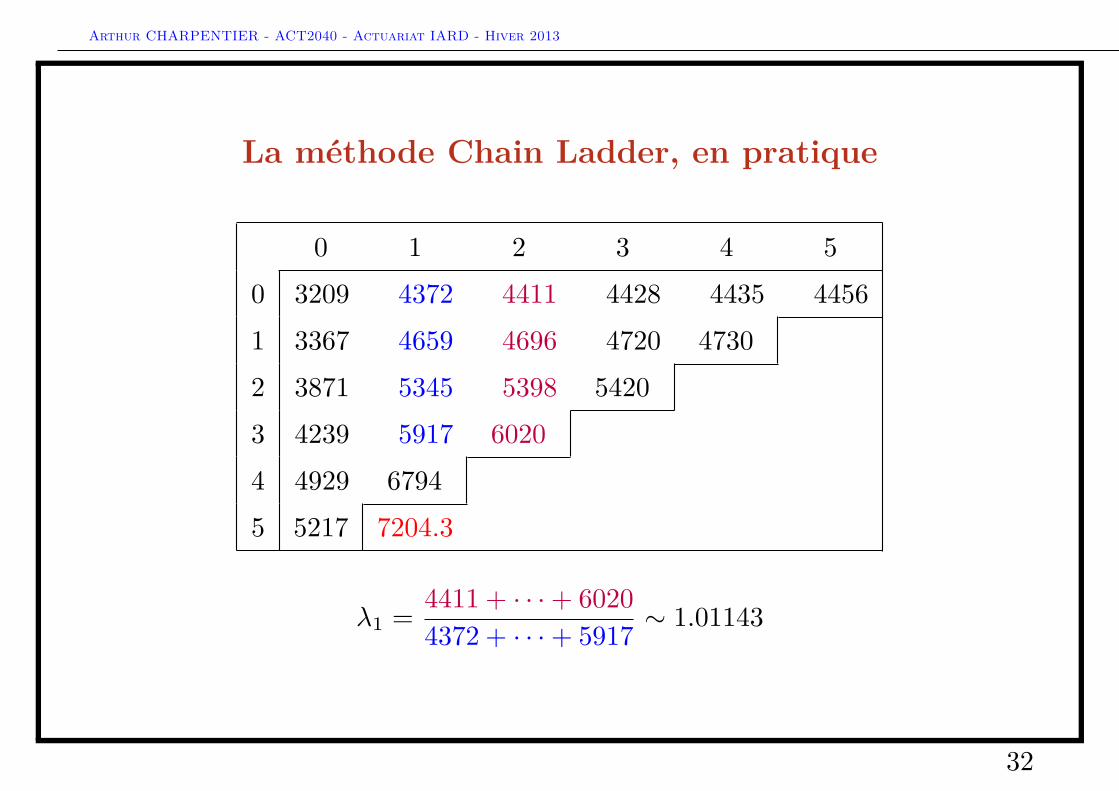
La méthode Chain Ladder, en pratique
0 1 2 3 4 50 3209 4372 4411 4428 4435 44561 3367 4659 4696 4720 4730 4752.42 3871 5345 5398 5420 5430.1 5455.83 4239 5917 6020 6046.1 6057.4 6086.14 4929 6794 6871.7 6901.5 6914.3 6947.15 5217 7204.3 7286.7 7318.3 7331.9 7366.7
λ1 = 4411 + · · ·+ 60204372 + · · ·+ 5917 ∼ 1.01143
32
Arthur CHARPENTIER - ACT2040 - Actuariat IARD - Hiver 2013
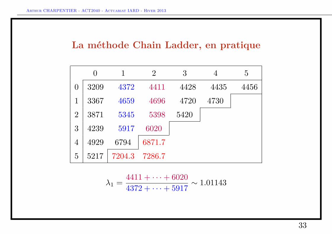
La méthode Chain Ladder, en pratique
0 1 2 3 4 50 3209 4372 4411 4428 4435 44561 3367 4659 4696 4720 4730 4752.42 3871 5345 5398 5420 5430.1 5455.83 4239 5917 6020 6046.1 6057.4 6086.14 4929 6794 6871.7 6901.5 6914.3 6947.15 5217 7204.3 7286.7 7318.3 7331.9 7366.7
λ1 = 4411 + · · ·+ 60204372 + · · ·+ 5917 ∼ 1.01143
33

Arthur CHARPENTIER - ACT2040 - Actuariat IARD - Hiver 2013
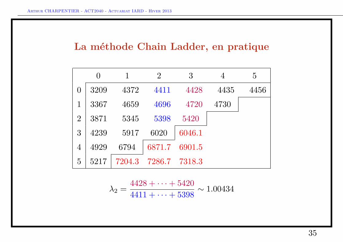
La méthode Chain Ladder, en pratique
0 1 2 3 4 50 3209 4372 4411 4428 4435 44561 3367 4659 4696 4720 4730 4752.42 3871 5345 5398 5420 5430.1 5455.83 4239 5917 6020 6046.1 6057.4 6086.14 4929 6794 6871.7 6901.5 6914.3 6947.15 5217 7204.3 7286.7 7318.3 7331.9 7366.7
λ2 = 4428 + · · ·+ 54204411 + · · ·+ 5398 ∼ 1.00434
34
Arthur CHARPENTIER - ACT2040 - Actuariat IARD - Hiver 2013
La méthode Chain Ladder, en pratique
0 1 2 3 4 50 3209 4372 4411 4428 4435 44561 3367 4659 4696 4720 4730 4752.42 3871 5345 5398 5420 5430.1 5455.83 4239 5917 6020 6046.1 6057.4 6086.14 4929 6794 6871.7 6901.5 6914.3 6947.15 5217 7204.3 7286.7 7318.3 7331.9 7366.7
λ2 = 4428 + · · ·+ 54204411 + · · ·+ 5398 ∼ 1.00434
35
Arthur CHARPENTIER - ACT2040 - Actuariat IARD - Hiver 2013
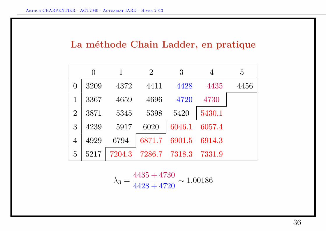
La méthode Chain Ladder, en pratique
0 1 2 3 4 50 3209 4372 4411 4428 4435 44561 3367 4659 4696 4720 4730 4752.42 3871 5345 5398 5420 5430.1 5455.83 4239 5917 6020 6046.1 6057.4 6086.14 4929 6794 6871.7 6901.5 6914.3 6947.15 5217 7204.3 7286.7 7318.3 7331.9 7366.7
λ3 = 4435 + 47304428 + 4720 ∼ 1.00186
36
Arthur CHARPENTIER - ACT2040 - Actuariat IARD - Hiver 2013
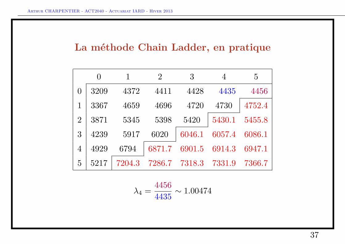
La méthode Chain Ladder, en pratique
0 1 2 3 4 50 3209 4372 4411 4428 4435 44561 3367 4659 4696 4720 4730 4752.42 3871 5345 5398 5420 5430.1 5455.83 4239 5917 6020 6046.1 6057.4 6086.14 4929 6794 6871.7 6901.5 6914.3 6947.15 5217 7204.3 7286.7 7318.3 7331.9 7366.7
λ4 = 44564435 ∼ 1.00474
37
Arthur CHARPENTIER - ACT2040 - Actuariat IARD - Hiver 2013
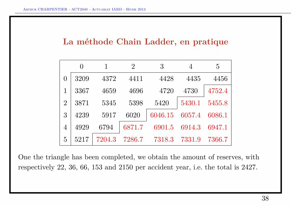
La méthode Chain Ladder, en pratique
0 1 2 3 4 50 3209 4372 4411 4428 4435 44561 3367 4659 4696 4720 4730 4752.42 3871 5345 5398 5420 5430.1 5455.83 4239 5917 6020 6046.15 6057.4 6086.14 4929 6794 6871.7 6901.5 6914.3 6947.15 5217 7204.3 7286.7 7318.3 7331.9 7366.7
One the triangle has been completed, we obtain the amount of reserves, withrespectively 22, 36, 66, 153 and 2150 per accident year, i.e. the total is 2427.
38
Arthur CHARPENTIER - ACT2040 - Actuariat IARD - Hiver 2013
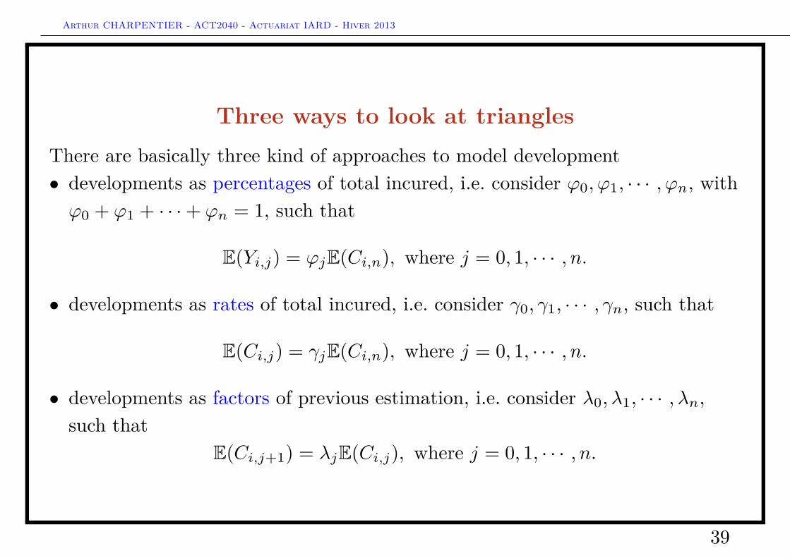
Three ways to look at trianglesThere are basically three kind of approaches to model development• developments as percentages of total incured, i.e. consider ϕ0, ϕ1, · · · , ϕn, withϕ0 + ϕ1 + · · ·+ ϕn = 1, such that
E(Yi,j) = ϕjE(Ci,n), where j = 0, 1, · · · , n.
• developments as rates of total incured, i.e. consider γ0, γ1, · · · , γn, such that
E(Ci,j) = γjE(Ci,n), where j = 0, 1, · · · , n.
• developments as factors of previous estimation, i.e. consider λ0, λ1, · · · , λn,such that
E(Ci,j+1) = λjE(Ci,j), where j = 0, 1, · · · , n.
39
Arthur CHARPENTIER - ACT2040 - Actuariat IARD - Hiver 2013
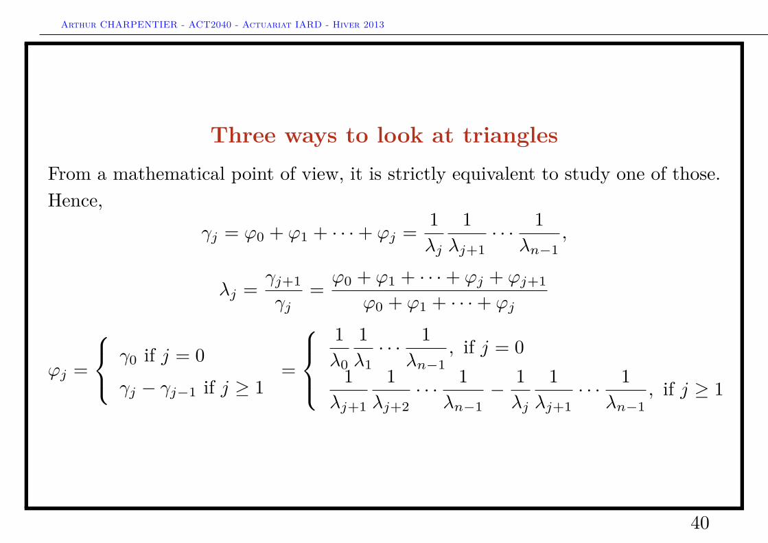
Three ways to look at trianglesFrom a mathematical point of view, it is strictly equivalent to study one of those.Hence,
γj = ϕ0 + ϕ1 + · · ·+ ϕj = 1λj
1λj+1
· · · 1λn−1
,
λj = γj+1
γj= ϕ0 + ϕ1 + · · ·+ ϕj + ϕj+1
ϕ0 + ϕ1 + · · ·+ ϕj
ϕj =
γ0 if j = 0γj − γj−1 if j ≥ 1
=
1λ0
1λ1· · · 1
λn−1, if j = 0
1λj+1
1λj+2
· · · 1λn−1
− 1λj
1λj+1
· · · 1λn−1
, if j ≥ 1
40
Arthur CHARPENTIER - ACT2040 - Actuariat IARD - Hiver 2013
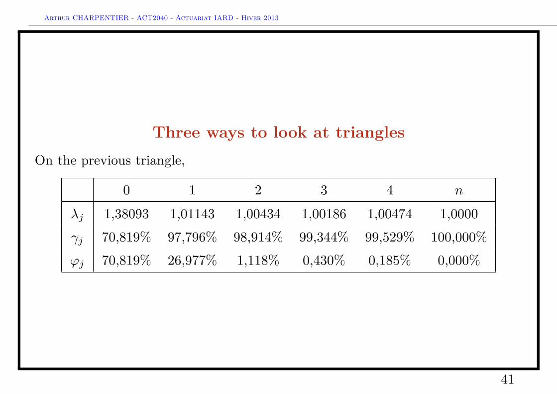
Three ways to look at trianglesOn the previous triangle,
0 1 2 3 4 n
λj 1,38093 1,01143 1,00434 1,00186 1,00474 1,0000γj 70,819% 97,796% 98,914% 99,344% 99,529% 100,000%ϕj 70,819% 26,977% 1,118% 0,430% 0,185% 0,000%
41
Arthur CHARPENTIER - ACT2040 - Actuariat IARD - Hiver 2013
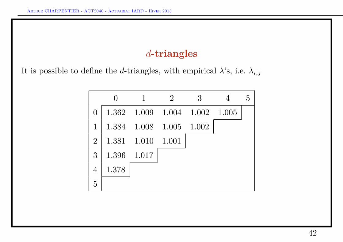
d-trianglesIt is possible to define the d-triangles, with empirical λ’s, i.e. λi,j
0 1 2 3 4 50 1.362 1.009 1.004 1.002 1.0051 1.384 1.008 1.005 1.0022 1.381 1.010 1.0013 1.396 1.0174 1.3785
42
Arthur CHARPENTIER - ACT2040 - Actuariat IARD - Hiver 2013
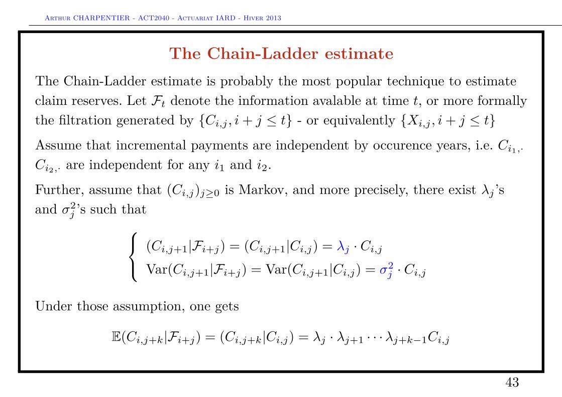
The Chain-Ladder estimateThe Chain-Ladder estimate is probably the most popular technique to estimateclaim reserves. Let Ft denote the information avalable at time t, or more formallythe filtration generated by {Ci,j , i+ j ≤ t} - or equivalently {Xi,j , i+ j ≤ t}
Assume that incremental payments are independent by occurence years, i.e. Ci1,·Ci2,· are independent for any i1 and i2.
Further, assume that (Ci,j)j≥0 is Markov, and more precisely, there exist λj ’sand σ2
j ’s such that (Ci,j+1|Fi+j) = (Ci,j+1|Ci,j) = λj · Ci,jVar(Ci,j+1|Fi+j) = Var(Ci,j+1|Ci,j) = σ2
j · Ci,j
Under those assumption, one gets
E(Ci,j+k|Fi+j) = (Ci,j+k|Ci,j) = λj · λj+1 · · ·λj+k−1Ci,j
43
Arthur CHARPENTIER - ACT2040 - Actuariat IARD - Hiver 2013
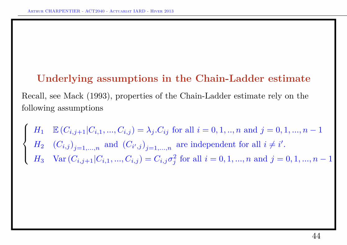
Underlying assumptions in the Chain-Ladder estimateRecall, see Mack (1993), properties of the Chain-Ladder estimate rely on thefollowing assumptions
H1 E (Ci,j+1|Ci,1, ..., Ci,j) = λj .Cij for all i = 0, 1, .., n and j = 0, 1, ..., n− 1H2 (Ci,j)j=1,...,n and (Ci′,j)j=1,...,n are independent for all i 6= i′.
H3 Var (Ci,j+1|Ci,1, ..., Ci,j) = Ci,jσ2j for all i = 0, 1, ..., n and j = 0, 1, ..., n− 1
44
Arthur CHARPENTIER - ACT2040 - Actuariat IARD - Hiver 2013
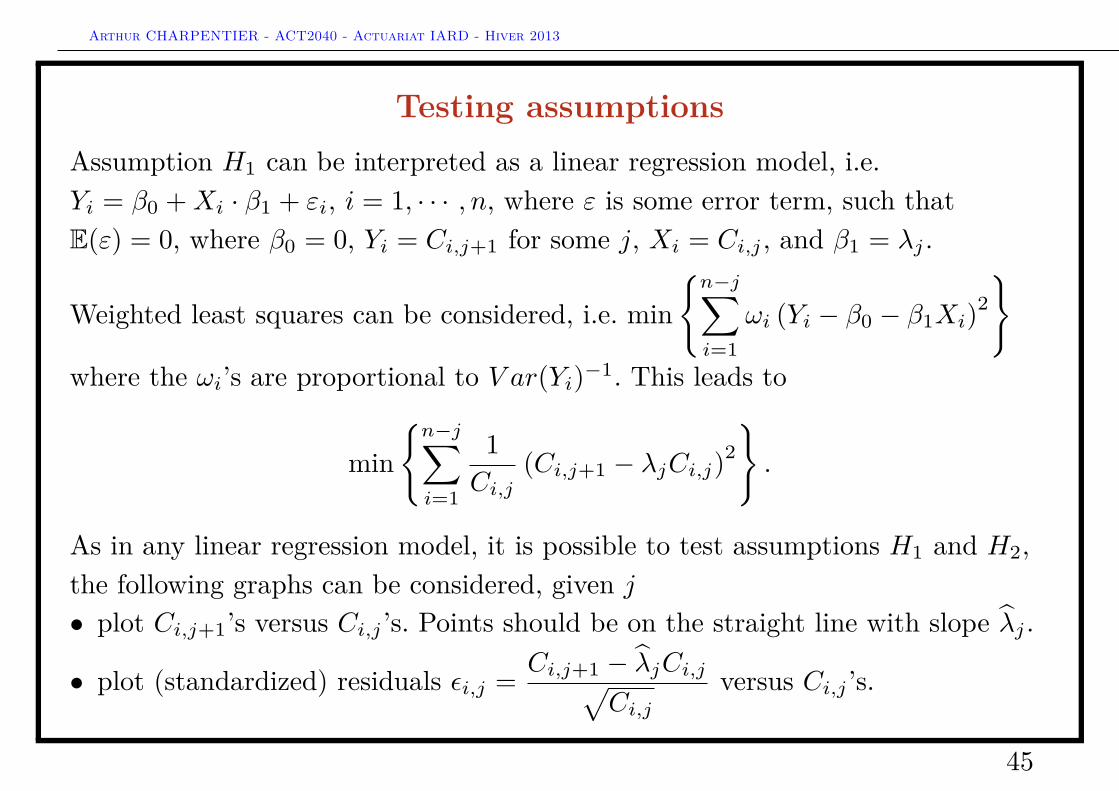
Testing assumptionsAssumption H1 can be interpreted as a linear regression model, i.e.Yi = β0 +Xi · β1 + εi, i = 1, · · · , n, where ε is some error term, such thatE(ε) = 0, where β0 = 0, Yi = Ci,j+1 for some j, Xi = Ci,j , and β1 = λj .
Weighted least squares can be considered, i.e. min{n−j∑i=1
ωi (Yi − β0 − β1Xi)2
}where the ωi’s are proportional to V ar(Yi)−1. This leads to
min{n−j∑i=1
1Ci,j
(Ci,j+1 − λjCi,j)2
}.
As in any linear regression model, it is possible to test assumptions H1 and H2,the following graphs can be considered, given j• plot Ci,j+1’s versus Ci,j ’s. Points should be on the straight line with slope λj .
• plot (standardized) residuals εi,j = Ci,j+1 − λjCi,j√Ci,j
versus Ci,j ’s.
45
Arthur CHARPENTIER - ACT2040 - Actuariat IARD - Hiver 2013
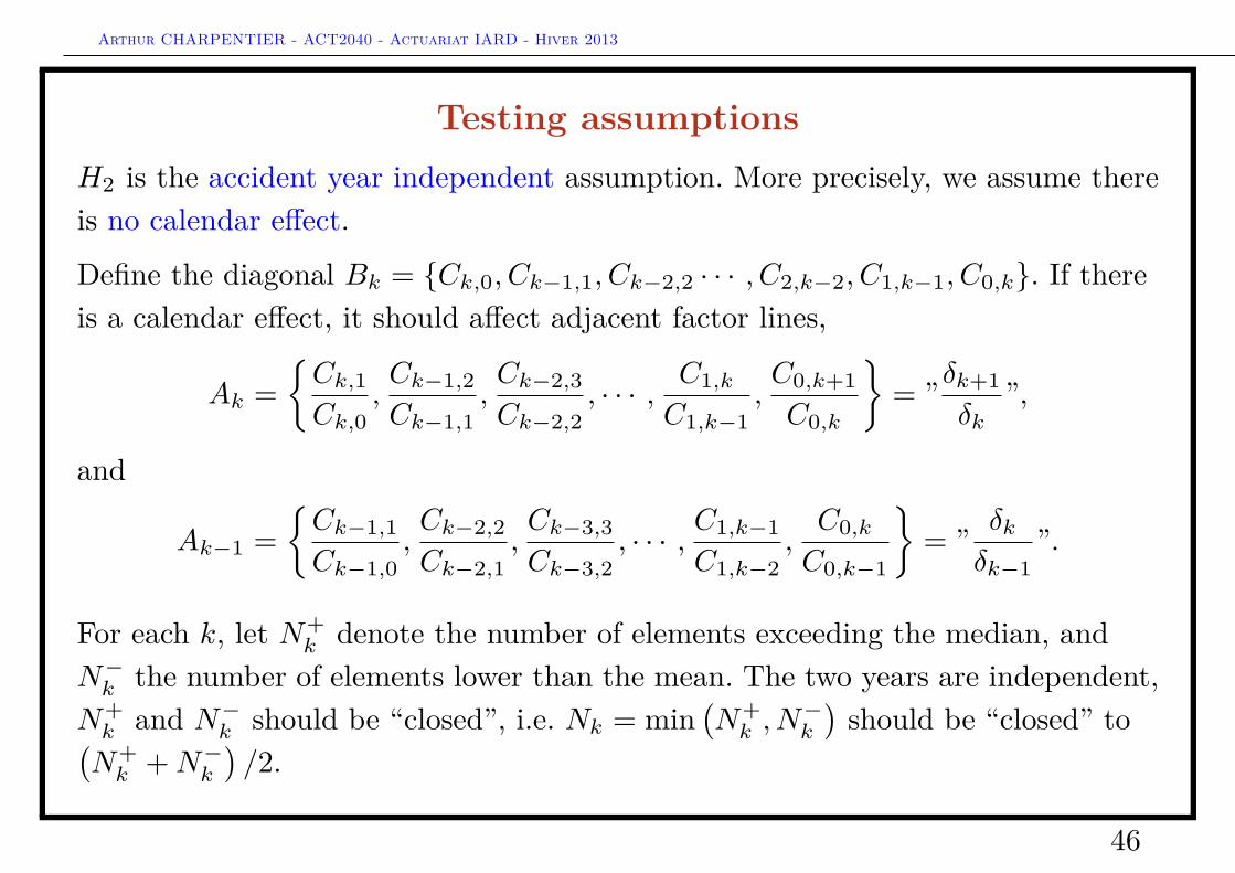
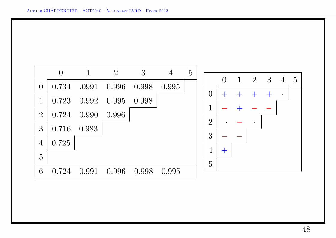
Testing assumptionsH2 is the accident year independent assumption. More precisely, we assume thereis no calendar effect.
Define the diagonal Bk = {Ck,0, Ck−1,1, Ck−2,2 · · · , C2,k−2, C1,k−1, C0,k}. If thereis a calendar effect, it should affect adjacent factor lines,
Ak ={Ck,1Ck,0
,Ck−1,2
Ck−1,1,Ck−2,3
Ck−2,2, · · · , C1,k
C1,k−1,C0,k+1
C0,k
}= ”δk+1
δk”,
and
Ak−1 ={Ck−1,1
Ck−1,0,Ck−2,2
Ck−2,1,Ck−3,3
Ck−3,2, · · · , C1,k−1
C1,k−2,C0,k
C0,k−1
}= ” δk
δk−1”.
For each k, let N+k denote the number of elements exceeding the median, and
N−k the number of elements lower than the mean. The two years are independent,N+k and N−k should be “closed”, i.e. Nk = min
(N+k , N
−k
)should be “closed” to(
N+k +N−k
)/2.
46
Arthur CHARPENTIER - ACT2040 - Actuariat IARD - Hiver 2013
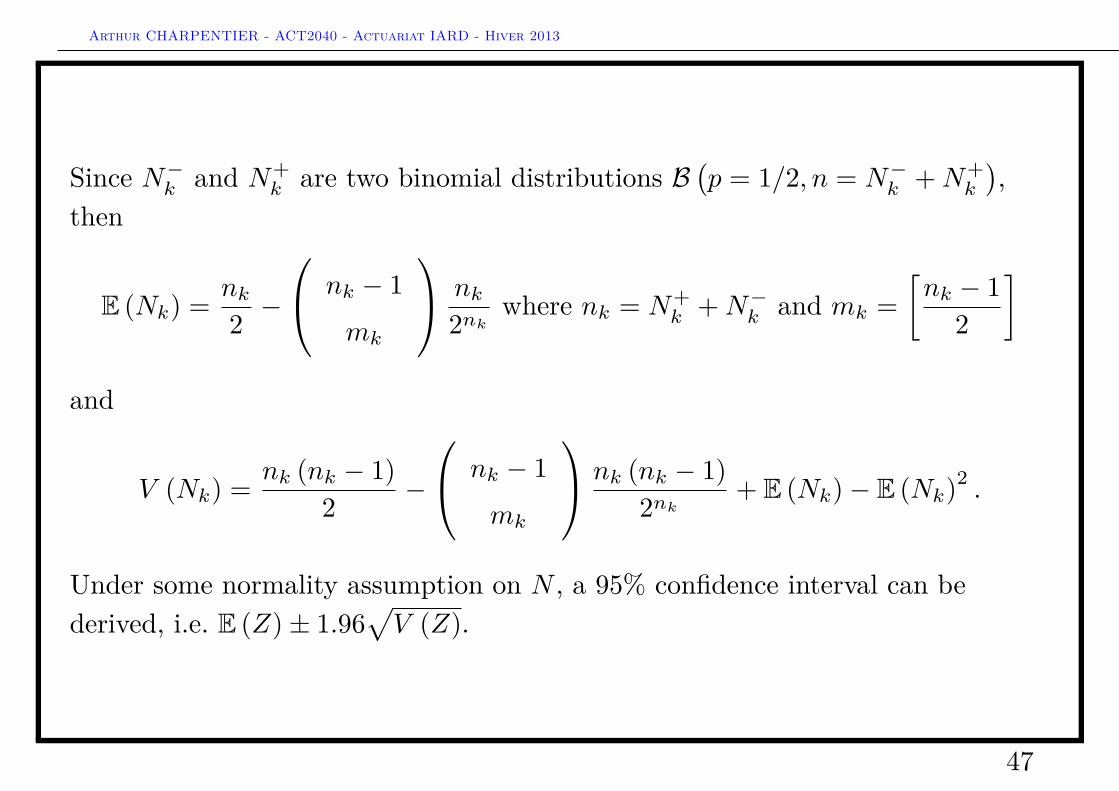
Since N−k and N+k are two binomial distributions B
(p = 1/2, n = N−k +N+
k
),
then
E (Nk) = nk2 −
nk − 1mk
nk2nk
where nk = N+k +N−k and mk =
[nk − 1
2
]
and
V (Nk) = nk (nk − 1)2 −
nk − 1mk
nk (nk − 1)2nk
+ E (Nk)− E (Nk)2.
Under some normality assumption on N , a 95% confidence interval can bederived, i.e. E (Z)± 1.96
√V (Z).
47
Arthur CHARPENTIER - ACT2040 - Actuariat IARD - Hiver 2013
0 1 2 3 4 50 0.734 .0991 0.996 0.998 0.9951 0.723 0.992 0.995 0.9982 0.724 0.990 0.9963 0.716 0.9834 0.7255
6 0.724 0.991 0.996 0.998 0.995
et
0 1 2 3 4 50 + + + + ·1 − + − −2 · − ·3 − −4 +5
48
Arthur CHARPENTIER - ACT2040 - Actuariat IARD - Hiver 2013
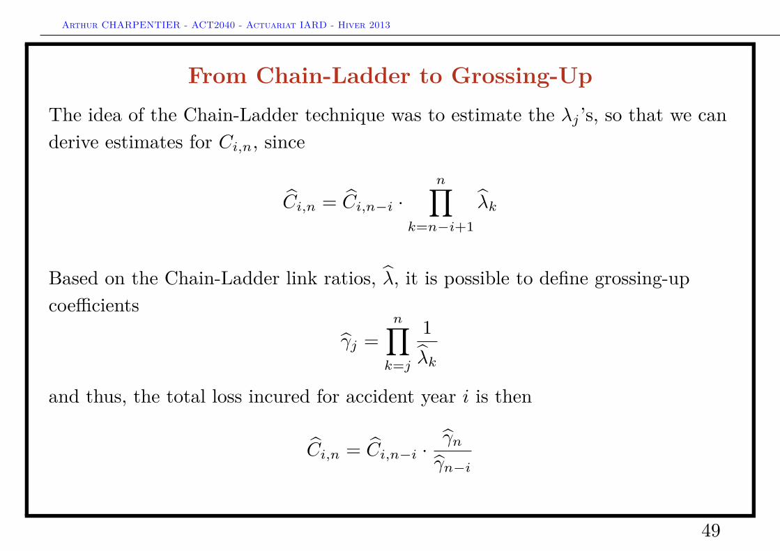
From Chain-Ladder to Grossing-UpThe idea of the Chain-Ladder technique was to estimate the λj ’s, so that we canderive estimates for Ci,n, since
Ci,n = Ci,n−i ·n∏
k=n−i+1λk
Based on the Chain-Ladder link ratios, λ, it is possible to define grossing-upcoefficients
γj =n∏k=j
1λk
and thus, the total loss incured for accident year i is then
Ci,n = Ci,n−i ·γnγn−i
49
Arthur CHARPENTIER - ACT2040 - Actuariat IARD - Hiver 2013
Variant of the Chain-Ladder Method (1)Historically (see e.g.), the natural idea was to consider a (standard) average ofindividual link ratios.
Several techniques have been introduces to study individual link-ratios.
A first idea is to consider a simple linear model, λi,j = aji+ bj . Using OLStechniques, it is possible to estimate those coefficients simply. Then, we projectthose ratios using predicted one, λi,j = aji+ bj .
50

Arthur CHARPENTIER - ACT2040 - Actuariat IARD - Hiver 2013
Variant of the Chain-Ladder Method (2)A second idea is to assume that λj is the weighted sum of λ··· ,j ’s,
λj =∑j−1i=0 ωi,jλi,j∑j−1i=0 ωi,j
If ωi,j = Ci,j we obtain the chain ladder estimate. An alternative is to assumethat ωi,j = i+ j + 1 (in order to give more weight to recent years).
51
Arthur CHARPENTIER - ACT2040 - Actuariat IARD - Hiver 2013
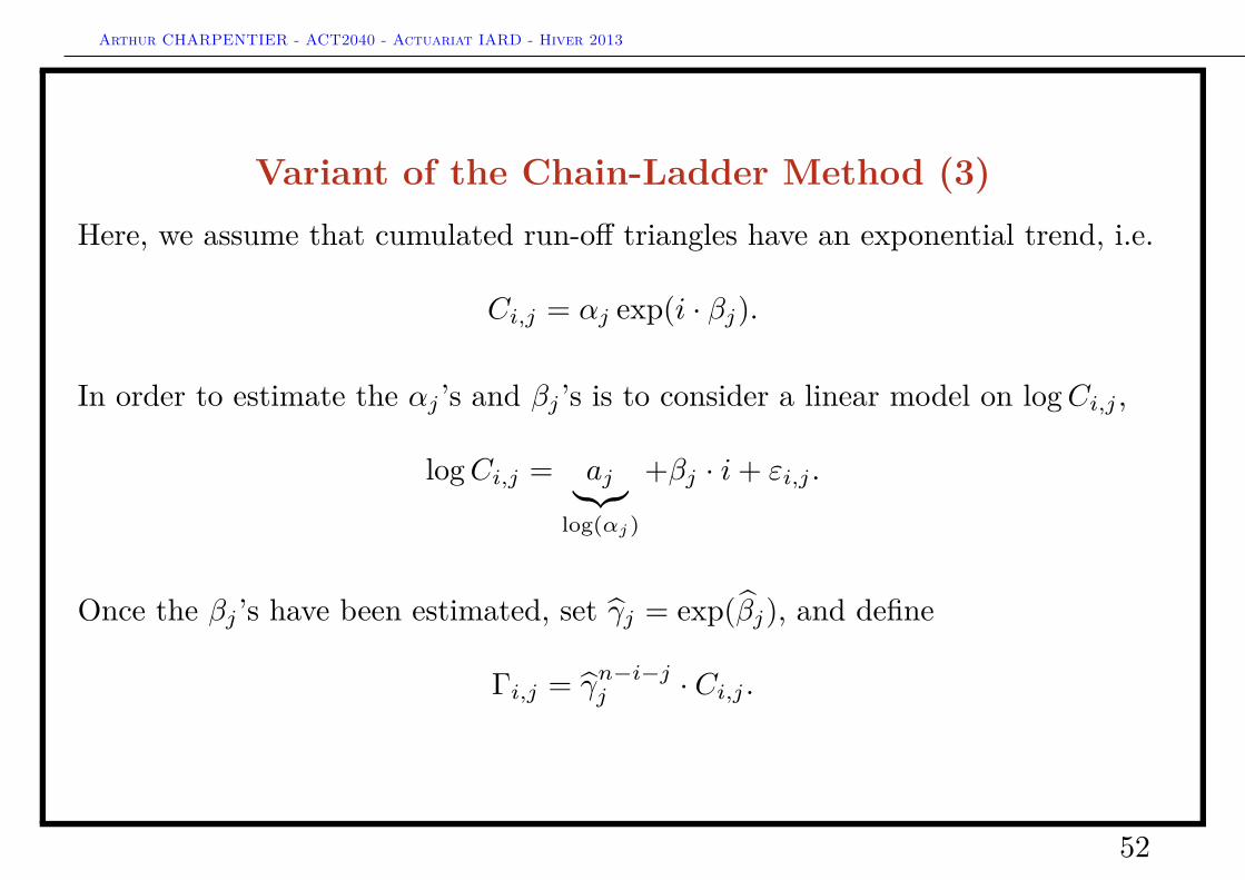
Variant of the Chain-Ladder Method (3)Here, we assume that cumulated run-off triangles have an exponential trend, i.e.
Ci,j = αj exp(i · βj).
In order to estimate the αj ’s and βj ’s is to consider a linear model on logCi,j ,
logCi,j = aj︸︷︷︸log(αj)
+βj · i+ εi,j .
Once the βj ’s have been estimated, set γj = exp(βj), and define
Γi,j = γn−i−jj · Ci,j .
52
Arthur CHARPENTIER - ACT2040 - Actuariat IARD - Hiver 2013
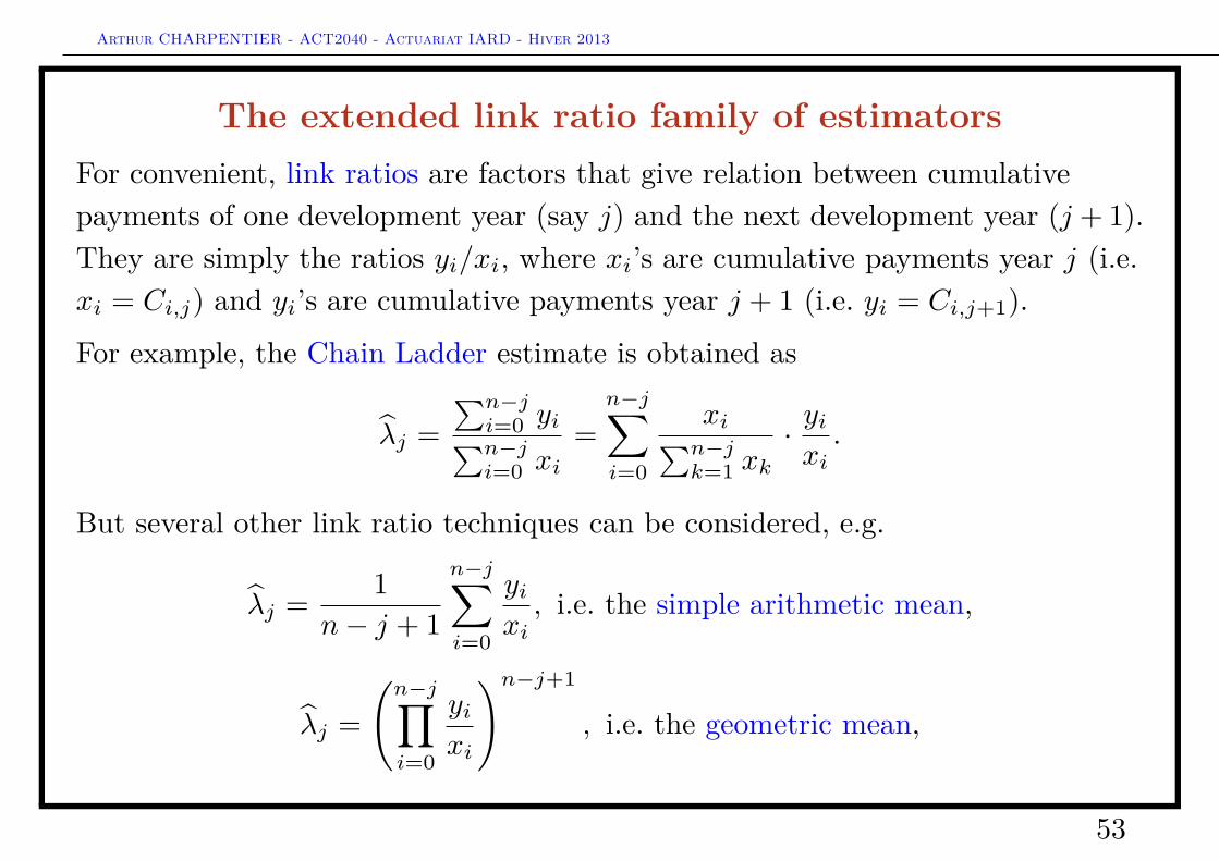
The extended link ratio family of estimatorsFor convenient, link ratios are factors that give relation between cumulativepayments of one development year (say j) and the next development year (j + 1).They are simply the ratios yi/xi, where xi’s are cumulative payments year j (i.e.xi = Ci,j) and yi’s are cumulative payments year j + 1 (i.e. yi = Ci,j+1).
For example, the Chain Ladder estimate is obtained as
λj =∑n−ji=0 yi∑n−ji=0 xi
=n−j∑i=0
xi∑n−jk=1 xk
· yixi.
But several other link ratio techniques can be considered, e.g.
λj = 1n− j + 1
n−j∑i=0
yixi, i.e. the simple arithmetic mean,
λj =(n−j∏i=0
yixi
)n−j+1
, i.e. the geometric mean,
53
Arthur CHARPENTIER - ACT2040 - Actuariat IARD - Hiver 2013
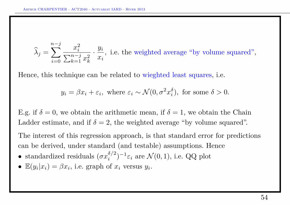
λj =n−j∑i=0
x2i∑n−j
k=1 x2k
· yixi, i.e. the weighted average “by volume squared”,
Hence, this technique can be related to wieghted least squares, i.e.
yi = βxi + εi, where εi ∼ N (0, σ2xδi ), for some δ > 0.
E.g. if δ = 0, we obtain the arithmetic mean, if δ = 1, we obtain the ChainLadder estimate, and if δ = 2, the weighted average “by volume squared”.
The interest of this regression approach, is that standard error for predictionscan be derived, under standard (and testable) assumptions. Hence• standardized residuals (σxδ/2
i )−1εi are N (0, 1), i.e. QQ plot• E(yi|xi) = βxi, i.e. graph of xi versus yi.
54
Arthur CHARPENTIER - ACT2040 - Actuariat IARD - Hiver 2013
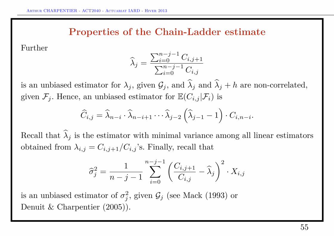
Properties of the Chain-Ladder estimateFurther
λj =∑n−j−1i=0 Ci,j+1∑n−j−1i=0 Ci,j
is an unbiased estimator for λj , given Gj , and λj and λj + h are non-correlated,given Fj . Hence, an unbiased estimator for E(Ci,j |Fi) is
Ci,j = λn−i · λn−i+1 · · · λj−2
(λj−1 − 1
)· Ci,n−i.
Recall that λj is the estimator with minimal variance among all linear estimatorsobtained from λi,j = Ci,j+1/Ci,j ’s. Finally, recall that
σ2j = 1
n− j − 1
n−j−1∑i=0
(Ci,j+1
Ci,j− λj
)2·Xi,j
is an unbiased estimator of σ2j , given Gj (see Mack (1993) or
Denuit & Charpentier (2005)).
55
Arthur CHARPENTIER - ACT2040 - Actuariat IARD - Hiver 2013
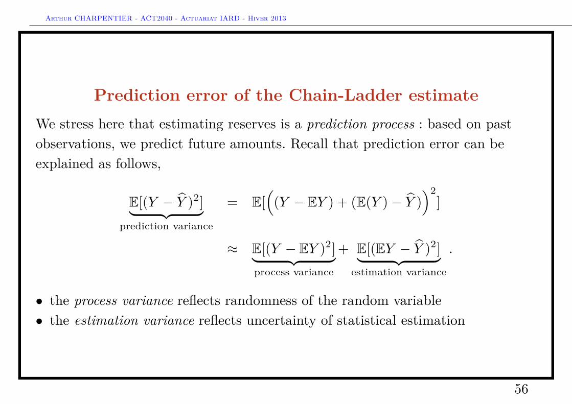
Prediction error of the Chain-Ladder estimateWe stress here that estimating reserves is a prediction process : based on pastobservations, we predict future amounts. Recall that prediction error can beexplained as follows,
E[(Y − Y )2]︸ ︷︷ ︸prediction variance
= E[(
(Y − EY ) + (E(Y )− Y ))2
]
≈ E[(Y − EY )2]︸ ︷︷ ︸process variance
+ E[(EY − Y )2]︸ ︷︷ ︸estimation variance
.
• the process variance reflects randomness of the random variable• the estimation variance reflects uncertainty of statistical estimation
56
Arthur CHARPENTIER - ACT2040 - Actuariat IARD - Hiver 2013
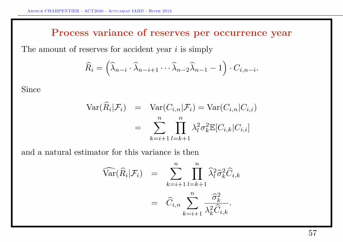
Process variance of reserves per occurrence yearThe amount of reserves for accident year i is simply
Ri =(λn−i · λn−i+1 · · · λn−2λn−1 − 1
)· Ci,n−i.
Since
Var(Ri|Fi) = Var(Ci,n|Fi) = Var(Ci,n|Ci,i)
=n∑
k=i+1
n∏l=k+1
λ2l σ
2kE[Ci,k|Ci,i]
and a natural estimator for this variance is then
Var(Ri|Fi) =n∑
k=i+1
n∏l=k+1
λ2l σ
2kCi,k
= Ci,n
n∑k=i+1
σ2k
λ2kCi,k
.
57
Arthur CHARPENTIER - ACT2040 - Actuariat IARD - Hiver 2013
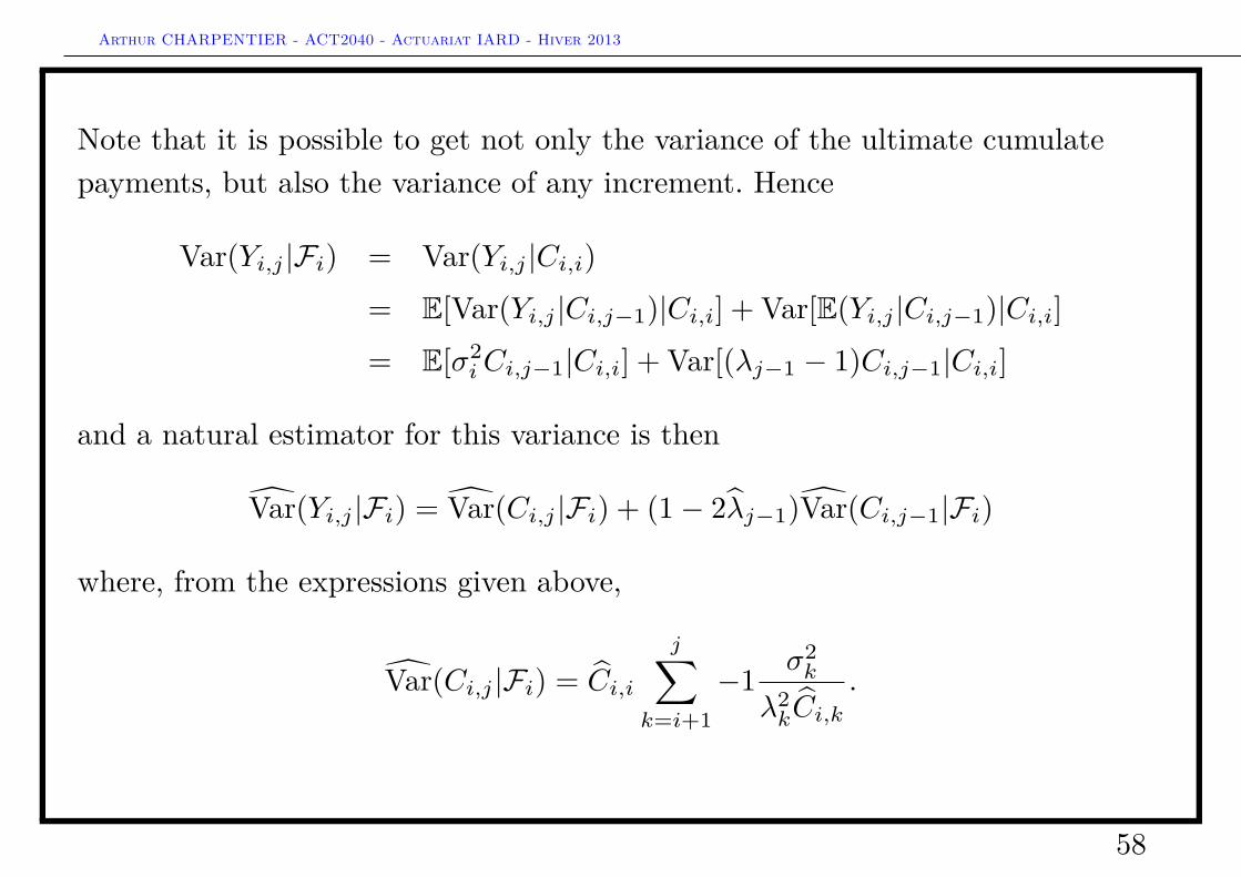
Note that it is possible to get not only the variance of the ultimate cumulatepayments, but also the variance of any increment. Hence
Var(Yi,j |Fi) = Var(Yi,j |Ci,i)= E[Var(Yi,j |Ci,j−1)|Ci,i] + Var[E(Yi,j |Ci,j−1)|Ci,i]= E[σ2
iCi,j−1|Ci,i] + Var[(λj−1 − 1)Ci,j−1|Ci,i]
and a natural estimator for this variance is then
Var(Yi,j |Fi) = Var(Ci,j |Fi) + (1− 2λj−1)Var(Ci,j−1|Fi)
where, from the expressions given above,
Var(Ci,j |Fi) = Ci,i
j∑k=i+1
−1 σ2k
λ2kCi,k
.
58

Arthur CHARPENTIER - ACT2040 - Actuariat IARD - Hiver 2013
Parameter variance when estimating reserves peroccurrence year
So far, we have obtained an estimate for the process error of technical risks(increments or cumulated payments). But since parameters λj ’s and σ2
j areestimated from past information, there is an additional potential error, alsocalled parameter error (or estimation error). Hence, we have to quantifyE(
[Ri − Ri]2). In order to quantify that error, Murphy (1994) assume the
following underlying model,
Ci,j = λj−1Ci,j−1 + ηi,j (1)
with independent variables ηi,j . From the structure of the conditional variance,
Var(Ci,j+1|Fi+j) = Var(Ci,j+1|Ci,j) = σ2j · Ci,j ,
it is natural to write Equation (1) as
Ci,j = λj−1Ci,j−1 + σj−1√Ci,j−1εi,j , (2)
59
Arthur CHARPENTIER - ACT2040 - Actuariat IARD - Hiver 2013
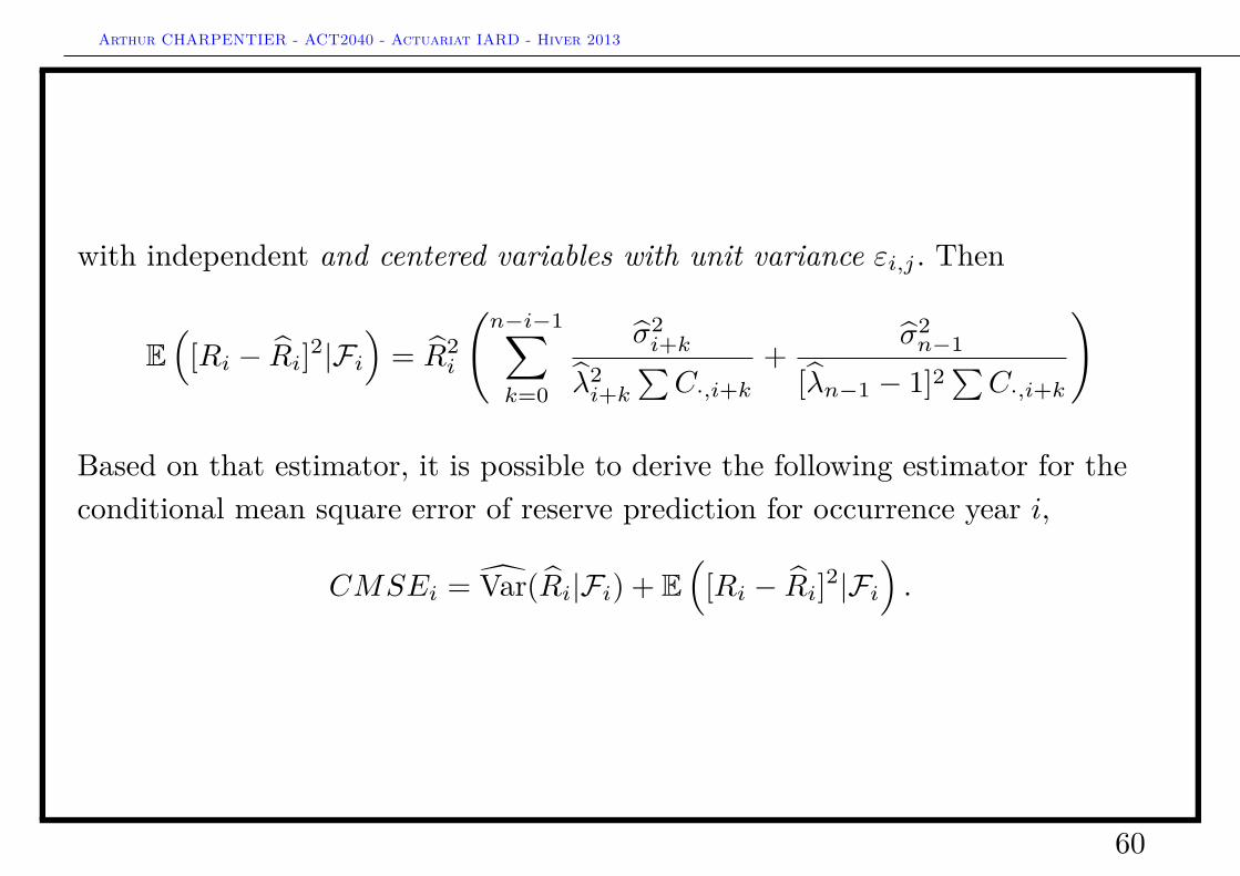
with independent and centered variables with unit variance εi,j . Then
E(
[Ri − Ri]2|Fi)
= R2i
(n−i−1∑k=0
σ2i+k
λ2i+k∑C·,i+k
+σ2n−1
[λn−1 − 1]2∑C·,i+k
)
Based on that estimator, it is possible to derive the following estimator for theconditional mean square error of reserve prediction for occurrence year i,
CMSEi = Var(Ri|Fi) + E(
[Ri − Ri]2|Fi).
60
Arthur CHARPENTIER - ACT2040 - Actuariat IARD - Hiver 2013
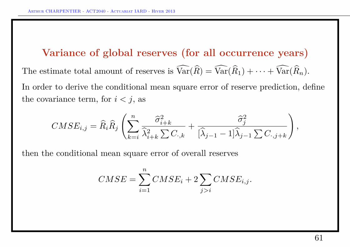
Variance of global reserves (for all occurrence years)
The estimate total amount of reserves is Var(R) = Var(R1) + · · ·+ Var(Rn).
In order to derive the conditional mean square error of reserve prediction, definethe covariance term, for i < j, as
CMSEi,j = RiRj
(n∑k=i
σ2i+k
λ2i+k∑C·,k
+σ2j
[λj−1 − 1]λj−1∑C·,j+k
),
then the conditional mean square error of overall reserves
CMSE =n∑i=1
CMSEi + 2∑j>i
CMSEi,j .
61
Arthur CHARPENTIER - ACT2040 - Actuariat IARD - Hiver 2013
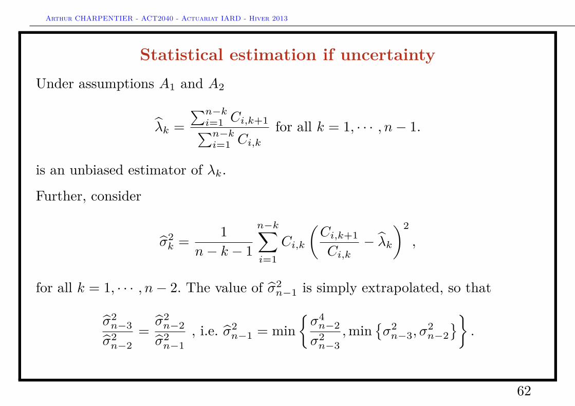
Statistical estimation if uncertaintyUnder assumptions A1 and A2
λk =∑n−ki=1 Ci,k+1∑n−ki=1 Ci,k
for all k = 1, · · · , n− 1.
is an unbiased estimator of λk.
Further, consider
σ2k = 1
n− k − 1
n−k∑i=1
Ci,k
(Ci,k+1
Ci,k− λk
)2,
for all k = 1, · · · , n− 2. The value of σ2n−1 is simply extrapolated, so that
σ2n−3σ2n−2
=σ2n−2σ2n−1
, i.e. σ2n−1 = min
{σ4n−2σ2n−3
,min{σ2n−3, σ
2n−2}}
.
62
Arthur CHARPENTIER - ACT2040 - Actuariat IARD - Hiver 2013
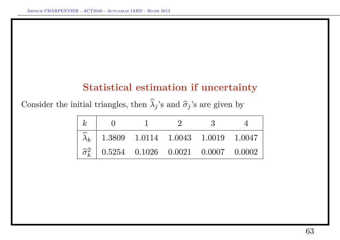
Statistical estimation if uncertaintyConsider the initial triangles, then λj ’s and σj ’s are given by
k 0 1 2 3 4
λk 1.3809 1.0114 1.0043 1.0019 1.0047σ2k 0.5254 0.1026 0.0021 0.0007 0.0002
63
Arthur CHARPENTIER - ACT2040 - Actuariat IARD - Hiver 2013
A short word on Munich Chain LadderMunich chain ladder is an extension of Mack’s technique based on paid (P ) andincurred (I) losses.
Here we adjust the chain-ladder link-ratios λj ’s depending if the momentary(P/I) ratio is above or below average. It integrated correlation of residualsbetween P vs. I/P and I vs. P/I chain-ladder link-ratio to estimate thecorrection factor.
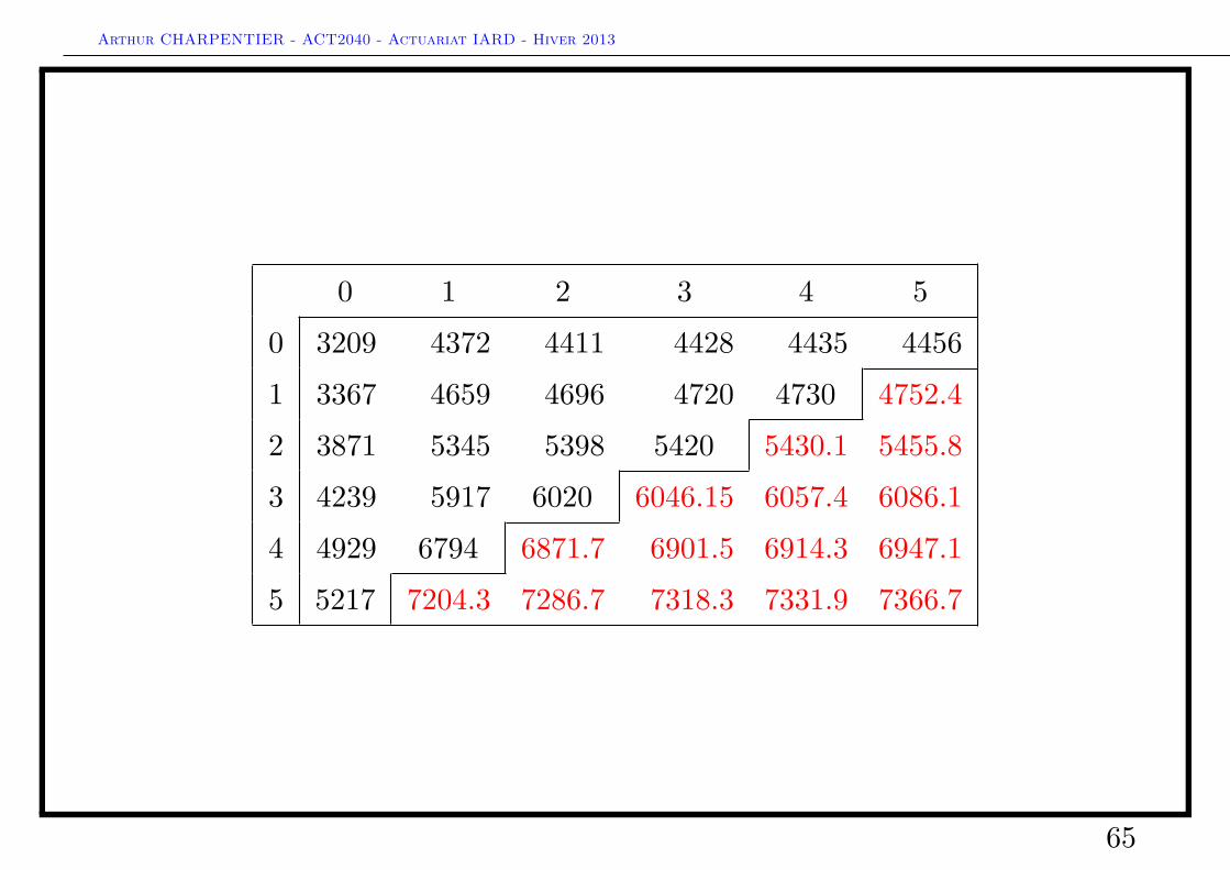
Use standard Chain Ladder technique on the two triangles,
64
Arthur CHARPENTIER - ACT2040 - Actuariat IARD - Hiver 2013
0 1 2 3 4 50 3209 4372 4411 4428 4435 44561 3367 4659 4696 4720 4730 4752.42 3871 5345 5398 5420 5430.1 5455.83 4239 5917 6020 6046.15 6057.4 6086.14 4929 6794 6871.7 6901.5 6914.3 6947.15 5217 7204.3 7286.7 7318.3 7331.9 7366.7
65
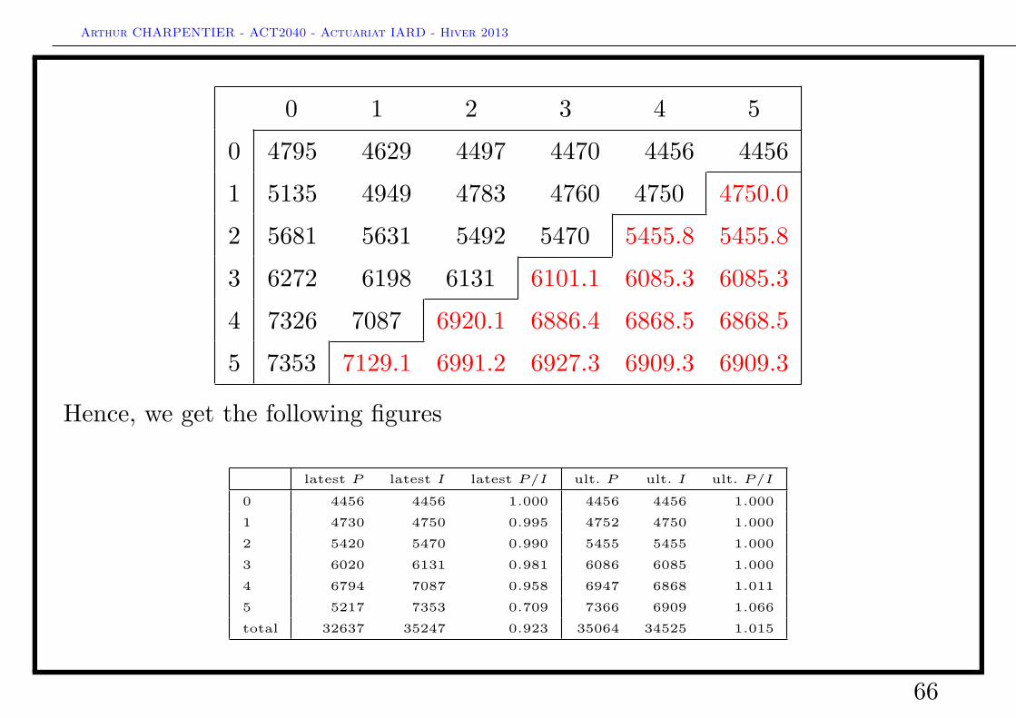
Arthur CHARPENTIER - ACT2040 - Actuariat IARD - Hiver 2013
0 1 2 3 4 50 4795 4629 4497 4470 4456 44561 5135 4949 4783 4760 4750 4750.02 5681 5631 5492 5470 5455.8 5455.83 6272 6198 6131 6101.1 6085.3 6085.34 7326 7087 6920.1 6886.4 6868.5 6868.55 7353 7129.1 6991.2 6927.3 6909.3 6909.3
Hence, we get the following figures
latest P latest I latest P/I ult. P ult. I ult. P/I
0 4456 4456 1.000 4456 4456 1.0001 4730 4750 0.995 4752 4750 1.0002 5420 5470 0.990 5455 5455 1.0003 6020 6131 0.981 6086 6085 1.0004 6794 7087 0.958 6947 6868 1.0115 5217 7353 0.709 7366 6909 1.066total 32637 35247 0.923 35064 34525 1.015
66
Arthur CHARPENTIER - ACT2040 - Actuariat IARD - Hiver 2013
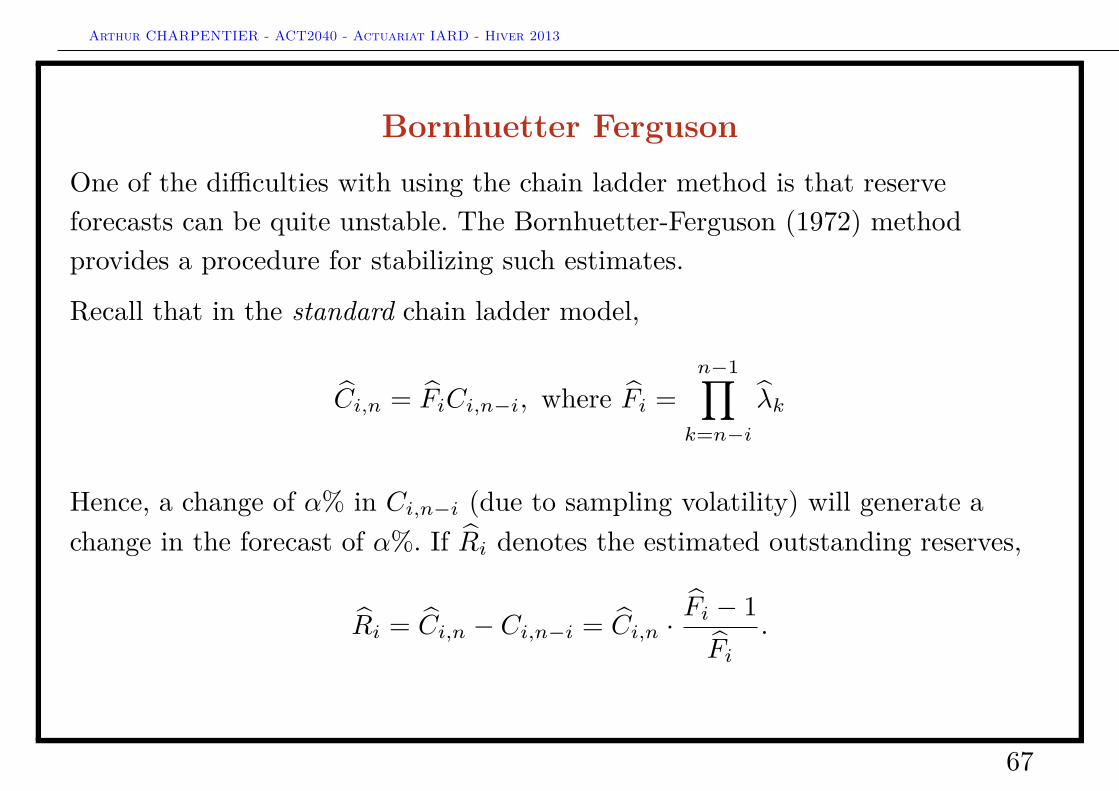
Bornhuetter FergusonOne of the difficulties with using the chain ladder method is that reserveforecasts can be quite unstable. The Bornhuetter-Ferguson (1972) methodprovides a procedure for stabilizing such estimates.
Recall that in the standard chain ladder model,
Ci,n = FiCi,n−i, where Fi =n−1∏k=n−i
λk
Hence, a change of α% in Ci,n−i (due to sampling volatility) will generate achange in the forecast of α%. If Ri denotes the estimated outstanding reserves,
Ri = Ci,n − Ci,n−i = Ci,n ·Fi − 1Fi
.
67
Arthur CHARPENTIER - ACT2040 - Actuariat IARD - Hiver 2013
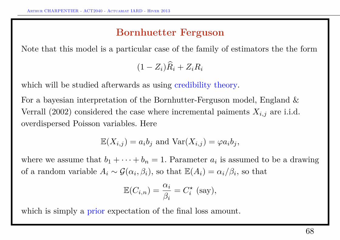
Bornhuetter FergusonNote that this model is a particular case of the family of estimators the the form
(1− Zi)Ri + ZiRi
which will be studied afterwards as using credibility theory.
For a bayesian interpretation of the Bornhutter-Ferguson model, England &Verrall (2002) considered the case where incremental paiments Xi,j are i.i.d.overdispersed Poisson variables. Here
E(Xi,j) = aibj and Var(Xi,j) = ϕaibj ,
where we assume that b1 + · · ·+ bn = 1. Parameter ai is assumed to be a drawingof a random variable Ai ∼ G(αi, βi), so that E(Ai) = αi/βi, so that
E(Ci,n) = αiβi
= C?i (say),
which is simply a prior expectation of the final loss amount.
68
Arthur CHARPENTIER - ACT2040 - Actuariat IARD - Hiver 2013
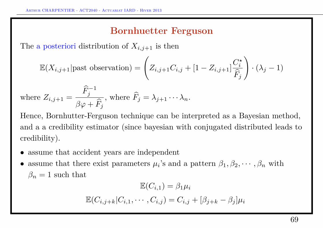
Bornhuetter FergusonThe a posteriori distribution of Xi,j+1 is then
E(Xi,j+1|past observation) =(Zi,j+1Ci,j + [1− Zi,j+1]C
?i
Fj
)· (λj − 1)
where Zi,j+1 =F−1j
βϕ+ Fj, where Fj = λj+1 · · ·λn.
Hence, Bornhutter-Ferguson technique can be interpreted as a Bayesian method,and a a credibility estimator (since bayesian with conjugated distributed leads tocredibility).
• assume that accident years are independent• assume that there exist parameters µi’s and a pattern β1, β2, · · · , βn withβn = 1 such that
E(Ci,1) = β1µi
E(Ci,j+k|Ci,1, · · · , Ci,j) = Ci,j + [βj+k − βj ]µi
69
Arthur CHARPENTIER - ACT2040 - Actuariat IARD - Hiver 2013
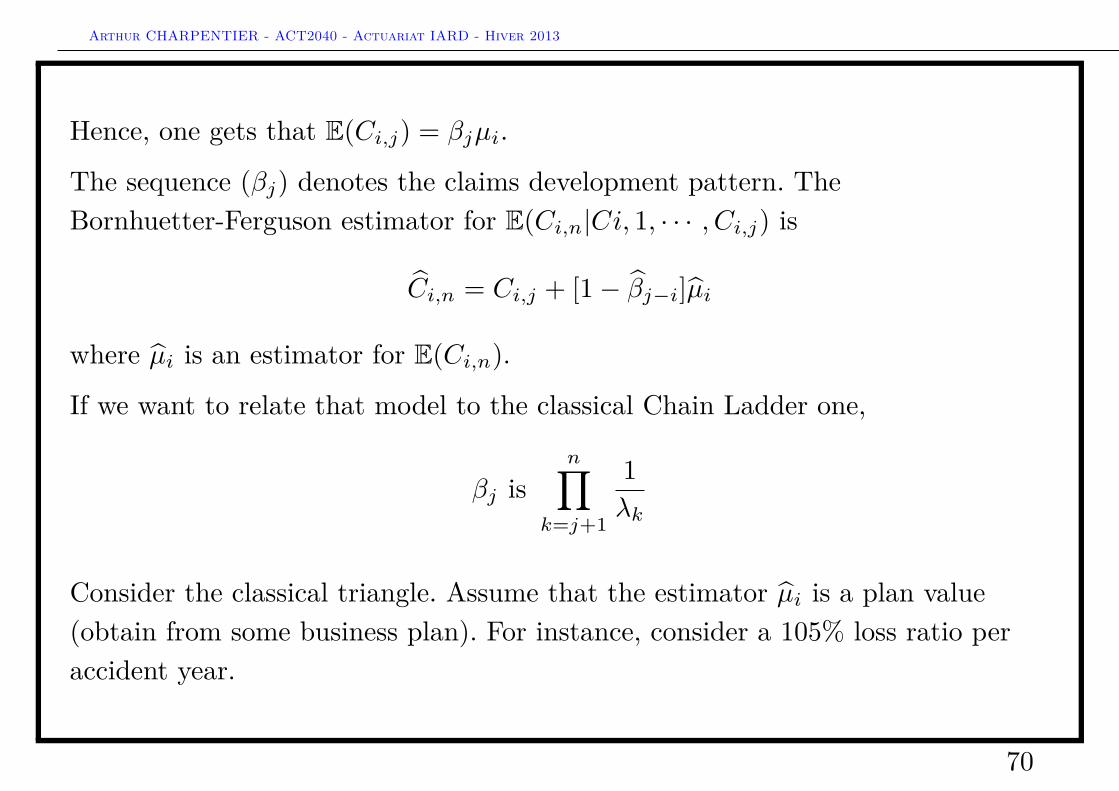
Hence, one gets that E(Ci,j) = βjµi.
The sequence (βj) denotes the claims development pattern. TheBornhuetter-Ferguson estimator for E(Ci,n|Ci, 1, · · · , Ci,j) is
Ci,n = Ci,j + [1− βj−i]µi
where µi is an estimator for E(Ci,n).
If we want to relate that model to the classical Chain Ladder one,
βj isn∏
k=j+1
1λk
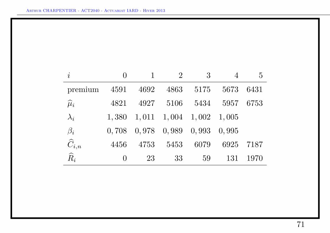
Consider the classical triangle. Assume that the estimator µi is a plan value(obtain from some business plan). For instance, consider a 105% loss ratio peraccident year.
70
Arthur CHARPENTIER - ACT2040 - Actuariat IARD - Hiver 2013
i 0 1 2 3 4 5
premium 4591 4692 4863 5175 5673 6431µi 4821 4927 5106 5434 5957 6753λi 1, 380 1, 011 1, 004 1, 002 1, 005βi 0, 708 0, 978 0, 989 0, 993 0, 995Ci,n 4456 4753 5453 6079 6925 7187Ri 0 23 33 59 131 1970
71
Arthur CHARPENTIER - ACT2040 - Actuariat IARD - Hiver 2013
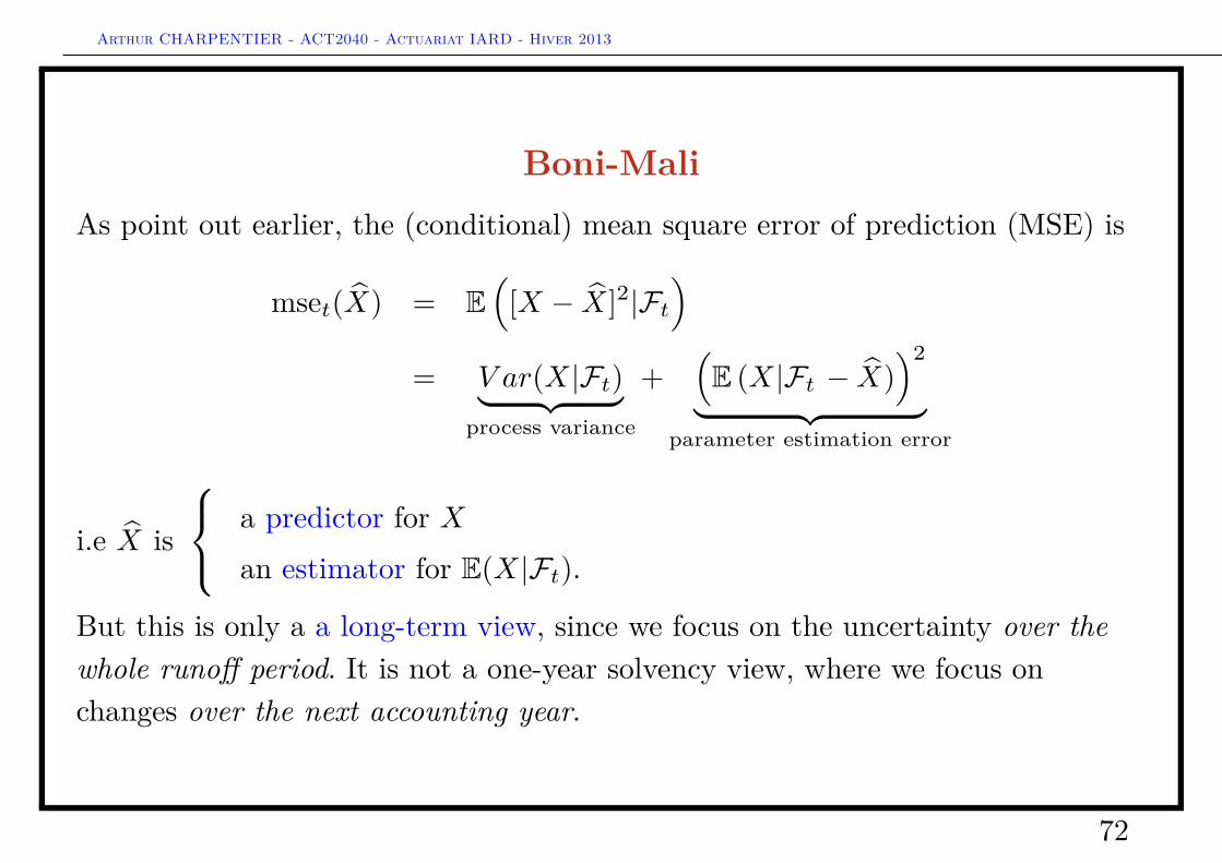
Boni-MaliAs point out earlier, the (conditional) mean square error of prediction (MSE) is
mset(X) = E(
[X − X]2|Ft)
= V ar(X|Ft)︸ ︷︷ ︸process variance
+(E (X|Ft − X)
)2
︸ ︷︷ ︸parameter estimation error
i.e X is
a predictor for Xan estimator for E(X|Ft).
But this is only a a long-term view, since we focus on the uncertainty over thewhole runoff period. It is not a one-year solvency view, where we focus onchanges over the next accounting year.
72

Arthur CHARPENTIER - ACT2040 - Actuariat IARD - Hiver 2013
Boni-Mali
From time t = n and time t = n+ 1,
λj(n)
=∑n−j−1i=0 Ci,j+1∑n−j−1i=0 Ci,j
and λj(n+1)
=∑n−ji=0 Ci,j+1∑n−ji=0 Ci,j
and the ultimate loss predictions are then
C(n)i = Ci,n−i ·
n∏j=n−i
λj(n)
and C(n+1)i = Ci,n−i+1 ·
n∏j=n−i+1
λj(n+1)
73
Arthur CHARPENTIER - ACT2040 - Actuariat IARD - Hiver 2013
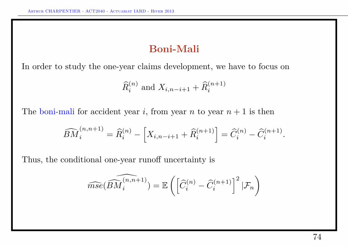
Boni-MaliIn order to study the one-year claims development, we have to focus on
R(n)i and Xi,n−i+1 + R
(n+1)i
The boni-mali for accident year i, from year n to year n+ 1 is then
BM(n,n+1)i = R
(n)i −
[Xi,n−i+1 + R
(n+1)i
]= C
(n)i − C(n+1)
i .
Thus, the conditional one-year runoff uncertainty is
mse(
BM(n,n+1)i ) = E
([C
(n)i − C(n+1)
i
]2|Fn)
74
Arthur CHARPENTIER - ACT2040 - Actuariat IARD - Hiver 2013
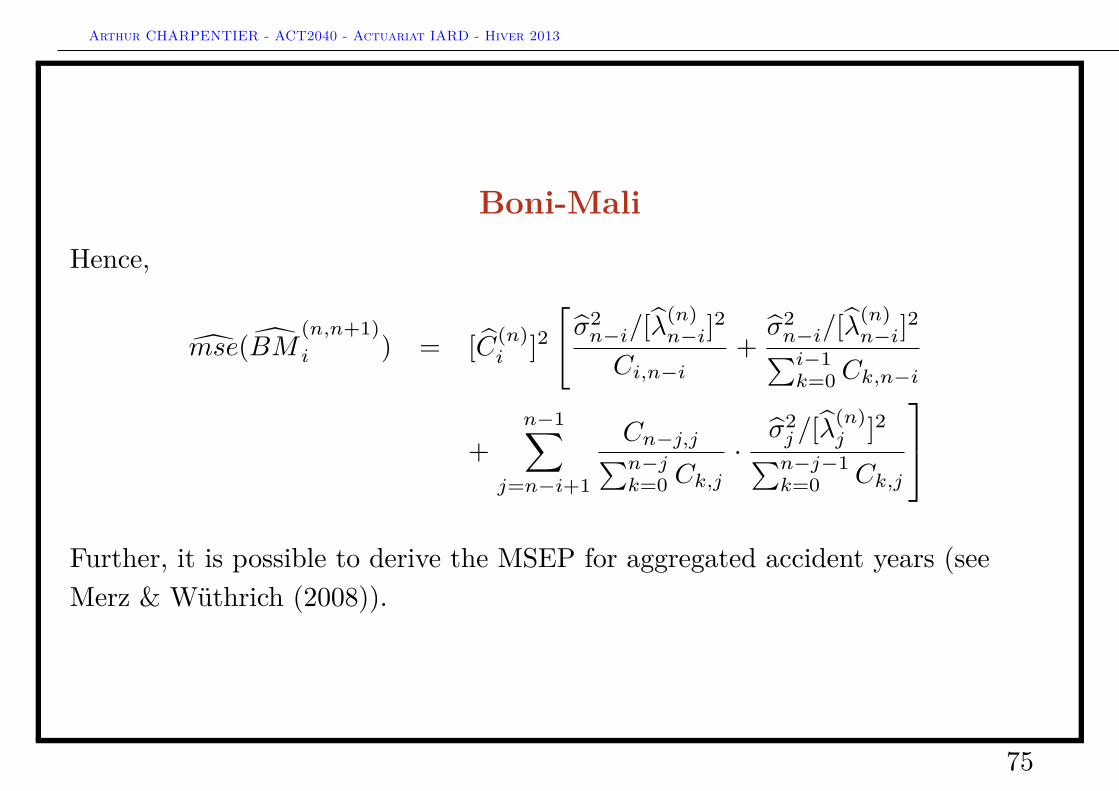
Boni-MaliHence,
mse(BM(n,n+1)i ) = [C(n)
i ]2[σ2n−i/[λ
(n)n−i]2
Ci,n−i+σ2n−i/[λ
(n)n−i]2∑i−1
k=0 Ck,n−i
+n−1∑
j=n−i+1
Cn−j,j∑n−jk=0 Ck,j
·σ2j /[λ
(n)j ]2∑n−j−1
k=0 Ck,j
Further, it is possible to derive the MSEP for aggregated accident years (seeMerz & Wüthrich (2008)).
75
Arthur CHARPENTIER - ACT2040 - Actuariat IARD - Hiver 2013
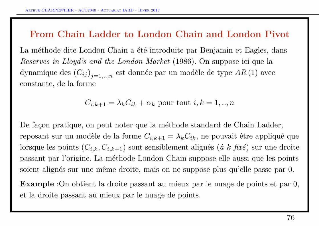
From Chain Ladder to London Chain and London PivotLa méthode dite London Chain a été introduite par Benjamin et Eagles, dansReserves in Lloyd’s and the London Market (1986). On suppose ici que ladynamique des (Cij)j=1,..,n est donnée par un modèle de type AR (1) avecconstante, de la forme
Ci,k+1 = λkCik + αk pour tout i, k = 1, .., n
De façon pratique, on peut noter que la méthode standard de Chain Ladder,reposant sur un modèle de la forme Ci,k+1 = λkCik, ne pouvait être appliqué quelorsque les points (Ci,k, Ci,k+1) sont sensiblement alignés (à k fixé) sur une droitepassant par l’origine. La méthode London Chain suppose elle aussi que les pointssoient alignés sur une même droite, mais on ne suppose plus qu’elle passe par 0.
Example :On obtient la droite passant au mieux par le nuage de points et par 0,et la droite passant au mieux par le nuage de points.
76
Arthur CHARPENTIER - ACT2040 - Actuariat IARD - Hiver 2013
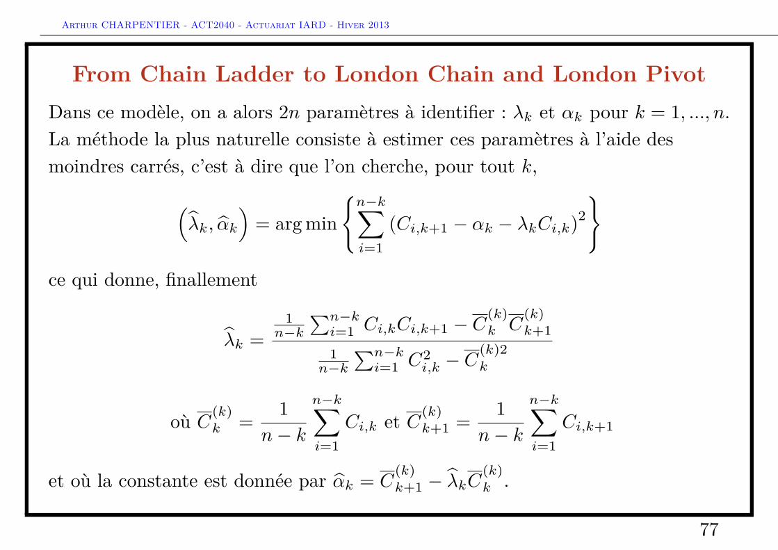
From Chain Ladder to London Chain and London PivotDans ce modèle, on a alors 2n paramètres à identifier : λk et αk pour k = 1, ..., n.La méthode la plus naturelle consiste à estimer ces paramètres à l’aide desmoindres carrés, c’est à dire que l’on cherche, pour tout k,
(λk, αk
)= arg min
{n−k∑i=1
(Ci,k+1 − αk − λkCi,k)2
}ce qui donne, finallement
λk =1
n−k∑n−ki=1 Ci,kCi,k+1 − C
(k)k C
(k)k+1
1n−k
∑n−ki=1 C2
i,k − C(k)2k
où C(k)k = 1
n− k
n−k∑i=1
Ci,k et C(k)k+1 = 1
n− k
n−k∑i=1
Ci,k+1
et où la constante est donnée par αk = C(k)k+1 − λkC
(k)k .
77
Arthur CHARPENTIER - ACT2040 - Actuariat IARD - Hiver 2013
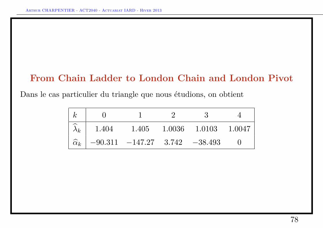
From Chain Ladder to London Chain and London PivotDans le cas particulier du triangle que nous étudions, on obtient
k 0 1 2 3 4
λk 1.404 1.405 1.0036 1.0103 1.0047αk −90.311 −147.27 3.742 −38.493 0
78
Arthur CHARPENTIER - ACT2040 - Actuariat IARD - Hiver 2013
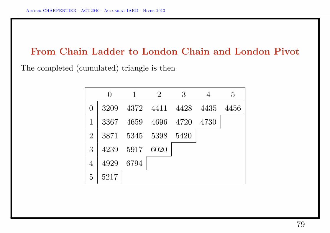
From Chain Ladder to London Chain and London PivotThe completed (cumulated) triangle is then
0 1 2 3 4 50 3209 4372 4411 4428 4435 44561 3367 4659 4696 4720 47302 3871 5345 5398 54203 4239 5917 60204 4929 67945 5217
79

Arthur CHARPENTIER - ACT2040 - Actuariat IARD - Hiver 2013
From Chain Ladder to London Chain and London Pivot0 1 2 3 4 5
0 3209 4372 4411 4428 4435 44561 3367 4659 4696 4720 4730 47522 3871 5345 5398 5420 5437 54633 4239 5917 6020 6045 6069 60984 4929 6794 6922 6950 6983 70165 5217 7234 7380 7410 7447 7483
One the triangle has been completed, we obtain the amount of reserves, withrespectively 22, 43, 78, 222 and 2266 per accident year, i.e. the total is 2631 (tobe compared with 2427, obtained with the Chain Ladder technique).
80
Arthur CHARPENTIER - ACT2040 - Actuariat IARD - Hiver 2013
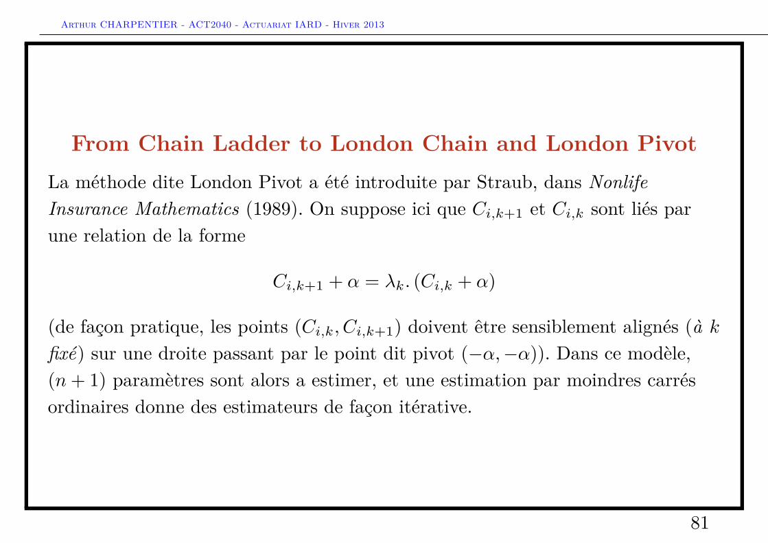
From Chain Ladder to London Chain and London PivotLa méthode dite London Pivot a été introduite par Straub, dans NonlifeInsurance Mathematics (1989). On suppose ici que Ci,k+1 et Ci,k sont liés parune relation de la forme
Ci,k+1 + α = λk. (Ci,k + α)
(de façon pratique, les points (Ci,k, Ci,k+1) doivent être sensiblement alignés (à kfixé) sur une droite passant par le point dit pivot (−α,−α)). Dans ce modèle,(n+ 1) paramètres sont alors a estimer, et une estimation par moindres carrésordinaires donne des estimateurs de façon itérative.
81
Arthur CHARPENTIER - ACT2040 - Actuariat IARD - Hiver 2013
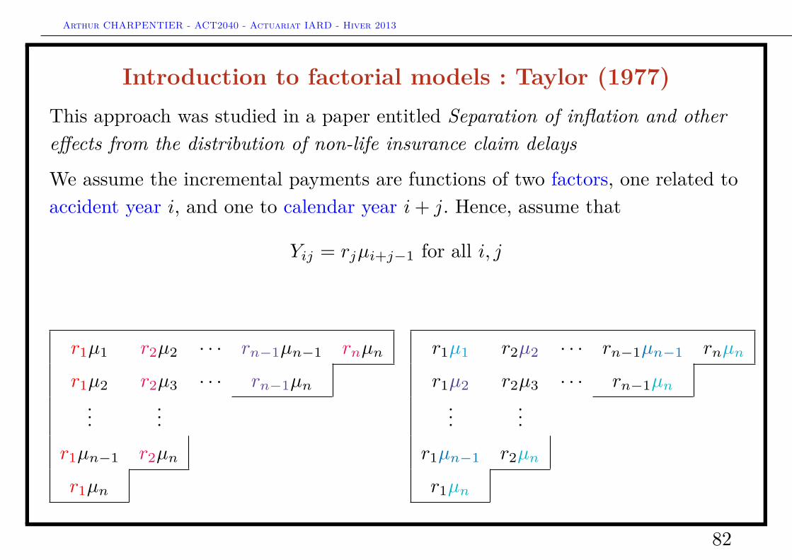
Introduction to factorial models : Taylor (1977)This approach was studied in a paper entitled Separation of inflation and othereffects from the distribution of non-life insurance claim delays
We assume the incremental payments are functions of two factors, one related toaccident year i, and one to calendar year i+ j. Hence, assume that
Yij = rjµi+j−1 for all i, j
r1µ1 r2µ2 · · · rn−1µn−1 rnµn
r1µ2 r2µ3 · · · rn−1µn...
...r1µn−1 r2µn
r1µn
et
r1µ1 r2µ2 · · · rn−1µn−1 rnµn
r1µ2 r2µ3 · · · rn−1µn...
...r1µn−1 r2µn
r1µn
82
Arthur CHARPENTIER - ACT2040 - Actuariat IARD - Hiver 2013
Hence, incremental payments are functions of development factors, rj , and acalendar factor, µi+j−1, that might be related to some inflation index.
83
Arthur CHARPENTIER - ACT2040 - Actuariat IARD - Hiver 2013
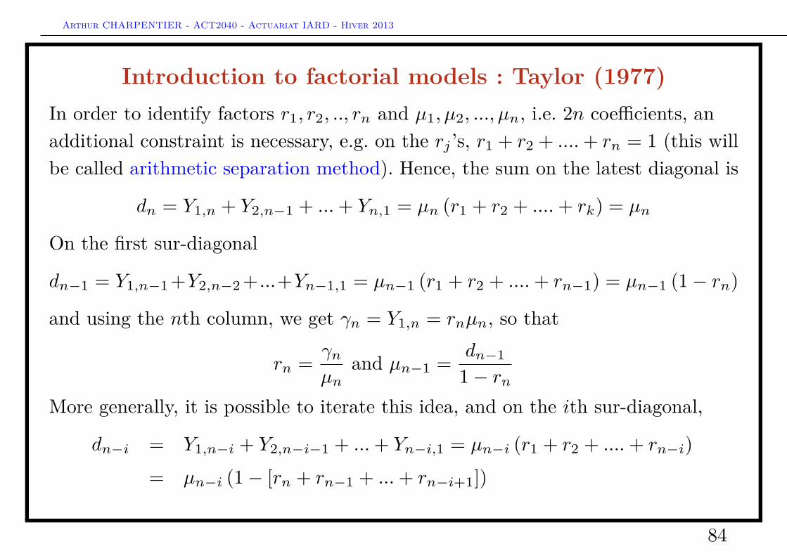
Introduction to factorial models : Taylor (1977)In order to identify factors r1, r2, .., rn and µ1, µ2, ..., µn, i.e. 2n coefficients, anadditional constraint is necessary, e.g. on the rj ’s, r1 + r2 + ....+ rn = 1 (this willbe called arithmetic separation method). Hence, the sum on the latest diagonal is
dn = Y1,n + Y2,n−1 + ...+ Yn,1 = µn (r1 + r2 + ....+ rk) = µn
On the first sur-diagonal
dn−1 = Y1,n−1 +Y2,n−2 + ...+Yn−1,1 = µn−1 (r1 + r2 + ....+ rn−1) = µn−1 (1− rn)
and using the nth column, we get γn = Y1,n = rnµn, so that
rn = γnµn
and µn−1 = dn−1
1− rnMore generally, it is possible to iterate this idea, and on the ith sur-diagonal,
dn−i = Y1,n−i + Y2,n−i−1 + ...+ Yn−i,1 = µn−i (r1 + r2 + ....+ rn−i)= µn−i (1− [rn + rn−1 + ...+ rn−i+1])
84
Arthur CHARPENTIER - ACT2040 - Actuariat IARD - Hiver 2013
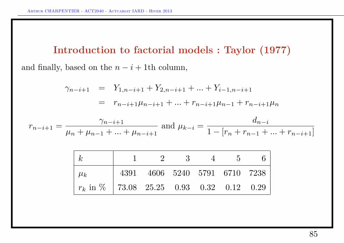
Introduction to factorial models : Taylor (1977)and finally, based on the n− i+ 1th column,
γn−i+1 = Y1,n−i+1 + Y2,n−i+1 + ...+ Yi−1,n−i+1
= rn−i+1µn−i+1 + ...+ rn−i+1µn−1 + rn−i+1µn
rn−i+1 = γn−i+1
µn + µn−1 + ...+ µn−i+1and µk−i = dn−i
1− [rn + rn−1 + ...+ rn−i+1]
k 1 2 3 4 5 6
µk 4391 4606 5240 5791 6710 7238rk in % 73.08 25.25 0.93 0.32 0.12 0.29
85
Arthur CHARPENTIER - ACT2040 - Actuariat IARD - Hiver 2013
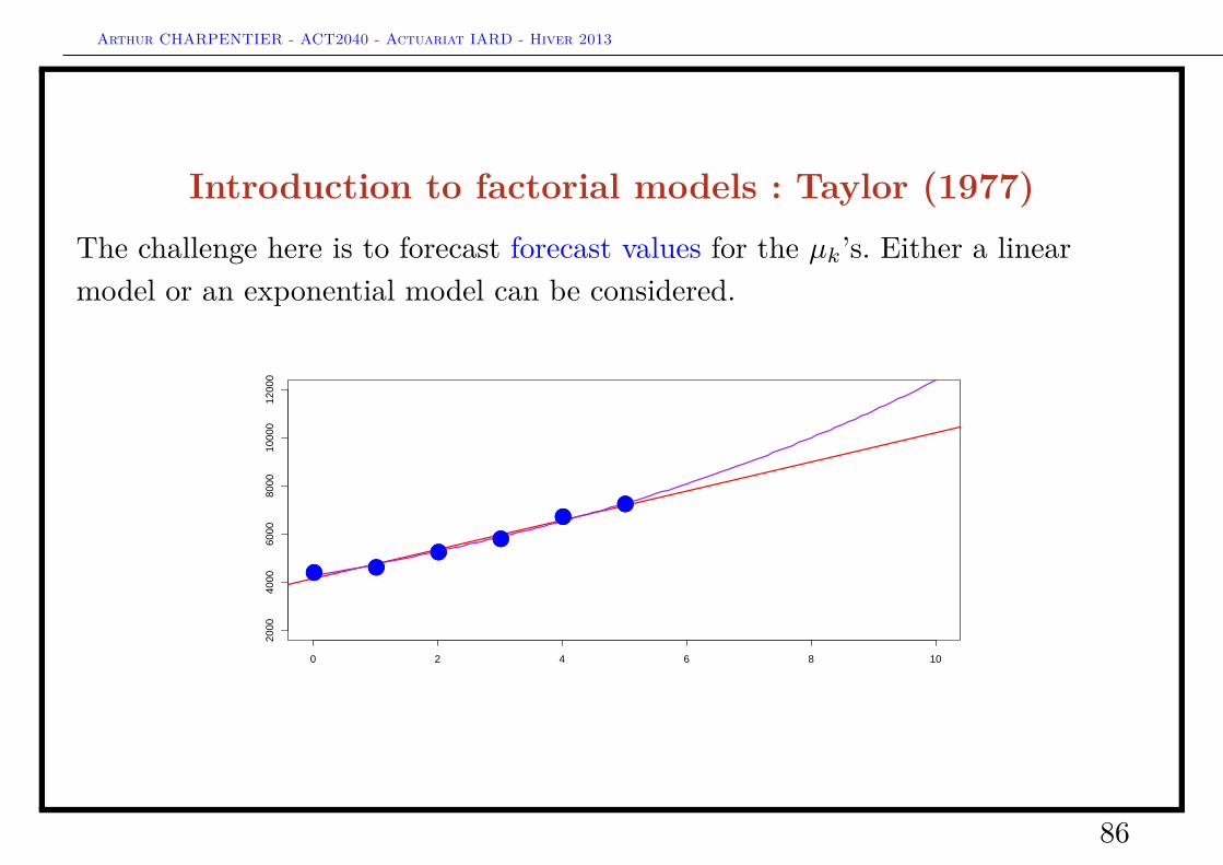
Introduction to factorial models : Taylor (1977)The challenge here is to forecast forecast values for the µk’s. Either a linearmodel or an exponential model can be considered.
● ●●
●●
●
0 2 4 6 8 10
2000
4000
6000
8000
1000
012
000
● ●●
●●
●
86
Arthur CHARPENTIER - ACT2040 - Actuariat IARD - Hiver 2013
Lemaire (1982) and autoregressive modelsInstead of a simple Markov process, it is possible to assume that the Ci,j ’s can bemodeled with an autorgressive model in two directions, rows and columns,
Ci,j = αCi−1,j + βCi,j−1 + γ.
87
Arthur CHARPENTIER - ACT2040 - Actuariat IARD - Hiver 2013
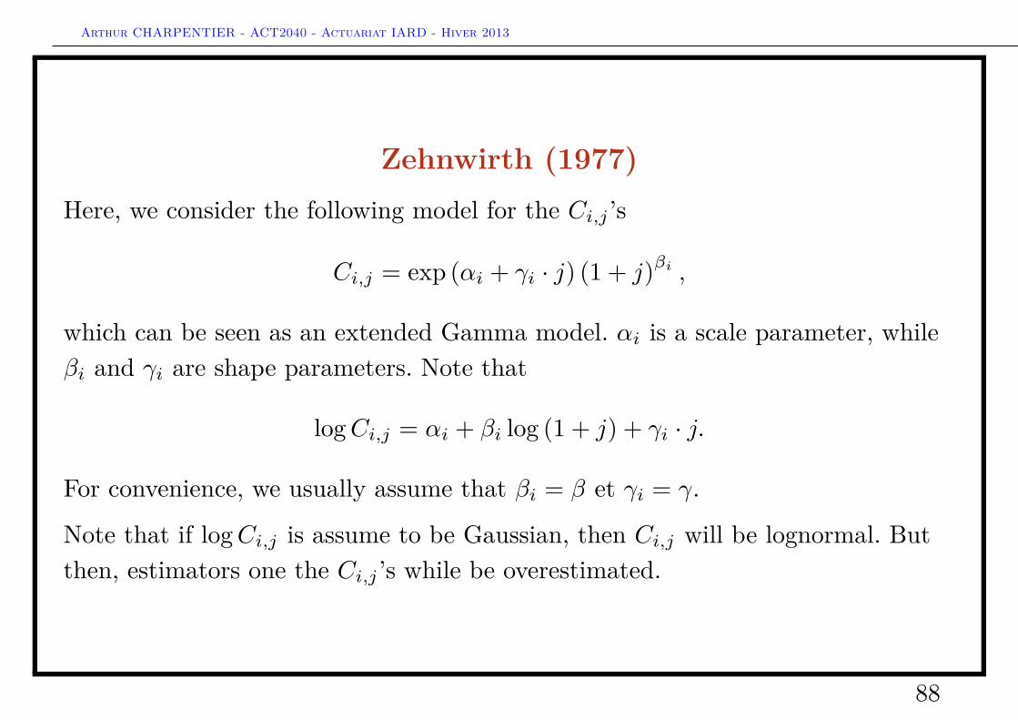
Zehnwirth (1977)Here, we consider the following model for the Ci,j ’s
Ci,j = exp (αi + γi · j) (1 + j)βi ,
which can be seen as an extended Gamma model. αi is a scale parameter, whileβi and γi are shape parameters. Note that
logCi,j = αi + βi log (1 + j) + γi · j.
For convenience, we usually assume that βi = β et γi = γ.
Note that if logCi,j is assume to be Gaussian, then Ci,j will be lognormal. Butthen, estimators one the Ci,j ’s while be overestimated.
88
Arthur CHARPENTIER - ACT2040 - Actuariat IARD - Hiver 2013
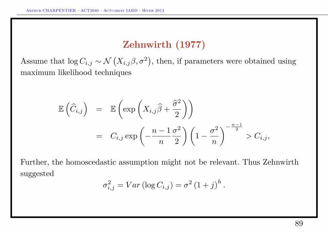
Zehnwirth (1977)Assume that logCi,j ∼ N
(Xi,jβ, σ
2), then, if parameters were obtained usingmaximum likelihood techniques
E(Ci,j
)= E
(exp
(Xi,j β + σ2
2
))
= Ci,j exp(−n− 1
n
σ2
2
)(1− σ2
n
)−n−12
> Ci,j ,
Further, the homoscedastic assumption might not be relevant. Thus Zehnwirthsuggested
σ2i,j = V ar (logCi,j) = σ2 (1 + j)h .
89
Arthur CHARPENTIER - ACT2040 - Actuariat IARD - Hiver 2013
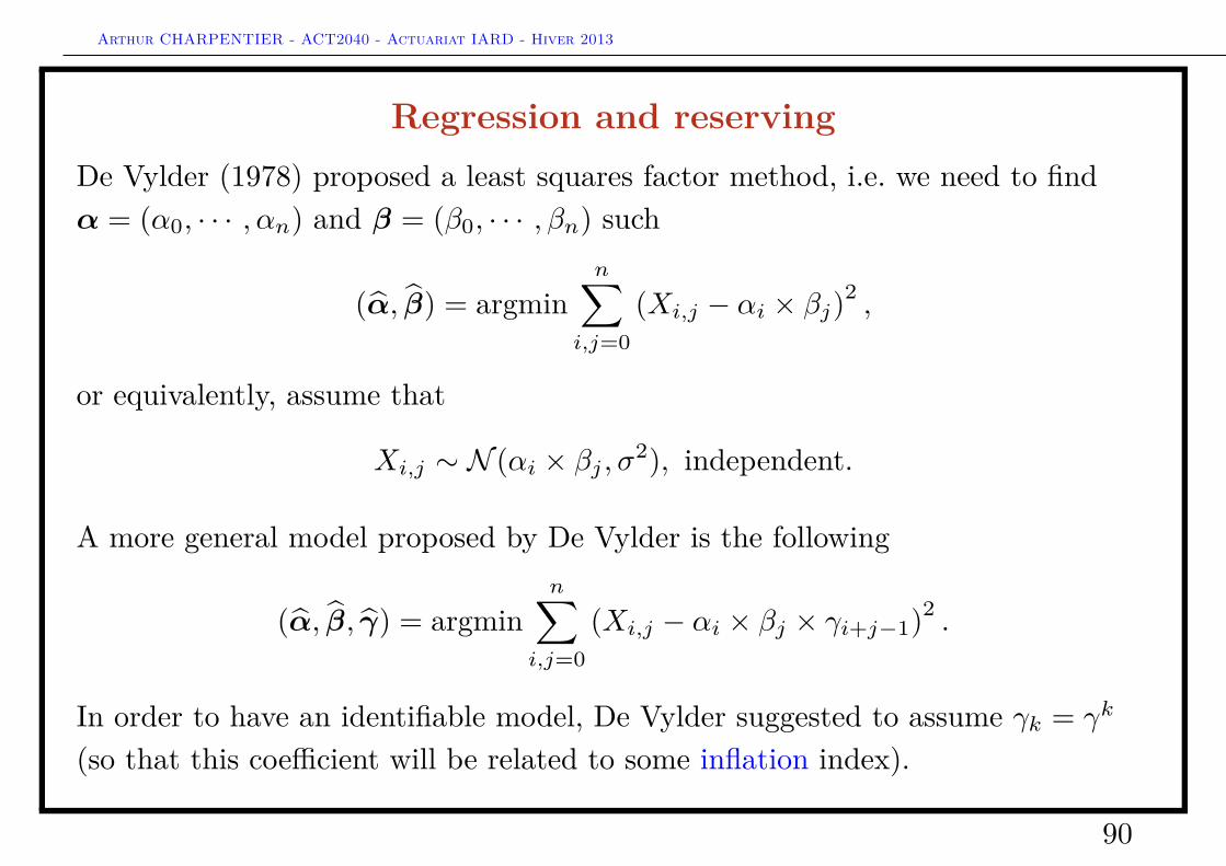
Regression and reservingDe Vylder (1978) proposed a least squares factor method, i.e. we need to findα = (α0, · · · , αn) and β = (β0, · · · , βn) such
(α, β) = argminn∑
i,j=0(Xi,j − αi × βj)2
,
or equivalently, assume that
Xi,j ∼ N (αi × βj , σ2), independent.
A more general model proposed by De Vylder is the following
(α, β, γ) = argminn∑
i,j=0(Xi,j − αi × βj × γi+j−1)2
.
In order to have an identifiable model, De Vylder suggested to assume γk = γk
(so that this coefficient will be related to some inflation index).
90