Actualisatie en verfijning voor Vlaanderen · Koning Albert-II laan 20 1000 Brussel ... 6...

Actualisatie en verfijning klimaatscenario’s tot 2100 voor Vlaanderen

Appendix 2: Nieuwe modelprojecties voor Ukkel op basis van globale klimaatmodellen (CMIP5) en actualisatie klimaatscenario’s

Studie uitgevoerd in opdracht van MIRA, Milieurapport Vlaanderen

Onderzoeksrapport MIRA/2015/03, januari 2015

Actualisatie en verfijning klimaatscenario’s tot 2100 voor Vlaanderen

Appendix 2: Nieuwe modelprojecties voor Ukkel op basis van globale klimaatmodellen (CMIP5)

en actualisatie klimaatscenario’s

Hossein Tabari, Meron Teferi Taye, Patrick Willems

Afdeling Hydraulica KU Leuven

Studie uitgevoerd in opdracht van MIRA, Milieurapport Vlaanderen

MIRA/2015/03

Januari 2015

2

Documentbeschrijving Titel Actualisatie en verfijning klimaatscenario’s tot 2100 voor Vlaanderen - Appendix 2: Nieuwe modelprojecties voor Ukkel op basis van globale klimaatmodellen (CMIP5) en actualisatie klimaatscenario’s

Dit rapport verschijnt in de reeks MIRA Ondersteunend Onderzoek van de Vlaamse Milieumaatschappij. Deze reeks bevat resultaten van onderzoek gericht op de wetenschappelijke onderbouwing van het Milieurapport Vlaanderen.

Het rapport geldt tevens als eindrapport van de studie ‘Bijsturing klimaatscenario’s voor hydrologische & hydrodynamische impactanalyse - Statistische analyse nieuwe CMIP5 klimaatmodelruns voor België’ voor de Afdeling Operationeel Waterbeheer van de Vlaamse Milieumaatschappij. Samenstellers Hossein Tabari, Meron Teferi Taye, Patrick Willems Afdeling Hydraulica, KU Leuven Samenwerking De hoge-resolutie klimaatmodelresultaten voor België (ALARO-model en MACCBET-project; zie Deel 5 in dit rapport) werden ter beschikking gesteld door: Rozemien De Troch, Piet Termonia, Koninklijk Meteorologisch Instituut van België Sajjad Saeed, Nicole van Lipzig, Afdeling Aard- en Omgevingswetenschappen en Afdeling Hydraulica, KU Leuven Wetenschappelijke begeleidingsgroep

Dit rapport kwam tot stand in samenwerking met de volgende wetenschappelijke begeleidingsgroep:

Johan Brouwers (MIRA VMM)

Bob Peeters (MIRA VMM)

Johan Bogaert (Dept. LNE)

Michel Craninx, Kris Cauwenberghs (Afdeling Operationeel Waterbeheer VMM)

Juliette Dujardin, Sandy Adriaenssens (IRCEL & VMM)

Fernando Pereira (MOW, Waterbouwkundig Laboratorium)

Koen De Ridder (VITO)

Martine Vanderstraeten (BELSPO)

Dominique Fonteyn (BIRA, Federaal instituut voor klimaatdiensten)

Jean-Pascal van Ypersele (UCL/IPCC)

Inhoud Dit is de 2

e technische Appendix (Engelstalig) bij het MIRA rapport ‘Actualisatie en verfijning

klimaatscenario’s tot 2100 voor Vlaanderen’ en tevens het eindrapport bij de parallele studie voor de Afdeling Operationeel Waterbeheer van de VMM. Ze rapporteert de resultaten van de CMIP5-modellen, die werden geanalyseerd voor Ukkel, aangevuld met bijkomende analyses om inzicht te geven in de exacte positie van de hoge-resolutie Belgische klimaatmodelresultaten (zie Appendix 1) binnen de bandbreedte die het IPCC naar voren schuift. Deze analyse was noodzakelijk om de hoge-resolutie klimaatruns te kunnen interpreteren. Vanwege de hoge computerkosten die de hoge-resolutie runs met zich meebrengen, werden voor België slechts twee CMIP5 modellen (EC-Earth-KU Leuven en Arpege-KMI) dynamisch neergeschaald (zie Appendix 1 bij dit MIRA-rapport). Een presentatie van enkel deze runs kan een vertekend beeld geven naar beleidsmakers toe en daarom is het kaderen in de bandbreedte van het IPCC absoluut noodzakelijk. Dit gebeurt in dit rapport. Daarna beschrijft dit rapport de nieuwe klimaatscenario’s, afgeleid op basis van die uitgebreide set aan nieuwe CMIP5-klimaatmodelsimulaties. In het kader van de parallelle studie voor de Afdeling Operationeel Waterbeheer van de VMM werden deze resultaten verder verwerkt tot het afleiden van klimaatscenario’s die specifiek bruikbaar zijn voor hydrologische en hydraulische impactanalyses, na toepassing van statistische neerschaling en de methode beschreven in Ntegeka et al. (2014).

3

Wijze van refereren Tabari H., Taye M.T. & Willems P. (2015), Actualisatie en verfijning klimaatscenario’s tot 2100 voor Vlaanderen - Appendix 2: Nieuwe modelprojecties voor Ukkel op basis van globale klimaatmodellen (CMIP5). Studie uitgevoerd in opdracht van de Afdeling Operationeel Waterbeheer van de Vlaamse Milieumaatschappij en MIRA, MIRA/2015/03, KU Leuven. Raadpleegbaar op www.milieurapport.be. Vragen in verband met dit rapport Vlaamse Milieumaatschappij Milieurapportering (MIRA) Van Benedenlaan 34 2800 Mechelen tel. 015 45 14 61 [email protected] Afdeling Operationeel Waterbeheer Dienst hoogwater Graaf de Ferraris-gebouw Koning Albert-II laan 20 1000 Brussel tel. 02 553 21 06 [email protected] D/2015/6871/006 ISBN 9789491385414 NUR 973/943

http://www.milieurapport.be/

mailto:[email protected]

mailto:[email protected]

4

Contents

Inleiding en samenvatting ..................................................................................................... 12

0 Introduction ............................................................................................................... 16

1 New RCP based greenhouse concentration scenarios - introduction ................ 16 1.1 SRES scenarios ............................................................................................. 16 1.2 RCP based scenarios ..................................................................................... 17 1.3 Practical use of the climate scenarios for decision making ............................ 19

2 Overview of GCM and RCM runs ............................................................................. 21

3 Statistical analysis of CMIP5 GCM runs ................................................................. 27 3.1 ETo calculation ............................................................................................... 27 3.2 Validation of control runs ................................................................................ 30

3.2.1 Precipitation ........................................................................................ 30 3.2.2 Temperature ....................................................................................... 32 3.2.3 ETo ..................................................................................................... 33 3.2.4 Conclusions ........................................................................................ 34

3.3 Climate changes: scenario vs. control runs ................................................... 35 3.3.1 Precipitation ........................................................................................ 35 3.3.2 Temperature ....................................................................................... 39 3.3.3 ETo ..................................................................................................... 42 3.3.4 Correlation precipitation-T/ETo changes ............................................ 43 3.3.5 Conclusions ........................................................................................ 47

4 Statistical analysis of CORDEX RCM runs and differences with CMIP5 GCM runs and CCI-HYDR scenarios ............................................................................................. 48

4.1 Precipitation .................................................................................................... 48 4.1.1 Changes in number of wet days ......................................................... 48 4.1.2 Changes in mean monthly/seasonal values ....................................... 49 4.1.3 Changes in wet day quantiles ............................................................ 50

4.2 Temperature ................................................................................................... 53 4.3 ETo ................................................................................................................. 56 4.4 Seasonal water balance ................................................................................. 61 4.5 Wind speed ..................................................................................................... 62 4.6 Correlation between precipitation and temperature changes ........................ 63 4.7 Conclusions .................................................................................................... 65

5 Statistical analysis of high resolution climate model runs for Belgium ............. 66 5.1 Overview high resolution model runs for Belgium .......................................... 66 5.2 Validation and analysis of ALARO high resolution model results .................. 68 5.3 Validation and analysis of MACCBET high resolution model results ............. 75 5.4 Spatial differences .......................................................................................... 78 5.5 Conclusions .................................................................................................... 81

6 Statistical downscaling and update perturbation tool .......................................... 82 6.1 Review on statistical downscaling methods ................................................... 82 6.2 Testing assumptions selected statistical downscaling method ...................... 84 6.3 Perturbation tool ............................................................................................. 86

References .............................................................................................................................. 88

Annex A: Individual climate model results .......................................................................... 90 Number of wet days changes ...................................................................................... 90 Mean seasonal precipitation changes ......................................................................... 91

5

Monthly change factors of ‘best’ models ..................................................................... 92 Wet day precipitation quantiles changes ..................................................................... 92

Annex B: Climate model results versus observations ....................................................... 96 Daily precipitation quantiles: per month ...................................................................... 96 Monthly mean temperature ....................................................................................... 100 Daily temperature quantiles: per season ................................................................... 101 Daily temperature quantiles: per month .................................................................... 102

6

Figures Figure 0.1: Total carbon dioxide emissions for the SRES scenarios (4 ‘marker’ scenarios and A1

Fossil Intensive scenario (coloured lines) (IPCC, 2007). Illustrative carbon dioxide emissions for each

of the representative concentration pathways (grey lines) ................................................................... 17 Figure 0.2: Approaches to the development of climate forcing scenarios: (a) previous sequential

approach for the SRES emission scenarios; (b) parallel approach of the RCP based scenarios ........ 18 Figure 0.3: Simplified chart of the main processes involved in modelling hydrological impacts from

climate change ...................................................................................................................................... 19 Figure 0.4: Historical versus projected changes in global CO2 emissions............................................ 20 Figure 3.1: Mean monthly precipitation for the different CMIP5 GCM control runs (1961-1990) ......... 30 Figure 3.2: Wet day precipitation intensities vs. return period: validation of CMIP5 GCM runs based on

Uccle historical observations (1961-1990), for winter season .............................................................. 31 Figure 3.3: Wet day precipitation intensities vs. return period: validation of CMIP5 GCM runs based on

Uccle historical observations (1961-1990), for summer season ........................................................... 31 Figure 3.4: Mean monthly temperature for the different CMIP5 GCM control runs (1961-1990) ......... 32 Figure 3.5: Temperature vs. return period: validation of CMIP5 GCM runs based on Uccle historical

observations (1961-1990), for winter and summer season .................................................................. 32 Figure 3.6: Mean monthly ETo for the different CMIP5 GCM control runs (1961-1990) ...................... 33 Figure 3.7: Evapotranspiration vs. return period: validation of CMIP5 GCM runs based on Uccle

historical observations (1961-1990), for winter and summer season ................................................... 34 Figure 3.8: Change factors in the number of wet days for all RCP scenarios highlighting high, mean

and low scenarios ................................................................................................................................. 36 Figure 3.9: Mean monthly precipitation for the different CMIP5 GCM future runs (2071-2100), for

combined RCP scenarios, median of control runs (1961-1990) and Uccle observation ...................... 36 Figure 3.10: Mean monthly precipitation for the different CMIP5 GCM future runs (2071-2100), for the

individual RCP scenarios, median of control runs (1961-1990) and Uccle observation ....................... 37 Figure 3.11: Wet day precipitation intensities vs. return period: comparison of CMIP5 GCM control

(1961-1990) with Uccle observation and scenario (2071-2100) runs with median of control runs, for all

RCP scenarios and winter season ........................................................................................................ 38 Figure 3.12: Wet day precipitation intensities vs. return period: comparison of control (1961-1990) with

Uccle observation and scenario (2071-2100) runs with median of control runs, for all RCP scenarios

and summer season .............................................................................................................................. 38 Figure 3.13: Wet day relative change calculated based on control (1961-1990) and scenario (2071-

2100) runs versus return periods, for all RCP scenarios and winter season (left) and summer season

(right) ..................................................................................................................................................... 39 Figure 3.14: Mean monthly temperature for the different CMIP5 GCM future runs (2071-2100), for

combined RCP scenarios, median of control runs (1961-1990) and Uccle observation ...................... 39 Figure 3.15: Mean monthly temperature for the different CMIP5 GCM future runs (2071-2100), for the

individual RCP scenarios, median of control runs (1961-1990) and Uccle observation ....................... 40 Figure 3.16: Mean monthly temperature changes for the different CMIP5 GCM runs using all RCP

scenarios ............................................................................................................................................... 40 Figure 3.17: Temperature vs. return period: comparison of CMIP5 GCM control (1961-1990) and

scenario (2071-2100) runs, for all RCP scenarios and winter season ................................................. 41 Figure 3.18: Temperature vs. return period: comparison of control (1961-1990) and scenario (2071-

2100) runs, for all RCP scenarios and summer season ....................................................................... 41 Figure 3.19: Temperature change vs. return period for all RCP scenarios, winter and summer season

.............................................................................................................................................................. 42 Figure 3.20: Mean monthly ETo for the different CMIP5 GCM future runs (2071-2100), for combined

RCP scenarios, median of control runs (1961-1990) and Uccle observation ....................................... 42 Figure 3.21: ETo change factors vs. return period for the different CMIP5 GCM runs, all RCP

scenarios combined, for winter and summer seasons .......................................................................... 43

7

Figure 3.22: Inter-seasonal tracing of precipitation and temperature relative changes (averaged for

return periods >0.1 year) for the different RCP scenarios .................................................................... 44 Figure 3.23: Inter-seasonal tracing of precipitation and temperature relative changes (averaged for

return periods >1 year) for the different RCP scenarios ....................................................................... 45 Figure 3.24: Inter-seasonal tracing of precipitation and temperature relative changes (averaged for

return periods >5 years) for the different RCP scenarios ..................................................................... 45 Figure 3.25: Inter-seasonal tracing of precipitation and ETo relative changes (averaged for return

periods >0.1 year) for the different RCP scenarios ............................................................................... 46 Figure 4.1: High, mean and low scenarios extracted from CMIP5 GCM runs for change in number of

wet days (left) and dry days (right) over 100 years ............................................................................... 49 Figure 4.2: High, mean and low scenarios extracted from CMIP5 GCM runs and CORDEX RCM runs

(left) and high, mean and low scenarios extracted from CMIP5 GCM runs and the PRUDENCE and

ENSEMBLES RCM runs (right) over 100 years.................................................................................... 49 Figure 4.3: High, mean and low scenarios extracted from CMIP5 GCM runs and the PRUDENCE and

ENSEMBLES RCM runs over 30 years (left) and 50 years (right) ....................................................... 50 Figure 4.4: High, mean and low relative change values of wet day precipitation intensities vs. return

period: comparison between the CMIP5 GCM runs and CORDEX RCM runs, for winter and summer

seasons over 100 years ........................................................................................................................ 51 Figure 4.5: Comparison of precipitation relative changes computed using the full range of CMIP5

GCM runs and CORDEX runs for winter and summer season ............................................................. 52 Figure 4.6: Comparison of precipitation relative changes computed using RCP4.5 scenarios of CMIP5

GCM runs and CORDEX runs for winter and summer season ............................................................. 52 Figure 4.7: Comparison of precipitation relative changes computed using RCP4.5 scenarios of CMIP5

GCM runs and CORDEX runs for winter and summer season ............................................................. 52 Figure 4.8: High, mean and low scenarios extracted from CMIP5 GCM runs and the CORDEX RCM

runs for temperature changes (left) and high, mean and low scenarios extracted from CMIP5 GCM

runs and the CCI-HYDR RCM runs (right) over 100 years ................................................................... 54 Figure 4.9: High, mean and low scenarios extracted from CMIP5 GCM runs and the CORDEX RCM

runs for temperature changes (top) and high, mean and low scenarios extracted from CMIP5 GCM

runs and the CCI-HYDR RCM runs (bottom) over 30 years (left) and 50 years (right) ........................ 54 Figure 4.10: High, mean and low relative change values of daily temperature vs. return period:

comparison between the CMIP5 GCM runs and CORDEX RCM runs, for winter and summer seasons

over 100 years ...................................................................................................................................... 55 Figure 4.11: Comparison of temperature changes computed using RCP4.5 scenarios of CMIP5 GCM

runs and CORDEX runs for winter and summer season ...................................................................... 56 Figure 4.12: High, mean and low scenarios extracted from CMIP5 GCM runs and the CCI-HYDR

RCM runs for ETo change factors over 100 years................................................................................ 56 Figure 4.13: High, mean and low scenarios extracted from CMIP5 GCM runs and the CCI-HYDR

RCM runs for ETo change factors over 30 years (left) and 50 years (right) ......................................... 57 Figure 4.14: Sensitivity analysis of ETo change due to individual variables ........................................ 58 Figure 4.15: ETo estimates of the Bultot and Penman–Monteith FAO 56 (PMF-56) methods for

historical period (1961-1990) for GFDL-CM3 model run ...................................................................... 59 Figure 4.16: ETo vs. return period: comparison of the Bultot and Penman–Monteith FAO 56 (PMF-56)

methods for historical period (1961-1990), for winter and summer season ......................................... 60 Figure 4.17: Net rainfall for current period (1961-1990) and future period (2071-2100) of CMIP5

GCMs, for scenarios that lead to high positive changes in winter and high negative changes in

summer, considering correlations of precipitation and ETo change scenarios .................................... 61 Figure 4.18: Net rainfall deficit throughout a year at the end of the century using high correlation of

precipitation and ETo change scenarios of CMIP5 GCMs ................................................................... 62 Figure 4.19: High, mean and low scenarios extracted from CMIP5 GCM runs for wind speed change

over 100 years ...................................................................................................................................... 62

8

Figure 4.20: High, mean and low scenarios extracted from CMIP5 GCM runs for wind speed change

over 30 years (left) and 50 years (right) ................................................................................................ 63 Figure 4.21: Inter-seasonal tracing of precipitation and temperature relative changes (averaged for

return periods >0.1 year, over 100 years) for CORDEX and GCM scenarios ...................................... 64 Figure 4.22: Inter-seasonal tracing of precipitation and temperature relative changes (averaged for

return periods >1 year, over 100 years) for CORDEX and GCM scenarios ......................................... 65 Figure 5.1: Comparison of the CNRM–CM3/ALARO results with the CMIP5 ensemble and Uccle

observations, for monthly mean precipitation (historical climate: 1961-1990) ...................................... 69 Figure 5.2: Comparison of the CNRM–CM3/ALARO results with the CMIP5 ensemble and Uccle

observations, for monthly mean precipitation (future climate: 2071-2100) ........................................... 70 Figure 5.3: Comparison of the CNRM–CM3/ALARO 4 km results with the CMIP5 ensemble and Uccle

observations, for daily precipitation quantiles (historical climate: 1961-1990, JJA) .............................. 70 Figure 5.4: Comparison of the ERA40/ALARO 4km results with the CMIP5 ensemble and Uccle

observations, for daily precipitation quantiles (historical climate: 1961-1990, JJA) .............................. 71 Figure 5.5: Comparison of the ERA40/ALARO 4, 10, 40 km and ERA40/ALADIN 25 km results with

ERA40 and Uccle observations, for daily precipitation quantiles (historical climate: 1961-1990, JJA) 71 Figure 5.6: Comparison of the CNRM–CM3/ALARO 4 km results with the CMIP3 and CMIP5 CNRM

runs, PRUDENCE and ENSEMBLES RCMs and Uccle observations, for daily precipitation quantiles

(historical climate: 1961-1990, JJA) ...................................................................................................... 72 Figure 5.7: Comparison of CNRM–CM3/ALARO change factors for 2071-2100 vs. 1961-1990 with

those of the CMIP5 ensemble for the winter season (DJF) .................................................................. 72 Figure 5.8: Comparison of CNRM–CM3/ALARO change factors for 2071-2100 vs. 1961-1990 with

those of the CMIP5 ensemble for the summer season (JJA) ............................................................... 73 Figure 5.9: Comparison of change factor computed using the CNRM–CM3/ALARO 4 km, the CMIP3

and CMIP5 CNRM runs, PRUDENCE and ENSEMBLES RCMs for winter season (DJF) .................. 73 Figure 5.10: Comparison of change factor computed using the CNRM–CM3/ALARO 4 km, the CMIP3

and CMIP5 CNRM runs, PRUDENCE and ENSEMBLES RCMs for summer season (JJA) ............... 74 Figure 5.11: Comparison of hourly maximum precipitation using ERA40/ALARO 4, 10, 40 km and

Uccle observations (historical climate: 1961-1990, JJA) ...................................................................... 74 Figure 5.12: Comparison of the MACCBET results with Uccle observations, for monthly mean

precipitation (historical climate: 2001-2010) ......................................................................................... 75 Figure 5.13: Comparison of the MACCBET results with Uccle observations, for daily extreme

precipitation of winter and summer seasons (historical climate: 2001-2010) ....................................... 75 Figure 5.14: Comparison of the MACCBET future scenarios (2060-2069) with its control run and Uccle

observations (1961-1990), for daily extreme precipitation of winter and summer seasons ................. 76 Figure 5.15: Comparison of change factor computed using the MACCBET (for 2060-2069 horizon)

and CMIP5 (for 2071-2100 horizon) runs for winter and summer seasons .......................................... 76 Figure 5.16: Comparison of the MACCBET results with Uccle observations, for hourly extreme

precipitation of winter and summer seasons (historical climate: 2001-2010) ....................................... 77 Figure 5.17: Comparison of change factor computed using the MACCBET daily and hourly runs for

2060-2069 horizon and for winter and summer seasons ...................................................................... 77 Figure 5.18: 30-year (2071-2100) seasonal mean precipitation anomaly relative to the 30-year mean

of the period 1961-1990 ........................................................................................................................ 78 Figure 5.19: Regional differences across Belgium of the mean seasonal rainfall change over

100 years for the winter (left figure) and summer (right figure), based on the available ensemble of

high-resolution climate runs .................................................................................................................. 79 Figure 5.20: Regional differences across Belgium of the mean annual temperature change over

100 years, based on the available ensemble of high-resolution climate runs ...................................... 79 Figure 5.21: Regional differences across Belgium of the changes of number of days with daily

temperature above 25 °C (left figure) or below 0 °C (right figure), based on the available ensemble of

high-resolution climate runs .................................................................................................................. 80 Figure 6.1: General methodology of precipitation perturbation ............................................................. 83

9

Figure 6.2: Illustration of absolute and relative change factor calculation ............................................ 83 Figure 6.3: Impact of eight downscaling methods on peak flow projection of Grote Nete using rainfall-

runoff models (VHM, NAM and HBV), for summer period .................................................................... 84 Figure 6.4: Comparison of hourly (left) and daily (right) precipitation extremes in the summer season

for the different resolution and generation climate models ................................................................... 85 Figure 6.5: Comparison of change factor computed for the different resolution and generation climate

models ................................................................................................................................................... 85 Figure A.1: Mean seasonal number of wet days change summarized for all the seasons based on

CMIP5 runs ........................................................................................................................................... 90 Figure A.2: Mean seasonal number of wet days change summarized for all the seasons based on

PRUDENCE and ENSMBLES runs ...................................................................................................... 90 Figure A.3: Mean seasonal precipitation change summarized for all the seasons based on CMIP5

runs ....................................................................................................................................................... 91 Figure A.4: Mean seasonal precipitation change summarized for all the seasons based on

PRUDENCE and ENSMBLES runs ...................................................................................................... 91 Figure A.5: High, mean and low scenarios extracted from the ‘best’ CMIP5 GCM runs ...................... 92 Figure A.6: Wet day change factors calculated based on control (1961-1990) and scenario (2071-

2100) runs versus return periods, for RCP2.6 scenarios and one representative month from each

season ................................................................................................................................................... 92 Figure A.7: Wet day change factors calculated based on control (1961-1990) and scenario (2071-







2100) runs versus return periods, for PRUDENCE runs and one representative month from each


2100) runs versus return periods, for ENSEMBLES runs and one representative month from each

season ................................................................................................................................................... 95 Figure B.1: Wet day precipitation intensities vs. return period: validation of CMIP5 GCM runs based

on Uccle historical observations (1961-1990) (left) and comparison with CMIP5 GCM scenario runs

(2071-2100) (right), for January to March ............................................................................................. 96 Figure B.2: Wet day precipitation intensities vs. return period: validation of CMIP5 GCM runs based


(2071-2100) (right), for April to June ..................................................................................................... 97 Figure B.3: Wet day precipitation intensities vs. return period: validation of CMIP5 GCM runs based


(2071-2100) (right), for July to September ............................................................................................ 98 Figure B.4: Wet day precipitation intensities vs. return period: validation of CMIP5 GCM runs based


(2071-2100) (right), for October to December ...................................................................................... 99 Figure B.5: Mean monthly temperature for all CMIP5 GCM runs for the control and future period ... 100 Figure B.6: Mean monthly temperature for all CMIP5 GCM future runs for individual RCP scenarios

............................................................................................................................................................ 100 Figure B.7: Temperature vs. return period: comparison of control and scenario period runs for winter

(top) and summer (bottom) seasons ................................................................................................... 101

10

Figure B.8: Temperature vs. return period: comparison of control and scenario period runs for months

January to March ................................................................................................................................ 102 Figure B.9: Temperature vs. return period: comparison of control and scenario period runs for months

April to June ........................................................................................................................................ 103 Figure B.10: Temperature vs. return period: comparison of control and scenario period runs for

months July to September .................................................................................................................. 104 Figure B.11: Temperature vs. return period: comparison of control and scenario period runs for

months October to December ............................................................................................................. 105

11

Tables Table 0.1: SRES scenario summary ..................................................................................................... 16 Table 0.2: RCP radiative forcing information ........................................................................................ 18 Table 2.1: Downloaded CMIP5 GCM runs (>200 in total) .................................................................... 21 Table 2.2: CORDEX runs considered in this project ............................................................................. 22 Table 2.3: CMIP3 GCM runs considered for the CCI-HYDR based scenarios ..................................... 23 Table 2.4: Matrix of RCM-GCM combinations considered in PRUDENCE RCM runs and sources of

RCMs .................................................................................................................................................... 24 Table 2.5: Matrix of RCM-GCM combinations considered in ENSEMBLES RCM runs and sources of

RCMs .................................................................................................................................................... 24 Table 2.6: Number of runs used in for precipitation analysis (136 runs) .............................................. 25 Table 2.7: Number of runs used in for temperature analysis (71 runs) ................................................ 26 Table 2.8: Number of runs used in for potential evapotranspiration analysis (33 runs) ....................... 26 Table 3.1: Monthly values of the free water surface albedo under clear sky as a function of relative

insolation at 50o latitude ........................................................................................................................ 28

Table 3.2: Seasonal radiation parameters for the Bultot method ......................................................... 28 Table 3.3: Min-max perturbation of mean seasonal precipitation for the CMIP5 GCM runs, different

RCP scenarios, and seasons ................................................................................................................ 37 Table 4.1: Projected change (%) in number of wet days in winter and summer seasons over 100 years

.............................................................................................................................................................. 48 Table 4.2: Projected change (%) in mean seasonal values in winter and summer seasons over

100 years............................................................................................................................................... 50 Table 4.3: High-mean-low change factors of wet day precipitation intensities over 100 years ............ 51 Table 4.4: Projected change (°C) in mean annual temperature over 100 years .................................. 53 Table 4.5: Annual changes in number of days (in comparison with the number of days in the control

period) with mean daily temperature higher than 25 °C and lower than 0 °C....................................... 53 Table 4.6: Projected temperature change (°C) in mean seasonal values in winter and summer

seasons over 100 years ........................................................................................................................ 55 Table 4.7: Projected evapotranspiration change (%) in mean seasonal values in winter and summer

seasons over 100 years ........................................................................................................................ 57 Table 4.8: Percent changes in daily ETo (return period >0.1 years) due to change in each

meteorological variable based on GFDL-CM3 model’s data under RCP8.5 scenario.......................... 57 Table 4.9: Estimated sensitivity coefficients for air temperatures and solar radiation variables based

on GFDL-CM3 model’s data under RCP8.5 scenario ........................................................................... 59 Table 4.10: Projected wind speed change (%) in mean seasonal values in winter and summer

seasons over 100 years ........................................................................................................................ 63 Table 5.1: Overview and details of RMI regional climate model runs received from RMI .................... 67

12

Inleiding en samenvatting

Dit rapport beschrijft de resultaten bij de studie tot actualisatie van de klimaatscenario’s voor België, op basis van Ukkel, conform het nieuwe, 5

e klimaatrapport van het IPCC.

De vorige klimaatscenario’s zijn deze die afgeleid zijn in het kader van het onderzoeksproject CCI-HYDR voor het Federaal Wetenschapsbeleid (Willems et al., 2010) en verder uitgebreid in het kader van aanvullende opdrachten voor het Instituut voor Natuur- en Bosonderzoek (INBO), de Vlaamse Milieumaatschappij (VMM) (Willems, 2009, 2011) en VMM-MIRA (Willems et al., 2009). Deze scenario’s zijn nog gebaseerd op de oude broeikasgasemissiescenario’s, terwijl het 5

e klimaatrapport

van het IPCC gebruik maakt van nieuw type scenario’s.

Het IPCC is een intergouvernementele organisatie van de Verenigde Naties die een samenvatting geeft van de huidige stand van het wetenschappelijk klimaatonderzoek. Deze organisatie beoogt beleidsmakers van informatie te voorzien zodat ze een gefundeerde beslissing kunnen maken. Om de vijf à zes jaar wordt een klimaatrapport (‘Assessment Report’) in vier delen uitgebracht met de laatste stand van zaken. Het 5

e klimaatrapport (5th Assessment Report: AR5) is recent verschenen

(deel 1 in september 2013, de andere delen in 2014).

Dit 5e klimaatrapport is in hoofdzaak gebaseerd op klimaatprojecties met globale circulatie modellen

(GCMs) uit het 5e internationale ‘Coupled Model Intercomparison Project (CMIP5)’. De

broeikasgasconcentraties en landgebruiksveranderingen, die zijn voorgeschreven aan deze modellen, zijn gebaseerd op verschillende ontwikkelingspaden, de zogenaamde ‘Representative Concentration Pathways (RCPs)’. Voor een vastgelegde stralingsforcering (RCP3-PD, RCP4.5, RCP6.0 en RCP8.5) werden verhaallijnen gemaakt voor de socio-economische ontwikkelingen op wereldniveau.

Recent zijn een groot aantal mondiale klimaatmodelruns op basis van deze RCPs, die de opmaak van het Assessment Report hebben ondersteund, ter beschikking gekomen. Dit zijn de zogenaamde CMIP5-runs. Voor België zijn dat meer dan 200 nieuwe CMIP5-klimaatmodelruns. Daarnaast komen op dit ogenblik op basis van deze CMIP5-runs ook regionale klimaatmodelsimulaties voor Europa beschikbaar (van het EURO-CORDEX project). Op het ogenblik van deze studie waren nog maar een tiental regionale modelruns beschikbaar.

Daarnaast implementeren de onderzoeksgroepen van prof. Piet Termonia (KMI en U.Gent) en prof. Nicole van Lipzig aan de KU Leuven Afdeling Geografie, o.a. in het kader van de onderzoeksprojecten CLIMAQS (IWT) en MACCBET (Federaal Wetenschapsbeleid: BELSPO), hoge resolutie klimaatmodellen voor België. Deze gaan tot een zeer hoge ruimtelijke resolutie van 3 km. Deze hoge ruimtelijke resolutie is noodzakelijk om de kleinschalige-lokale convectieve regenbuien (de extreme zomeronweders) expliciet en nauwkeurig te modeleren. De simulatieresultaten met de fijnmazige modellen laten ook toe om de regionale verschillen in België en Vlaanderen grondiger te onderzoeken. De vorige klimaatscenario’s maken enkel een onderscheid tussen de kust-polders en het binnenland. Het ganse Vlaamse binnenland werd uniform verondersteld, terwijl het hoog-resolutiemodel ruimtelijke verschillen geeft voor dat gebied.

Helaas zijn er vooralsnog slechts een beperkt aantal van deze hogere-resolutie klimaatmodellen beschikbaar. Enkel de hoge-resolutie simulaties met de modellen ALARO and ALADIN van het KMI en van MACCBET waren beschikbaar voor deze studie, naast het beperkt aantal EURO-CORDEX regionale Europese klimaatmodelruns. Dit betekent dat de klimaatscenario’s niet enkel op deze modellen gebaseerd mogen worden. Door de nog grote onzekerheid in de klimaatmodellering, dienen klimaatscenario’s gebaseerd te worden op een ruime set aan klimaatmodelresultaten. Omdat deze set enkel beschikbaar is voor de grofmazige modellen (vb. de meer dan 200 nieuwe CMIP5-klimaatmodelruns) gebeurt de neerschaling niet fysisch-dynamisch via het gebruik van fijnschalige klimaatmodellen maar via statistische methoden (statistische neerschaling).

De laatste jaren is veel onderzoek verricht, ook door de opdrachtnemer, naar verbeterde technieken voor statistische temporele en ruimtelijke neerschaling, vooral voor kleinschalige convectieve regenbuien en extreme neerslagintensiteiten. In dat kader was de opdrachtnemer hoofdauteur van een internationale review over de invloed van de klimaatverandering op extreme neerslag en

13

stedelijke afwatering, dat werd opgemaakt door een internationale werkgroep van het IWA & IAHR (Willems et al., 2012). Ook werd er door de EU COST Action ES0901 ‘European procedures for flood frequency estimation’ (FloodFreq; domain: Earth System Sciences and Environmental Management - ESSEM, 2009 – 2013), waar de opdrachtnemer als Belgische vertegenwoordiger bij betrokken is, een analyse en vergelijking gemaakt van de meest recent ontwikkelde statistische neerschalingstechnieken (Sunyer et al., 2014).

Gegeven dat de hoge-resolutie (tot 3 km) klimaatmodellen in tegenstelling met de CMIP5-klimaatmodellen kleinschalige convectieve neerslagprocessen expliciet modelleren, geven deze modellen een unieke kans om specifiek voor Vlaanderen de veronderstellingen achter de meest recente innovatieve statistische neerschalingstechnieken te testen. De belangrijkste veronderstelling hierbij is dat de relatieve verandering in de meteorologische variabelen, zoals de neerslagextremen, onafhankelijk is van de ruimtelijke schaal; dit wil zeggen dat de relatieve verandering zoals afgeleid uit de resultaten van de grofmazige klimaatmodellen (CMIP5 in deze studie) dezelfde blijft bij kleinere ruimtelijke schaalgroottes (vb. deelstroomgebiedsschaal bij hydrologische impactstudies). Op basis van een analyse van de resultaten van de fijnmazige klimaatmodellen bij ruimtelijke resoluties tot 3 km kon deze neerschalingsveronderstelling in deze studie niet worden tegengesproken.

De statistische neerschaling werd daarom toegepast op de CMIP5 resultaten, om statistisch neergeschaalde nieuwe klimaatscenario’s af te leiden voor België, gebaseerd op de meeste recent CMIP5-klimaatmodelsimulaties en de nieuwe RCP-broeikasgasconcentratiescenario’s. Hiervoor werden eerst de nieuwe CMIP5-klimaatmodelresultaten voor België (voor meer dan 200 klimaatmodelruns) geëxtraheerd en statistisch geanalyseerd voor neerslag, inclusief extreme neerslag (deze die relevant is voor het analyseren van overstromingen langs zowel rivieren als rioleringen in Vlaanderen), temperatuur en potentiële evapotranspiratie (ETo). Dit hield twee hoofdstappen in: valideren van de nieuwe klimaatmodelresultaten door vergelijking met de historische waarnemingen te Ukkel voor een historische periode (die is standaard 1961-1990); berekenen en statistisch analyseren van het klimaatveranderingssignaal door vergelijking van de simulatieresultaten voor een toekomstperiode (standaard 2071-2100) met deze van de historische periode; en herschalen van dit klimaatveranderingssignaal naar perioden van 30, 50 en 100. Daarna volgde een vergelijking met het klimaatveranderingssignaal die vervat zit in de vorige klimaatscenario’s. Dit liet toe na te gaan of er een significant verschil bestaat tussen beiden; dus of het wenselijk is de vorige klimaatscenario’s bij te sturen.

De vergelijking van de nieuwe klimaatmodelresultaten met de historische waarnemingen te Ukkel gaf voor temperatuur goede overeenkomsten. Voor de neerslagvolumes zijn er systematische overschattingen in de winter en systematische onderschattingen in de zomer, alhoewel de historische waarnemingen wel in het bereik van de verschillende klimaatmodelruns liggen. Voor de neerslagextremen zijn er goede overeenkomsten in de winter, maar systematische onderschattingen in de zomer. Dit laatste is het gevolg van de grove resolutie van de klimaatmodellen, en het niet expliciet modelleren van de convectieve zomeronweders bij die schaalgrootte. Vergelijking van het klimaatveranderingssignaal voor de zomerneerslagextremen tussen de fijnmazige Belgische klimaatmodellen en de grofmazigere CMIP5-resultaten toont dat deze onderschatting evenwel geen grote gevolgen hoeft te betekenen voor het inschatten van de klimaatverandering bij deze extremen. De ETo-volumes worden systematisch overschat, zowel in winter als zomer maar sterker in de zomer. Hier wordt aanbevolen om de oorzaak van de overschatting verder te onderzoeken. De temperatuur is alvast niet de oorzaak, dus het moet één of enkele van de andere meteorologische variabelen zijn die gebruikt werden bij de berekening van de ETo (luchtdruk, zonnestraling, windsnelheid of relatieve vochtigheid).

14

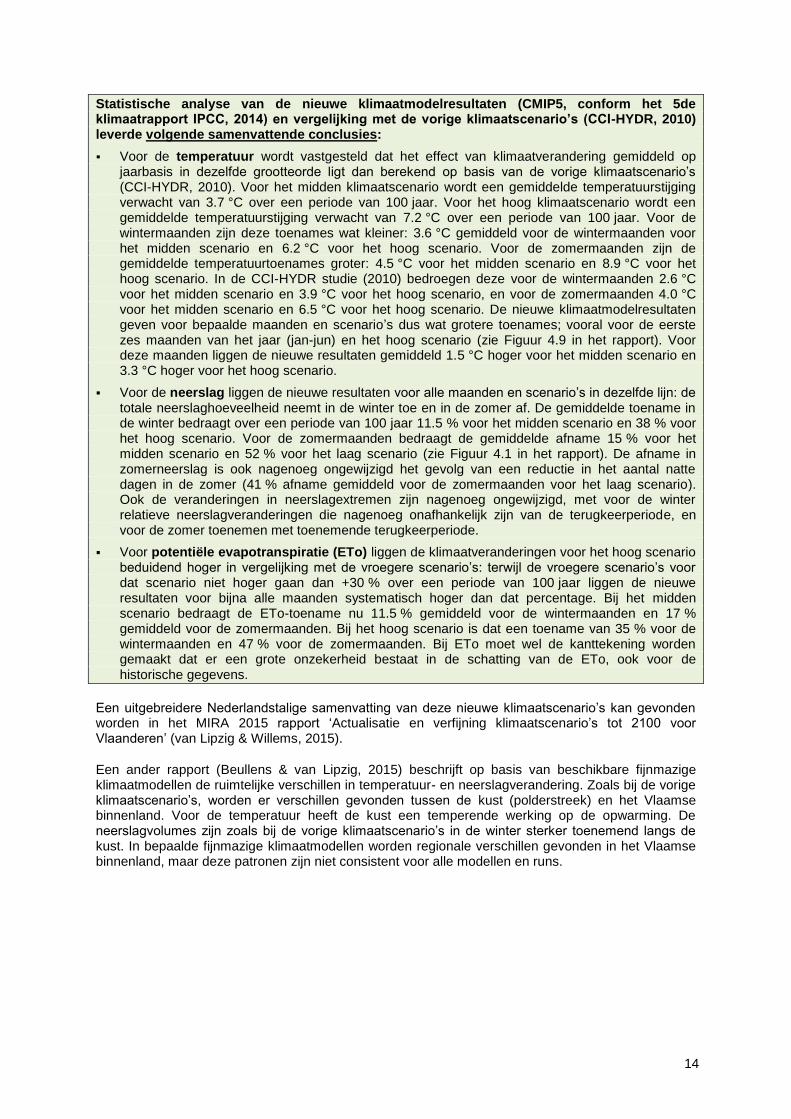
Statistische analyse van de nieuwe klimaatmodelresultaten (CMIP5, conform het 5de klimaatrapport IPCC, 2014) en vergelijking met de vorige klimaatscenario’s (CCI-HYDR, 2010) leverde volgende samenvattende conclusies:

Voor de temperatuur wordt vastgesteld dat het effect van klimaatverandering gemiddeld op jaarbasis in dezelfde grootteorde ligt dan berekend op basis van de vorige klimaatscenario’s (CCI-HYDR, 2010). Voor het midden klimaatscenario wordt een gemiddelde temperatuurstijging verwacht van 3.7 °C over een periode van 100 jaar. Voor het hoog klimaatscenario wordt een gemiddelde temperatuurstijging verwacht van 7.2 °C over een periode van 100 jaar. Voor de wintermaanden zijn deze toenames wat kleiner: 3.6 °C gemiddeld voor de wintermaanden voor het midden scenario en 6.2 °C voor het hoog scenario. Voor de zomermaanden zijn de gemiddelde temperatuurtoenames groter: 4.5 °C voor het midden scenario en 8.9 °C voor het hoog scenario. In de CCI-HYDR studie (2010) bedroegen deze voor de wintermaanden 2.6 °C voor het midden scenario en 3.9 °C voor het hoog scenario, en voor de zomermaanden 4.0 °C voor het midden scenario en 6.5 °C voor het hoog scenario. De nieuwe klimaatmodelresultaten geven voor bepaalde maanden en scenario’s dus wat grotere toenames; vooral voor de eerste zes maanden van het jaar (jan-jun) en het hoog scenario (zie Figuur 4.9 in het rapport). Voor deze maanden liggen de nieuwe resultaten gemiddeld 1.5 °C hoger voor het midden scenario en 3.3 °C hoger voor het hoog scenario.

Voor de neerslag liggen de nieuwe resultaten voor alle maanden en scenario’s in dezelfde lijn: de totale neerslaghoeveelheid neemt in de winter toe en in de zomer af. De gemiddelde toename in de winter bedraagt over een periode van 100 jaar 11.5 % voor het midden scenario en 38 % voor het hoog scenario. Voor de zomermaanden bedraagt de gemiddelde afname 15 % voor het midden scenario en 52 % voor het laag scenario (zie Figuur 4.1 in het rapport). De afname in zomerneerslag is ook nagenoeg ongewijzigd het gevolg van een reductie in het aantal natte dagen in de zomer (41 % afname gemiddeld voor de zomermaanden voor het laag scenario). Ook de veranderingen in neerslagextremen zijn nagenoeg ongewijzigd, met voor de winter relatieve neerslagveranderingen die nagenoeg onafhankelijk zijn van de terugkeerperiode, en voor de zomer toenemen met toenemende terugkeerperiode.

Voor potentiële evapotranspiratie (ETo) liggen de klimaatveranderingen voor het hoog scenario beduidend hoger in vergelijking met de vroegere scenario’s: terwijl de vroegere scenario’s voor dat scenario niet hoger gaan dan +30 % over een periode van 100 jaar liggen de nieuwe resultaten voor bijna alle maanden systematisch hoger dan dat percentage. Bij het midden scenario bedraagt de ETo-toename nu 11.5 % gemiddeld voor de wintermaanden en 17 % gemiddeld voor de zomermaanden. Bij het hoog scenario is dat een toename van 35 % voor de wintermaanden en 47 % voor de zomermaanden. Bij ETo moet wel de kanttekening worden gemaakt dat er een grote onzekerheid bestaat in de schatting van de ETo, ook voor de historische gegevens.

Een uitgebreidere Nederlandstalige samenvatting van deze nieuwe klimaatscenario’s kan gevonden worden in het MIRA 2015 rapport ‘Actualisatie en verfijning klimaatscenario’s tot 2100 voor Vlaanderen’ (van Lipzig & Willems, 2015).

Een ander rapport (Beullens & van Lipzig, 2015) beschrijft op basis van beschikbare fijnmazige klimaatmodellen de ruimtelijke verschillen in temperatuur- en neerslagverandering. Zoals bij de vorige klimaatscenario’s, worden er verschillen gevonden tussen de kust (polderstreek) en het Vlaamse binnenland. Voor de temperatuur heeft de kust een temperende werking op de opwarming. De neerslagvolumes zijn zoals bij de vorige klimaatscenario’s in de winter sterker toenemend langs de kust. In bepaalde fijnmazige klimaatmodellen worden regionale verschillen gevonden in het Vlaamse binnenland, maar deze patronen zijn niet consistent voor alle modellen en runs.

15

Het eindresultaat van de studie zijn aangepaste klimaatscenario’s, maar ook een aangepaste klimaatperturbatietool en bijhorende perturbatiefactoren. De klimaatperturbatietool wordt in de praktijk gebruikt om de invoer van hydrologische modellen aan te passen de hoog-midden-laag klimaatscenario’s. Omdat er geen significante wijziging werd vastgesteld in de perturbatie-factoren (klimaatveranderingssignaal) tussen de vorige CCI-HYDR scenario’s en de nieuwe, is er geen aanpassing gebeurd van de perturbatietool voor neerslag. Voor de temperatuur en vooral de ETo is er een significante wijziging in perturbatiefactoren voor het midden en hoog klimaatscenario. De perturbatietool werd hieraan aangepast. De aangepaste perturbatie-tool (versie 2014) is vrij beschikbaar op: http://www.kuleuven.be/hydr/CCI-HYDR.htm.

http://www.kuleuven.be/hydr/CCI-HYDR.htm

16

0 Introduction

This report presents the analysis of the new RCP based global climate model (GCM) simulations that became available recently in the database of the Coupled Model Intercomparison Project of the World Climate Research Programme - Phase 5 (CMIP5), and the related ongoing RCM simulations by the Coordinated Regional Climate Downscaling Experiment (CORDEX) for Europe. Also comparison is made with the higher resolution climate model runs that currently are in progress for Belgium. This analysis was jointly done for the division Operational Water Management of the Flemish Environment Agency (VMM), to develop tailored climate scenarios for hydrological and hydraulic impact analysis, and for the general environmental reporting (MIRA) 2015 by VMM.

1 New RCP based greenhouse concentration scenarios - introduction

1.1 SRES scenarios

The previous Assessment Report (4th Assessment Report, AR4) of the IPCC as well as the previous

CMIP runs and the previous Belgian CCI-HYDR based climate scenarios were based on climate model simulations where the external forcing is based on changes in greenhouse gasses (GHG) emissions, the so-called IPCC Special Report on Emissions Scenarios (SRES) A1, A2, B1, B2, A1B, etc. (Table 0.1; Nakicenovic et al., 2000). These were determined by driving functions such as demographic, socio-economic, technological and social development (Nakicenovic and Swart, 2000). Based on various overall scenarios, Nakicenovic and Swart (2000) developed 40 storylines that each describes a possible path. These possible paths span over wide intervals of human population, wealth, GHG concentrations and thus climate.

Table 0.1: SRES scenario summary

scenario description

A1 Fast growing economy, new/efficient technologies, population peak around mid-

century and decline thereafter. Three storyline subgroups: fossil intensive (A1FI),

fossil energy sources (A1T) and balanced use of all sources (A1B)

A2 Heterogeneous world, preservation of local identities, continuous population growth.

Economic/technological progress is more fragmented and slower than in other

scenarios

B1 Global population as in A1, services and information society, clean and resource

efficient technologies

B2 Global population as in A2 but slower evolution, intermediate economic

development, more diverse evolution in technology than in the A1 and B1 storylines

All the SRES scenarios are ‘baseline scenarios’ in the sense that they do not include any explicit climate policy (mitigation), although emission reduction may result from other environmental concerns that are taken into account in some scenarios. The CO2 emissions from the most frequently used SRES scenarios are shown on Source: Moss et al. (2008)

Figure 0.1 (coloured lines).

17

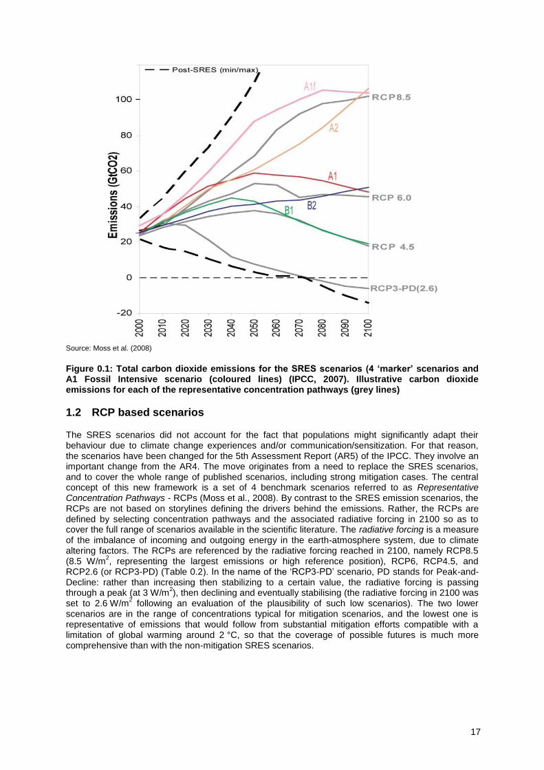
Source: Moss et al. (2008)

Figure 0.1: Total carbon dioxide emissions for the SRES scenarios (4 ‘marker’ scenarios and A1 Fossil Intensive scenario (coloured lines) (IPCC, 2007). Illustrative carbon dioxide emissions for each of the representative concentration pathways (grey lines)

1.2 RCP based scenarios

The SRES scenarios did not account for the fact that populations might significantly adapt their behaviour due to climate change experiences and/or communication/sensitization. For that reason, the scenarios have been changed for the 5th Assessment Report (AR5) of the IPCC. They involve an important change from the AR4. The move originates from a need to replace the SRES scenarios, and to cover the whole range of published scenarios, including strong mitigation cases. The central concept of this new framework is a set of 4 benchmark scenarios referred to as Representative Concentration Pathways - RCPs (Moss et al., 2008). By contrast to the SRES emission scenarios, the RCPs are not based on storylines defining the drivers behind the emissions. Rather, the RCPs are defined by selecting concentration pathways and the associated radiative forcing in 2100 so as to cover the full range of scenarios available in the scientific literature. The radiative forcing is a measure of the imbalance of incoming and outgoing energy in the earth-atmosphere system, due to climate altering factors. The RCPs are referenced by the radiative forcing reached in 2100, namely RCP8.5 (8.5 W/m

2, representing the largest emissions or high reference position), RCP6, RCP4.5, and

RCP2.6 (or RCP3-PD) (Table 0.2). In the name of the ‘RCP3-PD’ scenario, PD stands for Peak-and-Decline: rather than increasing then stabilizing to a certain value, the radiative forcing is passing through a peak (at 3 W/m

2), then declining and eventually stabilising (the radiative forcing in 2100 was

set to 2.6 W/m2 following an evaluation of the plausibility of such low scenarios). The two lower

scenarios are in the range of concentrations typical for mitigation scenarios, and the lowest one is representative of emissions that would follow from substantial mitigation efforts compatible with a limitation of global warming around 2 °C, so that the coverage of possible futures is much more comprehensive than with the non-mitigation SRES scenarios.

18

Table 0.2: RCP radiative forcing information

RCP8.5

rising radiative forcing pathway leading to 8.5 W/m² in 2100

RCP6

stabilization without overshoot pathway to 6 W/m² at stabilization after 2100

RCP4.5

stabilization without overshoot pathway to 4.5 W/m² at stabilization after 2100

RCP2.6

(RCP3-PD

peak in radiative forcing at 2.6 W/m² before 2100 and decline

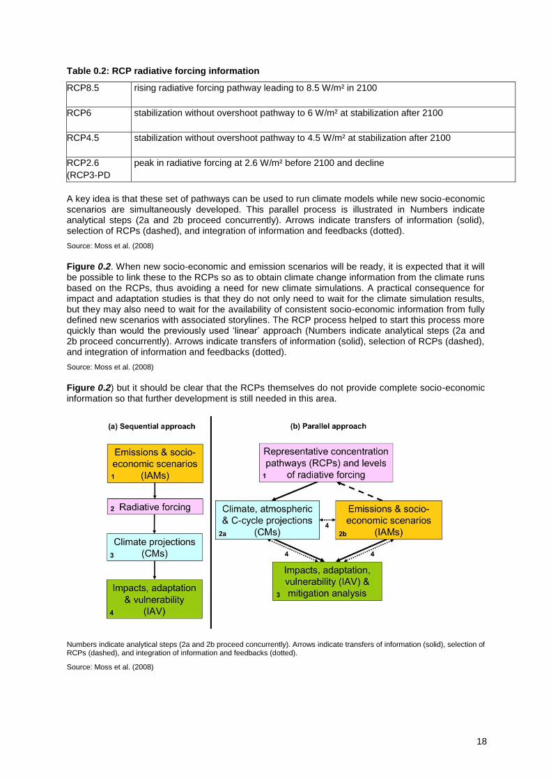
A key idea is that these set of pathways can be used to run climate models while new socio-economic scenarios are simultaneously developed. This parallel process is illustrated in Numbers indicate analytical steps (2a and 2b proceed concurrently). Arrows indicate transfers of information (solid), selection of RCPs (dashed), and integration of information and feedbacks (dotted).


Figure 0.2. When new socio-economic and emission scenarios will be ready, it is expected that it will be possible to link these to the RCPs so as to obtain climate change information from the climate runs based on the RCPs, thus avoiding a need for new climate simulations. A practical consequence for impact and adaptation studies is that they do not only need to wait for the climate simulation results, but they may also need to wait for the availability of consistent socio-economic information from fully defined new scenarios with associated storylines. The RCP process helped to start this process more quickly than would the previously used ‘linear’ approach (Numbers indicate analytical steps (2a and 2b proceed concurrently). Arrows indicate transfers of information (solid), selection of RCPs (dashed), and integration of information and feedbacks (dotted).


Figure 0.2) but it should be clear that the RCPs themselves do not provide complete socio-economic information so that further development is still needed in this area.

Numbers indicate analytical steps (2a and 2b proceed concurrently). Arrows indicate transfers of information (solid), selection of RCPs (dashed), and integration of information and feedbacks (dotted).


19

Figure 0.2: Approaches to the development of climate forcing scenarios: (a) previous sequential approach for the SRES emission scenarios; (b) parallel approach of the RCP based scenarios

Dashed lines around climate-carbon cycle coupling methods indicate that not all models are coupled.

Source: Ward et al. (2011)

Figure 0.3 shows the main differences in the processes involved when applying SRES emission scenarios versus AR5 RCP based scenarios. The figure is based on the main stages in developing a model of the hydrological impacts from climate change as described by Ward et al. (2011). The SRES scenarios worked ‘forward’ from socioeconomic projections to radiative forcings (sequential approach; Numbers indicate analytical steps (2a and 2b proceed concurrently). Arrows indicate transfers of information (solid), selection of RCPs (dashed), and integration of information and feedbacks (dotted).


Figure 0.2). This made it easy to get bogged down in questioning the socioeconomic, technological, and physical assumptions of the scenarios. In contrast, the RCPs are intended to work backwards from assuming forcings of magnitude to the wide range of circumstances that might result in such forcings. This means that the RCPs are ‘agnostic’ to the specifics of the socioeconomic projections; no matter how socioeconomic, politics, and technology are going to evolve during the 21

st century.

The higher steps in Dashed lines around climate-carbon cycle coupling methods indicate that not all models are coupled.


Figure 0.3 of emission scenario definition and carbon cycle modelling thus are eliminated from the AR5 scenario definition. In this report, climate forcing scenarios is used as a common term for both the SRES emissions and AR5 RCP based scenarios.

Dashed lines around climate-carbon cycle coupling methods indicate that not all models are coupled.


20

Figure 0.3: Simplified chart of the main processes involved in modelling hydrological impacts from climate change

1.3 Practical use of the climate scenarios for decision making

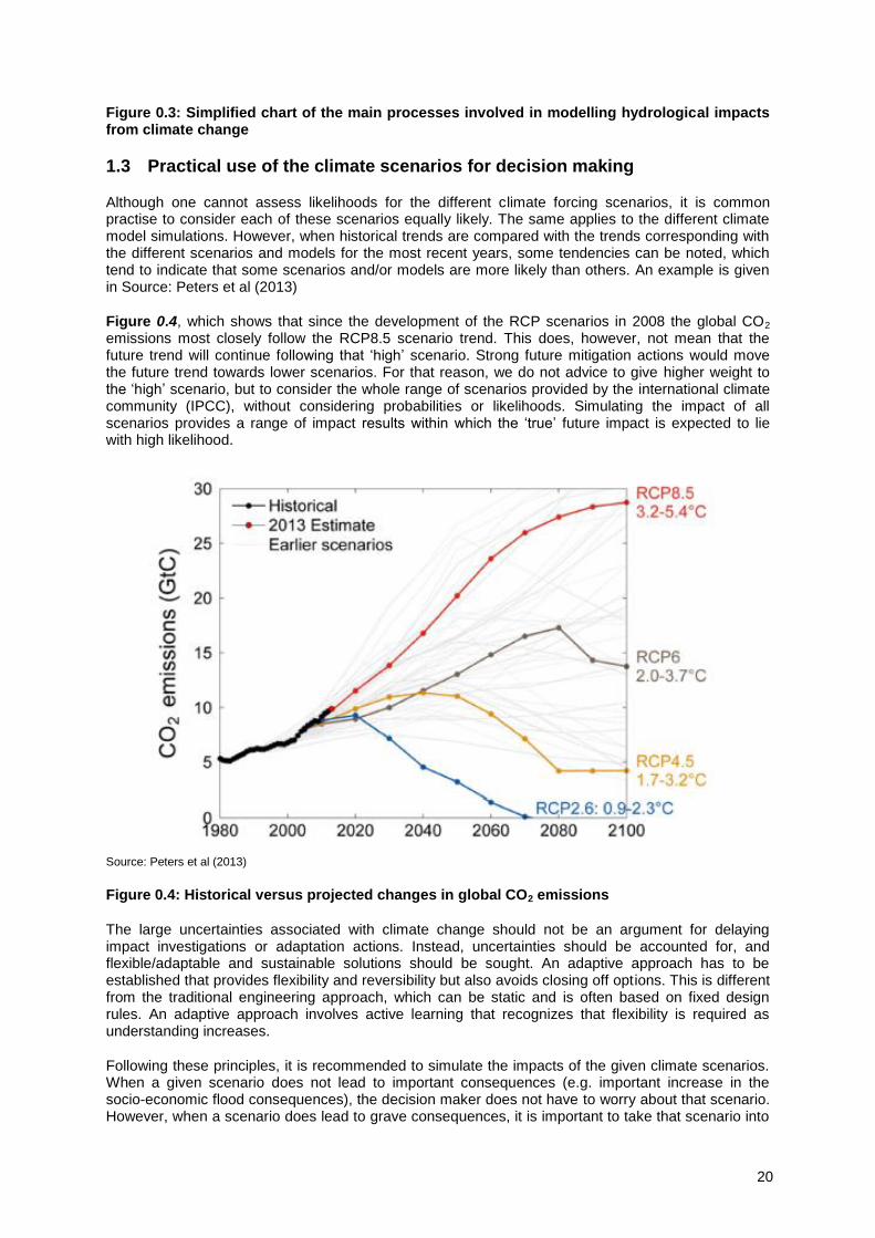
Although one cannot assess likelihoods for the different climate forcing scenarios, it is common practise to consider each of these scenarios equally likely. The same applies to the different climate model simulations. However, when historical trends are compared with the trends corresponding with the different scenarios and models for the most recent years, some tendencies can be noted, which tend to indicate that some scenarios and/or models are more likely than others. An example is given in Source: Peters et al (2013)

Figure 0.4, which shows that since the development of the RCP scenarios in 2008 the global CO2 emissions most closely follow the RCP8.5 scenario trend. This does, however, not mean that the future trend will continue following that ‘high’ scenario. Strong future mitigation actions would move the future trend towards lower scenarios. For that reason, we do not advice to give higher weight to the ‘high’ scenario, but to consider the whole range of scenarios provided by the international climate community (IPCC), without considering probabilities or likelihoods. Simulating the impact of all scenarios provides a range of impact results within which the ‘true’ future impact is expected to lie with high likelihood.

Source: Peters et al (2013)

Figure 0.4: Historical versus projected changes in global CO2 emissions

The large uncertainties associated with climate change should not be an argument for delaying impact investigations or adaptation actions. Instead, uncertainties should be accounted for, and flexible/adaptable and sustainable solutions should be sought. An adaptive approach has to be established that provides flexibility and reversibility but also avoids closing off options. This is different from the traditional engineering approach, which can be static and is often based on fixed design rules. An adaptive approach involves active learning that recognizes that flexibility is required as understanding increases.

Following these principles, it is recommended to simulate the impacts of the given climate scenarios. When a given scenario does not lead to important consequences (e.g. important increase in the socio-economic flood consequences), the decision maker does not have to worry about that scenario. However, when a scenario does lead to grave consequences, it is important to take that scenario into

21

account in the decision making; according to the ‘precautionary principle’. Depending on the severity of the impacts and the time/possibilities one has to adapt (taking into account that the future climate change trends will be gradual in time), one can decide to delay adaptation actions but recommend for careful follow-up of the future climate trends such that the adaptation strategy can be upgraded gradually in time, or one can already decide to start taking adaptation actions now. Whichever adaptation strategy is selected or whichever decisions are presently taken as part of the regular management programme, one has to check whether the decisions are efficient and effective under all climate scenarios. One has to avoid taking decisions that later on (under one of the future scenarios) may turn out to be ineffective and that inhibit the decision to be (relatively easily) reversed. So, one has to avoid irreversibility or closing off options.

22

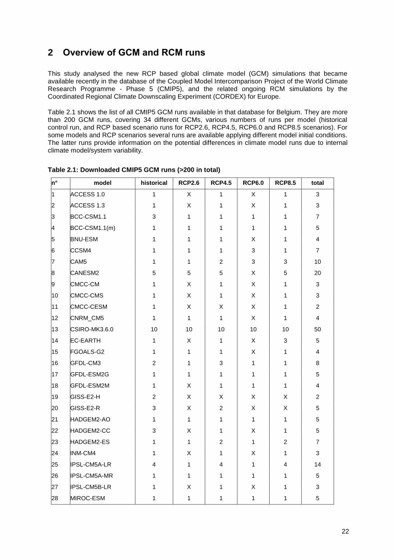
2 Overview of GCM and RCM runs

This study analysed the new RCP based global climate model (GCM) simulations that became available recently in the database of the Coupled Model Intercomparison Project of the World Climate Research Programme - Phase 5 (CMIP5), and the related ongoing RCM simulations by the Coordinated Regional Climate Downscaling Experiment (CORDEX) for Europe.

Table 2.1 shows the list of all CMIP5 GCM runs available in that database for Belgium. They are more than 200 GCM runs, covering 34 different GCMs, various numbers of runs per model (historical control run, and RCP based scenario runs for RCP2.6, RCP4.5, RCP6.0 and RCP8.5 scenarios). For some models and RCP scenarios several runs are available applying different model initial conditions. The latter runs provide information on the potential differences in climate model runs due to internal climate model/system variability.

Table 2.1: Downloaded CMIP5 GCM runs (>200 in total)

n° model historical RCP2.6 RCP4.5 RCP6.0 RCP8.5 total

1 ACCESS 1.0 1 X 1 X 1 3

2 ACCESS 1.3 1 X 1 X 1 3

3 BCC-CSM1.1 3 1 1 1 1 7

4 BCC-CSM1.1(m) 1 1 1 1 1 5

5 BNU-ESM 1 1 1 X 1 4

6 CCSM4 1 1 1 3 1 7

7 CAM5 1 1 2 3 3 10

8 CANESM2 5 5 5 X 5 20

9 CMCC-CM 1 X 1 X 1 3

10 CMCC-CMS 1 X 1 X 1 3

11 CMCC-CESM 1 X X X 1 2

12 CNRM_CM5 1 1 1 X 1 4

13 CSIRO-MK3.6.0 10 10 10 10 10 50

14 EC-EARTH 1 X 1 X 3 5

15 FGOALS-G2 1 1 1 X 1 4

16 GFDL-CM3 2 1 3 1 1 8

17 GFDL-ESM2G 1 1 1 1 1 5

18 GFDL-ESM2M 1 X 1 1 1 4

19 GISS-E2-H 2 X X X X 2

20 GISS-E2-R 3 X 2 X X 5

21 HADGEM2-AO 1 1 1 1 1 5

22 HADGEM2-CC 3 X 1 X 1 5

23 HADGEM2-ES 1 1 2 1 2 7

24 INM-CM4 1 X 1 X 1 3

25 IPSL-CM5A-LR 4 1 4 1 4 14

26 IPSL-CM5A-MR 1 1 1 1 1 5

27 IPSL-CM5B-LR 1 X 1 X 1 3

28 MIROC-ESM 1 1 1 1 1 5

23

29 MIROC-ESM-CHEM 1 1 1 1 1 5

30 MIROC5 3 2 1 1 3 10

31 MPI-ESM_LR 1 1 1 X 1 4

32 MPI-ESM_MR 1 1 1 X 1 4

33 MRI-CGCM3 1 1 1 1 1 5

34 NORESM1-M 3 1 1 1 1 7

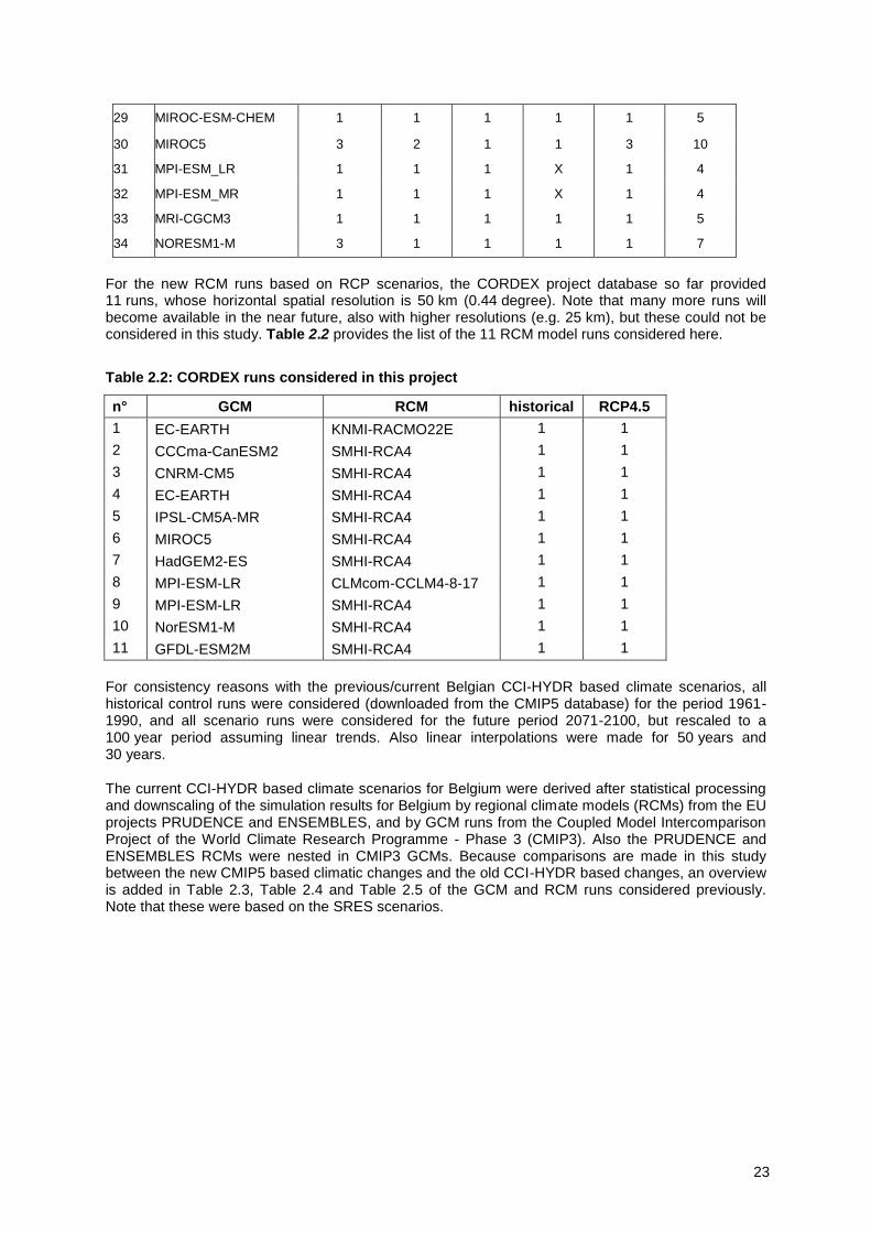
For the new RCM runs based on RCP scenarios, the CORDEX project database so far provided 11 runs, whose horizontal spatial resolution is 50 km (0.44 degree). Note that many more runs will become available in the near future, also with higher resolutions (e.g. 25 km), but these could not be considered in this study. Table 2.2 provides the list of the 11 RCM model runs considered here.

Table 2.2: CORDEX runs considered in this project

n° GCM RCM historical RCP4.5

1 EC-EARTH KNMI-RACMO22E 1 1

2 CCCma-CanESM2 SMHI-RCA4 1 1

3 CNRM-CM5 SMHI-RCA4 1 1

4 EC-EARTH SMHI-RCA4 1 1

5 IPSL-CM5A-MR SMHI-RCA4 1 1

6 MIROC5 SMHI-RCA4 1 1

7 HadGEM2-ES SMHI-RCA4 1 1

8 MPI-ESM-LR CLMcom-CCLM4-8-17 1 1

9 MPI-ESM-LR SMHI-RCA4 1 1

10 NorESM1-M SMHI-RCA4 1 1

11 GFDL-ESM2M SMHI-RCA4 1 1

For consistency reasons with the previous/current Belgian CCI-HYDR based climate scenarios, all historical control runs were considered (downloaded from the CMIP5 database) for the period 1961-1990, and all scenario runs were considered for the future period 2071-2100, but rescaled to a 100 year period assuming linear trends. Also linear interpolations were made for 50 years and 30 years.

The current CCI-HYDR based climate scenarios for Belgium were derived after statistical processing and downscaling of the simulation results for Belgium by regional climate models (RCMs) from the EU projects PRUDENCE and ENSEMBLES, and by GCM runs from the Coupled Model Intercomparison Project of the World Climate Research Programme - Phase 3 (CMIP3). Also the PRUDENCE and ENSEMBLES RCMs were nested in CMIP3 GCMs. Because comparisons are made in this study between the new CMIP5 based climatic changes and the old CCI-HYDR based changes, an overview is added in Table 2.3, Table 2.4 and Table 2.5 of the GCM and RCM runs considered previously. Note that these were based on the SRES scenarios.

24

Table 2.3: CMIP3 GCM runs considered for the CCI-HYDR based scenarios

n° model control A2 A1B B1

1 CCCma-CGCM3 (T47) 1 2 2 2

2 CCCma-CGCM3 (T4)63 1 X 1 1

3 CNRM-CM3 1 X 1 1

4 CSIRO-Mk3.0 1 1 1 1

5 CSIRO-Mk3.5 1 1 1 1

6 MIUB-ECHO-G 1 3 3 3

7 GFDL-CM2.0 1 1 1 1

8 GFDL-CM2.1 1 1 X 1

9 IPSL-CM4 1 1 1 1

10 MIROC3.2 hires 1 X 1 X

11 MIROC3.2 medres 1 2 2 X

12 MRI-CGCM2.3.2 1 5 5 5

13 NCAR-CCSM3 1 1 2 1

14 NCAR-PCM 1 X X 1

15 MPI-ECHAM5 1 1 X X

16 IAP-FGOALS 1 X 2 2

25

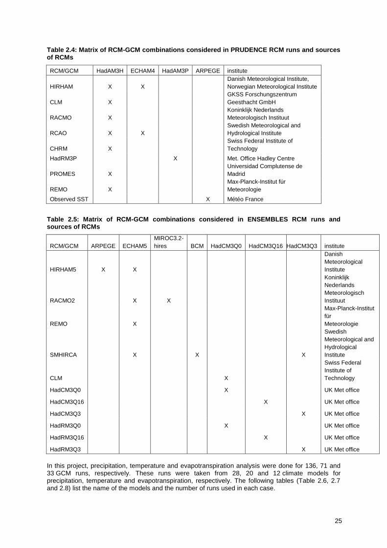
Table 2.4: Matrix of RCM-GCM combinations considered in PRUDENCE RCM runs and sources of RCMs

RCM/GCM HadAM3H ECHAM4 HadAM3P ARPEGE institute

HIRHAM X X

Danish Meteorological Institute,

Norwegian Meteorological Institute

CLM X

GKSS Forschungszentrum

Geesthacht GmbH

RACMO X

Koninklijk Nederlands

Meteorologisch Instituut

RCAO X X

Swedish Meteorological and

Hydrological Institute

CHRM X

Swiss Federal Institute of

Technology

HadRM3P

X

Met. Office Hadley Centre

PROMES X

Universidad Complutense de

Madrid

REMO X

Max-Planck-Institut für

Meteorologie

Observed SST

X Météo France

Table 2.5: Matrix of RCM-GCM combinations considered in ENSEMBLES RCM runs and sources of RCMs

RCM/GCM ARPEGE ECHAM5

MIROC3.2-

hires BCM HadCM3Q0 HadCM3Q16 HadCM3Q3 institute

HIRHAM5 X X

Danish

Meteorological

Institute

RACMO2

X X

Koninklijk

Nederlands

Meteorologisch

Instituut

REMO

X

Max-Planck-Institut

für

Meteorologie

SMHIRCA

X

X

X

Swedish

Meteorological and

Hydrological

Institute

CLM

X

Swiss Federal

Institute of

Technology

HadCM3Q0

X

UK Met office

HadCM3Q16

X

UK Met office

HadCM3Q3

X UK Met office

HadRM3Q0

X

UK Met office

HadRM3Q16

X

UK Met office

HadRM3Q3

X UK Met office

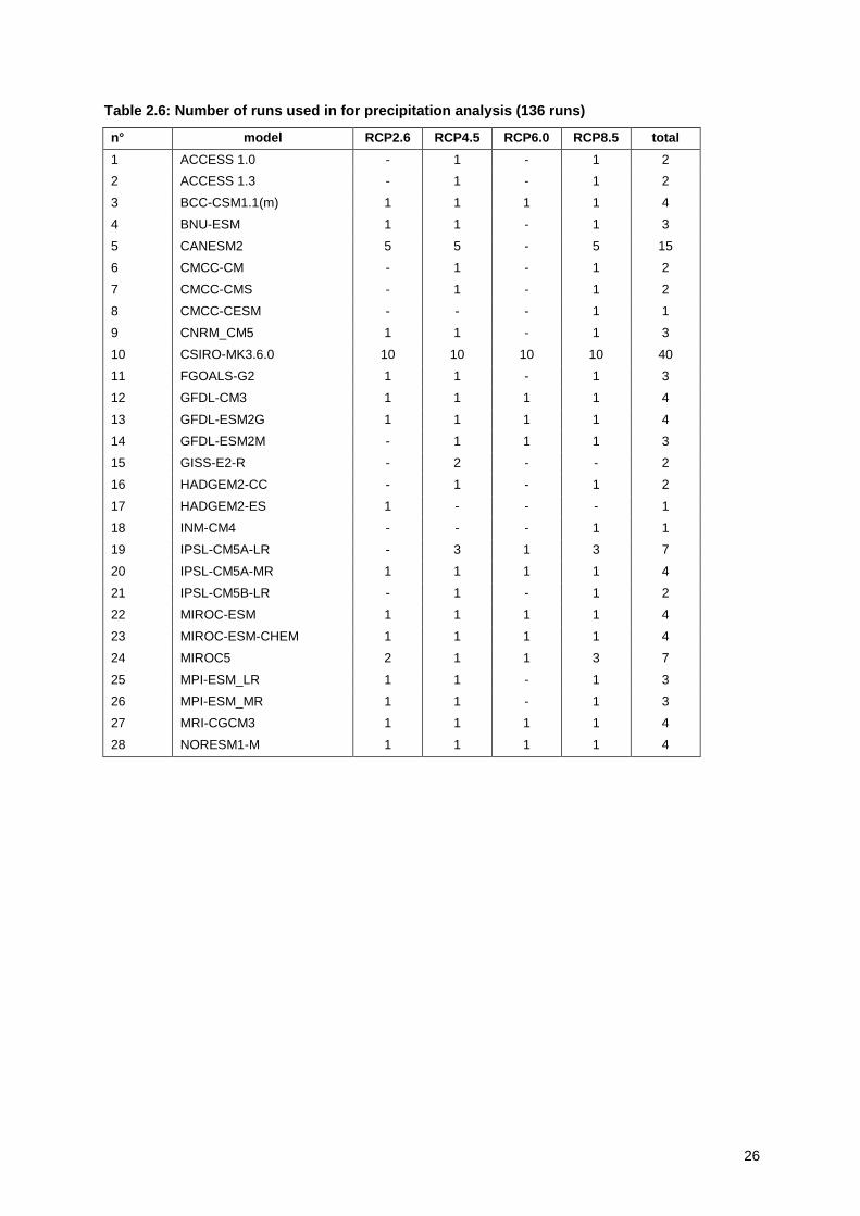
In this project, precipitation, temperature and evapotranspiration analysis were done for 136, 71 and 33 GCM runs, respectively. These runs were taken from 28, 20 and 12 climate models for precipitation, temperature and evapotranspiration, respectively. The following tables (Table 2.6, 2.7 and 2.8) list the name of the models and the number of runs used in each case.

26

Table 2.6: Number of runs used in for precipitation analysis (136 runs)

n° model RCP2.6 RCP4.5 RCP6.0 RCP8.5 total

1 ACCESS 1.0 - 1 - 1 2

2 ACCESS 1.3 - 1 - 1 2

3 BCC-CSM1.1(m) 1 1 1 1 4

4 BNU-ESM 1 1 - 1 3

5 CANESM2 5 5 - 5 15

6 CMCC-CM - 1 - 1 2

7 CMCC-CMS - 1 - 1 2

8 CMCC-CESM - - - 1 1

9 CNRM_CM5 1 1 - 1 3

10 CSIRO-MK3.6.0 10 10 10 10 40

11 FGOALS-G2 1 1 - 1 3

12 GFDL-CM3 1 1 1 1 4

13 GFDL-ESM2G 1 1 1 1 4

14 GFDL-ESM2M - 1 1 1 3

15 GISS-E2-R - 2 - - 2

16 HADGEM2-CC - 1 - 1 2

17 HADGEM2-ES 1 - - - 1

18 INM-CM4 - - - 1 1

19 IPSL-CM5A-LR - 3 1 3 7

20 IPSL-CM5A-MR 1 1 1 1 4

21 IPSL-CM5B-LR - 1 - 1 2

22 MIROC-ESM 1 1 1 1 4

23 MIROC-ESM-CHEM 1 1 1 1 4

24 MIROC5 2 1 1 3 7

25 MPI-ESM_LR 1 1 - 1 3

26 MPI-ESM_MR 1 1 - 1 3

27 MRI-CGCM3 1 1 1 1 4

28 NORESM1-M 1 1 1 1 4

27

Table 2.7: Number of runs used in for temperature analysis (71 runs)


1 BNU-ESM 1 1 - 1 3

2 CANESM2 5 5 - 5 15

3 CMCC-CMS - 1 - 1 2

4 CMCC-CESM - - - 1 1

5 CNRM_CM5 1 1 - 1 3

6 CSIRO-MK3.6.0 1 1 2 2 6

7 GFDL-ESM2G 1 1 1 1 4

8 GFDL-ESM2M - 1 1 1 3

9 GISS-E2-R - 2 - - 2

10 HADGEM2-CC - 1 - 1 2

11 HADGEM2-ES 1 1 - - 2

12 IPSL-CM5A-LR - 2 1 2 5

13 IPSL-CM5A-MR 1 1 1 1 4

14 IPSL-CM5B-LR - 1 - 1 2

15 MIROC-ESM 1 1 1 1 4

16 MIROC5 - - 1 3 4

17 MPI-ESM_LR - - - 1 1

18 MPI-ESM_MR 1 1 - 1 3

19 MRI-CGCM3 - 1 1 1 3

20 NORESM1-M - - 1 1 2

Table 2.8: Number of runs used in for potential evapotranspiration analysis (33 runs)


1 BNU-ESM 1 1 - - 2

2 CNRM_CM5 - 1 - 1 2

3 GFDL-CM3 1

1 1 3

4 GFDL-ESM2G 1 1 1 1 4

5 GFDL-ESM2M - 1 1 1 3

6 HADGEM2-CC - 1 - - 1

7 INM-CM4 - 1 - - 1

8 IPSL-CM5A-LR 1 - 1 1 3

9 IPSL-CM5A-MR 1 - 1 1 3

10 MIROC-ESM 1 1 1 1 4

11 MIROC-ESM-CHEM 1 1 1 1 4

12 MRI-CGCM3 1 1 - 1 3

28

3 Statistical analysis of CMIP5 GCM runs

The results of the new CMIP5 GCM results were statistically processed and evaluated by comparison with the historical observations at Uccle. This is done for the GCM grid cell covering that station. After this validation based on the GCM historical control runs, the GCM scenario runs were statistically processed and results (simulated climate changes) were analysed for precipitation, temperature, potential evapotranspiration (ETo) and wind speed.

For precipitation, temperature and wind speed, the climate model results are considered as such. This is different for ETo. Although the climate models provide ETo as outputs, they are not that reliable, and inconsistent with the common method (Penman-Monteith or the more specific Bultot method) applied in Belgium for the computation of ETo. Section 3.1 first explains the method applied to compute the ETo from different meteorological variables computed by the climate models. This is followed by the validation of the CMIP5 climate model control runs for Belgium in Section 3.2. The analysis of the climate changes is reported in Section 3.3.

3.1 ETo calculation

The ETo was calculated consistently with the CCI-HYDR climate scenarios using the Bultot method (Bultot, 1983), which is the standard method for Belgium as developed and applied by the Royal Meteorological Institute of Belgium (RMI).

Potential evapotranspiration of a natural cover is the amount of water vapor that could be generated from a free water surface that receives the same amount of energy and transforming this energy according to the same Bowen ratio as the natural cover under consideration (Penman, 1948; Bultot et al., 1983; Gellens-Meulenberghs and Gellens, 1992).

Following the Penman method, the evaporation 0E (mm/day) of a free water surface is computed as

follows:

))((/*0

0

e- u LQ E

where:

p

dT

d

LKQ

T

000662.0

-)-1( *

s0

*

0

with:

Q0* : total radiation balance (J/(cm

2day))

Ks : global solar radiation (J/(cm2day))

L * : net terrestrial radiation (J/(cm

2day))

L : vaporization latent heat of water (10-4

J/kg)

: psychrometric coefficient (hPa/K) p : mean annual atmospheric pressure (hPa) u : mean daily wind speed at 2m (km/h) ε - e : saturation deficit (hPa)

α0 : free water surface albedoThe parameters and can be determined with

evaporation measurements and their values are known for 11 Belgian stations from the research by

Bultot et al. (1983). As in the CCI-HYDR study, the following values are used: 205.0 and

028.0 .

29

The free water surface albedo is calculated using:

4.00 )07.0(07.0 Ir-A

where A is the albedo of the free water surface under clear sky (Table 3.1) and Ir is the relative

insolation, while the net terrestrial radiation *L is given by the Monteith formula (Monteith, 1973):

)))-1( 1()(-1( 24* IrcebaTL

In this equation, 1428100422.2 hKJcm is the Stefan-Botzmann constant, e the water

vapour pressure in hPa and T the air temperature in degrees Kelvin. The parameters a, b and c can be determined by measurements on radiation variables (Bultot et al., 1983) and are location specific. Their seasonal values for the RMI location at Uccle are summarized in Table 3.2.

Table 3.1: Monthly values of the free water surface albedo under clear sky as a function of relative insolation at 50

o latitude

Ir jan feb mar apr may jun jul aug sep oct nov

0.0 0.07 0.07 0.07 0.07 0.07 0.07 0.07 0.07 0.07 0.07 0.07

0.1 0.114 0.098 0.082 0.074 0.07 0.07 0.07 0.066 0.074 0.086 0.106

0.2 0.128 0.107 0.086 0.075 0.07 0.07 0.07 0.065 0.075 0.091 0.117

0.4 0.146 0.119 0.091 0.077 0.07 0.07 0.07 0.063 0.077 0.098 0.132

0.6 0.16 0.127 0.094 0.078 0.07 0.07 0.07 0.062 0.078 0.103 0.143

0.8 0.171 0.134 0.097 0.079 0.07 0.07 0.07 0.061 0.079 0.107 0.152

1.0 0.18 0.14 0.1 0.08 0.07 0.07 0.07 0.06 0.08 0.11 0.16

Table 3.2: Seasonal radiation parameters for the Bultot method

a b c

winter 0.4117 0.1604 0.1498

spring 0.4599 0.1006 0.2397

summer 0.6869 0.0293 0.1741

autumn 0.5824 0.0718 0.1472

Saturated vapour pressure (ε) is given by:

2

minmax TT

where:

)3.237

27.17exp(6108.0

max

max

max

T

TT

)3.237

27.17exp(6108.0

min

min

min

T

TT

30

Actual vapour pressure (e) is given by

100

RHe

where RH is mean relative humidity (%).

The potential evapotranspiration iETo (mm/day) of a natural cover i is given by:

.0ii EfETo

In this equation, f is a transfer coefficient given by:

*s0

*s

)1(

)1(

L-K-

L-K-f

i

where iα denotes the albedo of the natural cover surface. From the previous analysis it becomes

evident that the calculation of ETo from the output of the climatic model simulations, involves the following variables (in parentheses are the code names in the CMIP5 database):

Mean Sea Level Pressure (psl)

Surface Downwelling Shortwave Radiation (rsds)

Mean 2-meter Air Temperature (tas)

Maximum 2-meter Air Temperature (tasmax)

Minimum 2-meter Air Temperature (tasmin)

Mean 10-meter Wind Speed (sfcWind)

Near-Surface Relative Humidity (rhs)

These calculations were performed at the daily time step to obtain daily ETo time series.

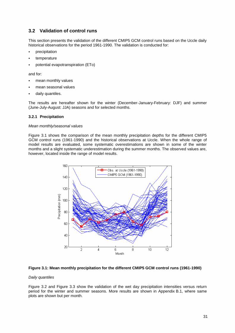
31

3.2 Validation of control runs

This section presents the validation of the different CMIP5 GCM control runs based on the Uccle daily historical observations for the period 1961-1990. The validation is conducted for:

precipitation

temperature

potential evapotranspiration (ETo)

and for:

mean monthly values

mean seasonal values

daily quantiles.

The results are hereafter shown for the winter (December-January-February: DJF) and summer (June-July-August: JJA) seasons and for selected months.

3.2.1 Precipitation

Mean monthly/seasonal values

Figure 3.1 shows the comparison of the mean monthly precipitation depths for the different CMIP5 GCM control runs (1961-1990) and the historical observations at Uccle. When the whole range of model results are evaluated, some systematic overestimations are shown in some of the winter months and a slight systematic underestimation during the summer months. The observed values are, however, located inside the range of model results.

Figure 3.1: Mean monthly precipitation for the different CMIP5 GCM control runs (1961-1990)

Daily quantiles

Figure 3.2 and Figure 3.3 show the validation of the wet day precipitation intensities versus return period for the winter and summer seasons. More results are shown in Appendix B.1, where same plots are shown but per month.

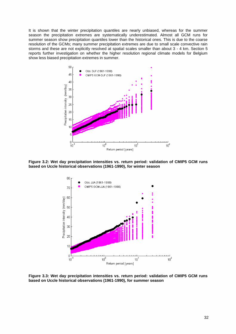
32

It is shown that the winter precipitation quantiles are nearly unbiased, whereas for the summer season the precipitation extremes are systematically underestimated. Almost all GCM runs for summer season show precipitation quantiles lower than the historical ones. This is due to the coarse resolution of the GCMs; many summer precipitation extremes are due to small scale convective rain storms and these are not explicitly resolved at spatial scales smaller than about 3 - 4 km. Section 5 reports further investigation on whether the higher resolution regional climate models for Belgium show less biased precipitation extremes in summer.

Figure 3.2: Wet day precipitation intensities vs. return period: validation of CMIP5 GCM runs based on Uccle historical observations (1961-1990), for winter season

Figure 3.3: Wet day precipitation intensities vs. return period: validation of CMIP5 GCM runs based on Uccle historical observations (1961-1990), for summer season

33

3.2.2 Temperature


Mean monthly values of temperature for GCM control runs and the values observed at Uccle station are shown in Figure 3.4. As one can see, all of the climate models can capture the inter-annual variation of air temperature. The observed and climate models’ simulated air temperature follow similar pattern. In terms of magnitude, most of the climate model runs systematically overestimate the mean monthly temperature values.

Figure 3.4: Mean monthly temperature for the different CMIP5 GCM control runs (1961-1990)

Daily quantiles

Variations of high temperature extremes versus winter and summer seasons are illustrated in Figure 3.5. Similar to the winter precipitation quantiles, daily temperature quantiles for winter season are unbiased. Wider range of estimated summer temperature by the climate models compared with winter temperature indicates lower capabilities of climate models for estimating summer temperature. It can be inferred from the results that the majority of the models overestimated summer temperature.

See again Appendix B for the detailed results per month.

Figure 3.5: Temperature vs. return period: validation of CMIP5 GCM runs based on Uccle historical observations (1961-1990), for winter and summer season

34

3.2.3 ETo


Mean monthly values of ETo for GCM control runs and the values observed at Uccle station are shown in Figure 3.6. As one can see, all of the climate models can capture the inter-annual variation of ETo. The observed and climate models’ simulated ETo follow similar pattern. In terms of magnitude, most of the climate model runs systematically overestimate the mean monthly ETo values especially for summer.

Figure 3.6: Mean monthly ETo for the different CMIP5 GCM control runs (1961-1990)

Daily quantiles

Figure 3.7 shows the variation of daily ETo for winter and summer seasons respectively. It is found that summer ETo values are overestimated by almost all climate models, while half of the models overestimate winter ETo values. Therefore, the estimated summer ETo values by most of the models are unreliable for use in hydrological impact of climate change. Given that the summer air temperature results in previous section show less biased results, the overestimations of summer ETo must be due to one of the other meteorological variables such as radiation, wind speed, humidity, and air temperature. Air temperature indeed explains only part of the ETo variation. For this reason, more efforts are necessary to understand which meteorological parameters are responsible for the overestimation of ETo especially for the summer season. We included sensitivity analysis for the climate model with the highest ETo change in Section 4.

35

Figure 3.7: Evapotranspiration vs. return period: validation of CMIP5 GCM runs based on Uccle historical observations (1961-1990), for winter and summer season

3.2.4 Conclusions

From the validation of the CMIP5 GCM control runs for precipitation, temperature and ETo, for mean monthly/seasonal values and daily quantiles, we conclude that:

CMIP5 GCM control runs for mean monthly precipitation show systematic over- and underestimations for winter and summer months respectively.

Precipitation extremes are systematically underestimated during summer months.

Temperature is more accurately simulated than precipitation; but slight overestimations of temperature are noted.

Daily evapotranspiration extremes are systematically overestimated during summer season, whereas both over- and underestimations are observed for winter season. This must be due to systematic differences in other meteorological variable(s) than air temperature, which needs further investigation.

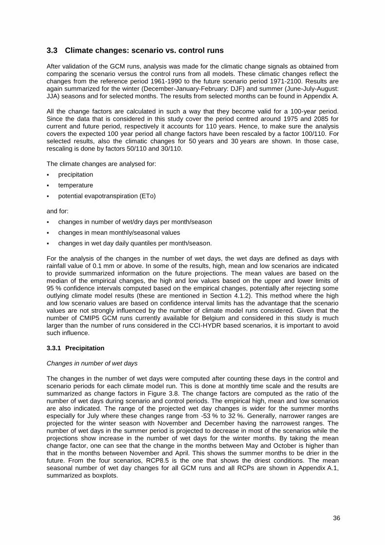
36

3.3 Climate changes: scenario vs. control runs

After validation of the GCM runs, analysis was made for the climatic change signals as obtained from comparing the scenario versus the control runs from all models. These climatic changes reflect the changes from the reference period 1961-1990 to the future scenario period 1971-2100. Results are again summarized for the winter (December-January-February: DJF) and summer (June-July-August: JJA) seasons and for selected months. The results from selected months can be found in Appendix A.

All the change factors are calculated in such a way that they become valid for a 100-year period. Since the data that is considered in this study cover the period centred around 1975 and 2085 for current and future period, respectively it accounts for 110 years. Hence, to make sure the analysis covers the expected 100 year period all change factors have been rescaled by a factor 100/110. For selected results, also the climatic changes for 50 years and 30 years are shown. In those case, rescaling is done by factors 50/110 and 30/110.

The climate changes are analysed for:

precipitation

temperature

potential evapotranspiration (ETo)

and for:

changes in number of wet/dry days per month/season

changes in mean monthly/seasonal values

changes in wet day daily quantiles per month/season.

For the analysis of the changes in the number of wet days, the wet days are defined as days with rainfall value of 0.1 mm or above. In some of the results, high, mean and low scenarios are indicated to provide summarized information on the future projections. The mean values are based on the median of the empirical changes, the high and low values based on the upper and lower limits of 95 % confidence intervals computed based on the empirical changes, potentially after rejecting some outlying climate model results (these are mentioned in Section 4.1.2). This method where the high and low scenario values are based on confidence interval limits has the advantage that the scenario values are not strongly influenced by the number of climate model runs considered. Given that the number of CMIP5 GCM runs currently available for Belgium and considered in this study is much larger than the number of runs considered in the CCI-HYDR based scenarios, it is important to avoid such influence.

3.3.1 Precipitation

Changes in number of wet days

The changes in the number of wet days were computed after counting these days in the control and scenario periods for each climate model run. This is done at monthly time scale and the results are summarized as change factors in Figure 3.8. The change factors are computed as the ratio of the number of wet days during scenario and control periods. The empirical high, mean and low scenarios are also indicated. The range of the projected wet day changes is wider for the summer months especially for July where these changes range from -53 % to 32 %. Generally, narrower ranges are projected for the winter season with November and December having the narrowest ranges. The number of wet days in the summer period is projected to decrease in most of the scenarios while the projections show increase in the number of wet days for the winter months. By taking the mean change factor, one can see that the change in the months between May and October is higher than that in the months between November and April. This shows the summer months to be drier in the future. From the four scenarios, RCP8.5 is the one that shows the driest conditions. The mean seasonal number of wet day changes for all GCM runs and all RCPs are shown in Appendix A.1, summarized as boxplots.

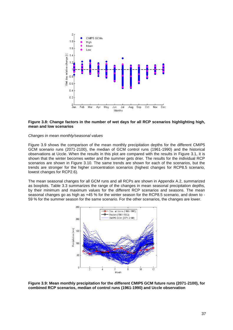
37

Figure 3.8: Change factors in the number of wet days for all RCP scenarios highlighting high, mean and low scenarios

Changes in mean monthly/seasonal values

Figure 3.9 shows the comparison of the mean monthly precipitation depths for the different CMIP5 GCM scenario runs (2071-2100), the median of GCM control runs (1961-1990) and the historical observations at Uccle. When the results in this plot are compared with the results in Figure 3.1, it is shown that the winter becomes wetter and the summer gets drier. The results for the individual RCP scenarios are shown in Figure 3.10. The same trends are shown for each of the scenarios, but the trends are stronger for the higher concentration scenarios (highest changes for RCP8.5 scenario, lowest changes for RCP2.6).

The mean seasonal changes for all GCM runs and all RCPs are shown in Appendix A.2, summarized as boxplots. Table 3.3 summarizes the range of the changes in mean seasonal precipitation depths, by their minimum and maximum values for the different RCP scenarios and seasons. The mean seasonal changes go as high as +45 % for the winter season for the RCP8.5 scenario, and down to -59 % for the summer season for the same scenario. For the other scenarios, the changes are lower.

Figure 3.9: Mean monthly precipitation for the different CMIP5 GCM future runs (2071-2100), for combined RCP scenarios, median of control runs (1961-1990) and Uccle observation

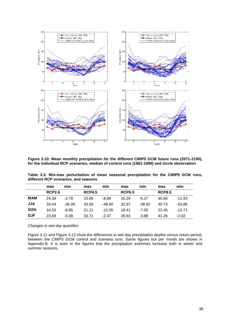
38

Figure 3.10: Mean monthly precipitation for the different CMIP5 GCM future runs (2071-2100), for the individual RCP scenarios, median of control runs (1961-1990) and Uccle observation

Table 3.3: Min-max perturbation of mean seasonal precipitation for the CMIP5 GCM runs, different RCP scenarios, and seasons

max min max min max min max min

RCP2.6

RCP4.5

RCP6.0

RCP8.5

MAM 24.38 -2.79 23.06 -8.86 16.29 -6.27 40.60 -11.93

JJA 33.44 -36.06 33.56 -48.60 32.97 -38.92 40.73 -53.86

SON 16.53 -8.85 21.21 -12.05 18.41 -7.05 22.45 -13.71

DJF 23.69 -0.38 33.71 -2.47 28.93 -3.88 41.26 -2.02

Changes in wet day quantiles

Figure 3.11 and Figure 3.12 show the differences in wet day precipitation depths versus return period, between the CMIP5 GCM control and scenario runs. Same figures but per month are shown in Appendix B. It is seen in the figures that the precipitation extremes increase both in winter and summer seasons.

39

Figure 3.11: Wet day precipitation intensities vs. return period: comparison of CMIP5 GCM control (1961-1990) with Uccle observation and scenario (2071-2100) runs with median of control runs, for all RCP scenarios and winter season

Figure 3.12: Wet day precipitation intensities vs. return period: comparison of control (1961-1990) with Uccle observation and scenario (2071-2100) runs with median of control runs, for all RCP scenarios and summer season

The projected change factors (relative changes) for the winter (DJF) and summer (JJA) seasons are shown in Figure 3.13. The daily relative changes factors were obtained for the rainfall quantiles that correspond to the highest 300 daily rainfall intensities in the 30-year runs (hence for return periods >0.1 year) and the high, mean and low scenario changes were identified. It can be seen that the range of change is wider for the summer season compared to that of the winter season. These factors also illustrate that the changes for the summer season increase for higher return periods, whereas the changes are approximately constant (independent of the return period) for the winter season.

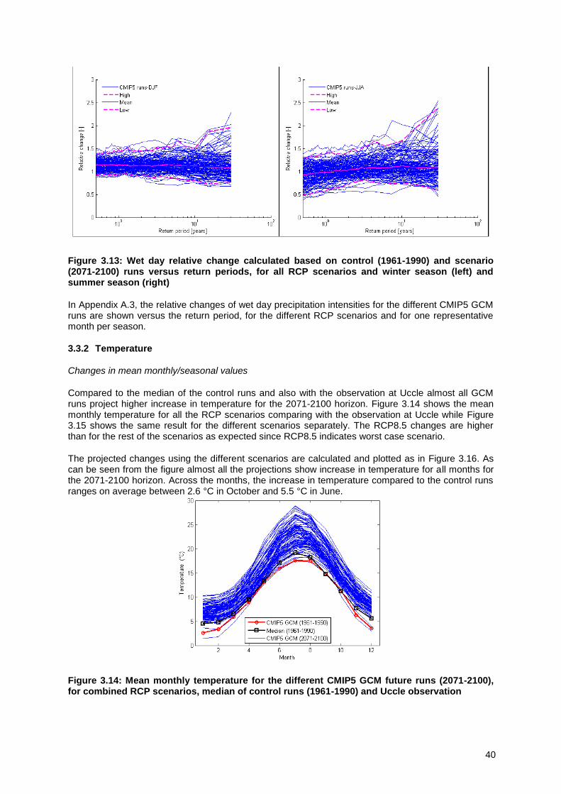
40

Figure 3.13: Wet day relative change calculated based on control (1961-1990) and scenario (2071-2100) runs versus return periods, for all RCP scenarios and winter season (left) and summer season (right)

In Appendix A.3, the relative changes of wet day precipitation intensities for the different CMIP5 GCM runs are shown versus the return period, for the different RCP scenarios and for one representative month per season.

3.3.2 Temperature

Changes in mean monthly/seasonal values

Compared to the median of the control runs and also with the observation at Uccle almost all GCM runs project higher increase in temperature for the 2071-2100 horizon. Figure 3.14 shows the mean monthly temperature for all the RCP scenarios comparing with the observation at Uccle while Figure 3.15 shows the same result for the different scenarios separately. The RCP8.5 changes are higher than for the rest of the scenarios as expected since RCP8.5 indicates worst case scenario.

The projected changes using the different scenarios are calculated and plotted as in Figure 3.16. As can be seen from the figure almost all the projections show increase in temperature for all months for the 2071-2100 horizon. Across the months, the increase in temperature compared to the control runs ranges on average between 2.6 °C in October and 5.5 °C in June.

Figure 3.14: Mean monthly temperature for the different CMIP5 GCM future runs (2071-2100), for combined RCP scenarios, median of control runs (1961-1990) and Uccle observation

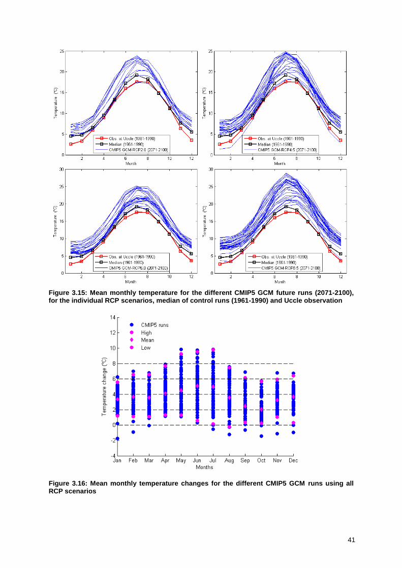
41

Figure 3.15: Mean monthly temperature for the different CMIP5 GCM future runs (2071-2100), for the individual RCP scenarios, median of control runs (1961-1990) and Uccle observation

Figure 3.16: Mean monthly temperature changes for the different CMIP5 GCM runs using all RCP scenarios

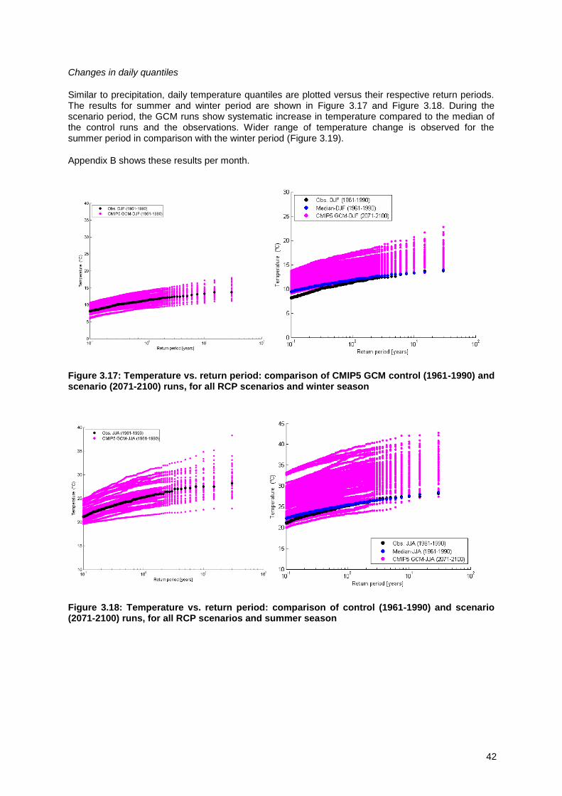
42

Changes in daily quantiles

Similar to precipitation, daily temperature quantiles are plotted versus their respective return periods. The results for summer and winter period are shown in Figure 3.17 and Figure 3.18. During the scenario period, the GCM runs show systematic increase in temperature compared to the median of the control runs and the observations. Wider range of temperature change is observed for the summer period in comparison with the winter period (Figure 3.19).

Appendix B shows these results per month.

Figure 3.17: Temperature vs. return period: comparison of CMIP5 GCM control (1961-1990) and scenario (2071-2100) runs, for all RCP scenarios and winter season

Figure 3.18: Temperature vs. return period: comparison of control (1961-1990) and scenario (2071-2100) runs, for all RCP scenarios and summer season

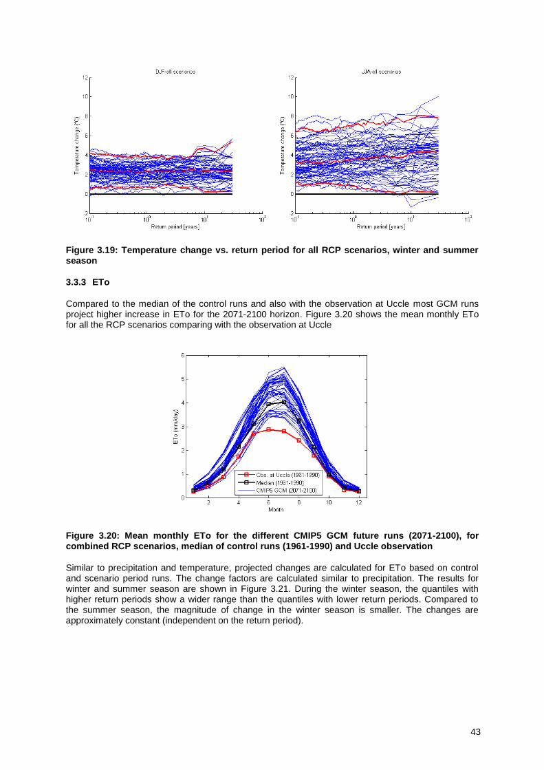
43

Figure 3.19: Temperature change vs. return period for all RCP scenarios, winter and summer season

3.3.3 ETo

Compared to the median of the control runs and also with the observation at Uccle most GCM runs project higher increase in ETo for the 2071-2100 horizon. Figure 3.20 shows the mean monthly ETo for all the RCP scenarios comparing with the observation at Uccle

Figure 3.20: Mean monthly ETo for the different CMIP5 GCM future runs (2071-2100), for combined RCP scenarios, median of control runs (1961-1990) and Uccle observation

Similar to precipitation and temperature, projected changes are calculated for ETo based on control and scenario period runs. The change factors are calculated similar to precipitation. The results for winter and summer season are shown in Figure 3.21. During the winter season, the quantiles with higher return periods show a wider range than the quantiles with lower return periods. Compared to the summer season, the magnitude of change in the winter season is smaller. The changes are approximately constant (independent on the return period).

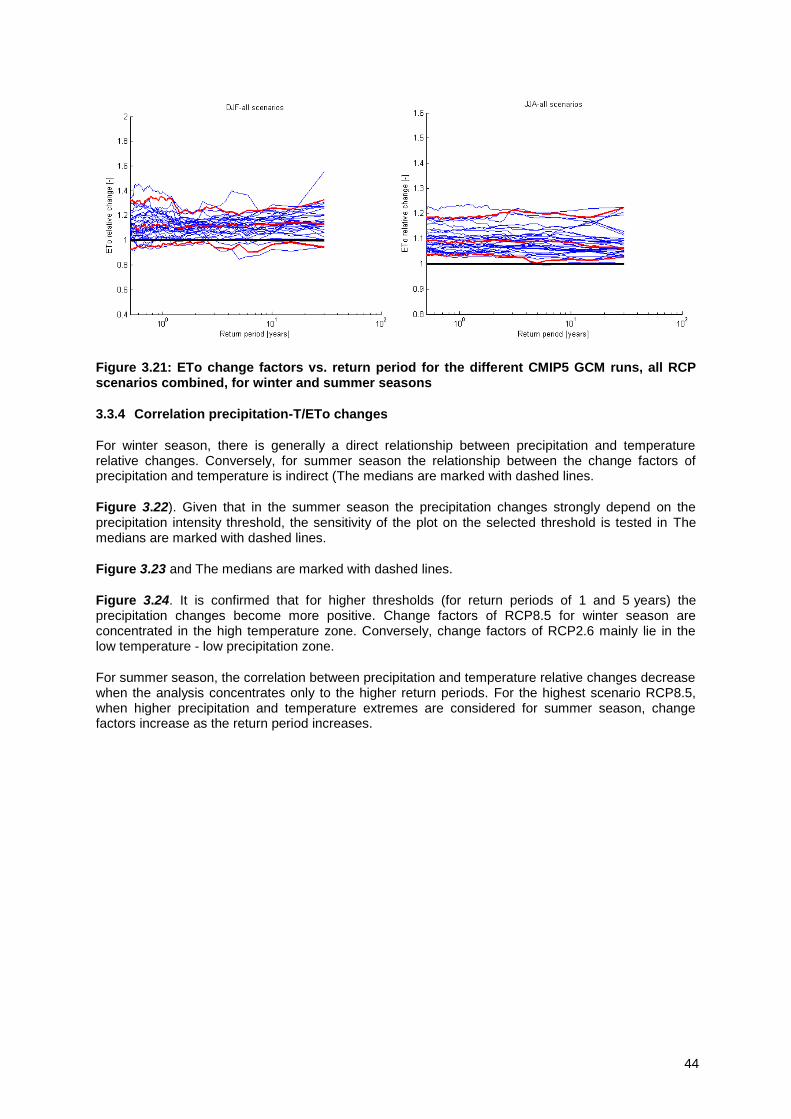
44

Figure 3.21: ETo change factors vs. return period for the different CMIP5 GCM runs, all RCP scenarios combined, for winter and summer seasons

3.3.4 Correlation precipitation-T/ETo changes

For winter season, there is generally a direct relationship between precipitation and temperature relative changes. Conversely, for summer season the relationship between the change factors of precipitation and temperature is indirect (The medians are marked with dashed lines.

Figure 3.22). Given that in the summer season the precipitation changes strongly depend on the precipitation intensity threshold, the sensitivity of the plot on the selected threshold is tested in The medians are marked with dashed lines.

Figure 3.23 and The medians are marked with dashed lines.

Figure 3.24. It is confirmed that for higher thresholds (for return periods of 1 and 5 years) the precipitation changes become more positive. Change factors of RCP8.5 for winter season are concentrated in the high temperature zone. Conversely, change factors of RCP2.6 mainly lie in the low temperature - low precipitation zone.

For summer season, the correlation between precipitation and temperature relative changes decrease when the analysis concentrates only to the higher return periods. For the highest scenario RCP8.5, when higher precipitation and temperature extremes are considered for summer season, change factors increase as the return period increases.

45

The medians are marked with dashed lines.

Figure 3.22: Inter-seasonal tracing of precipitation and temperature relative changes (averaged for return periods >0.1 year) for the different RCP scenarios

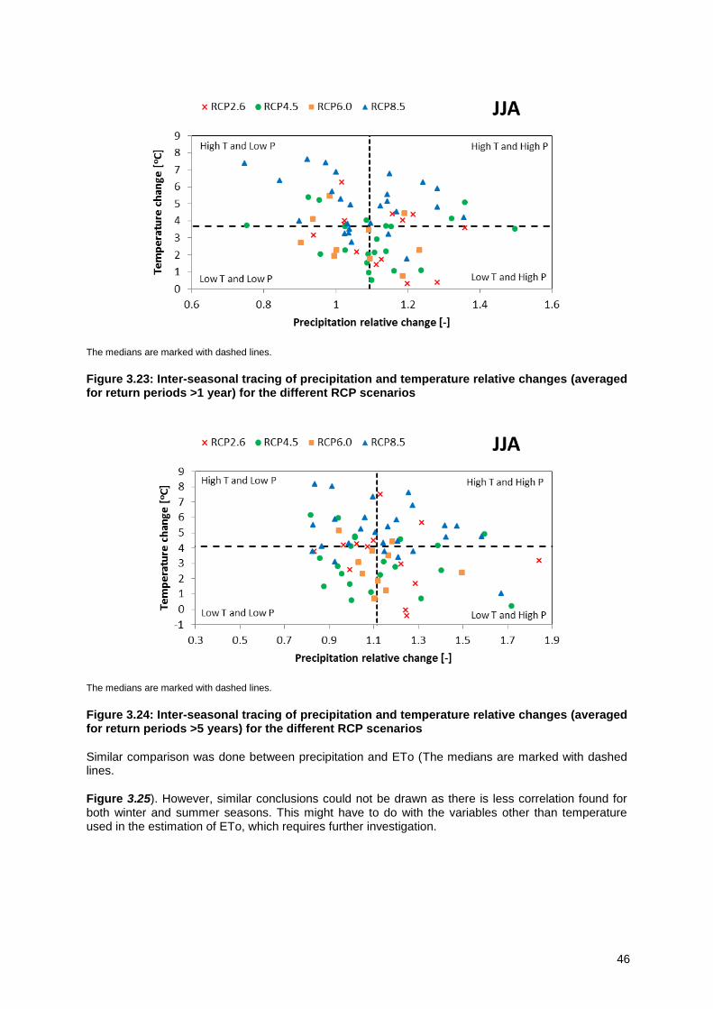
46


Figure 3.23: Inter-seasonal tracing of precipitation and temperature relative changes (averaged for return periods >1 year) for the different RCP scenarios


Figure 3.24: Inter-seasonal tracing of precipitation and temperature relative changes (averaged for return periods >5 years) for the different RCP scenarios

Similar comparison was done between precipitation and ETo (The medians are marked with dashed lines.

Figure 3.25). However, similar conclusions could not be drawn as there is less correlation found for both winter and summer seasons. This might have to do with the variables other than temperature used in the estimation of ETo, which requires further investigation.

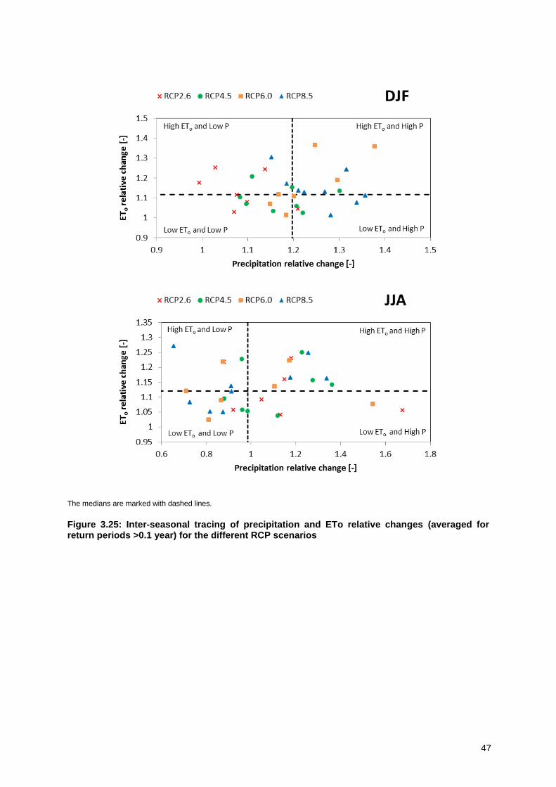
47


Figure 3.25: Inter-seasonal tracing of precipitation and ETo relative changes (averaged for return periods >0.1 year) for the different RCP scenarios

48

3.3.5 Conclusions

The main findings from this analysis of the climatic changes in precipitation, temperature and ETo are:

Mean summer precipitation consistently decreases for most of the runs.

Number of wet days are projected to decrease in summer season and increase in winter season.

Precipitation extremes are projected to increase during winter season for most of the runs at all return period levels.

On average precipitation extremes are projected to decrease during summer season for the lower precipitation intensities and the changes increase (and become positive for many runs) for the higher return periods.

Temperature is projected to increase for all seasons; on average by 3 °C for winter season and 4.5 °C for summer season. The increasing signal in summer is higher than that of the winter.

Similarly, evapotranspiration is projected to increase for summer season higher than winter season.

The decrease in precipitation frequency and intensity as well as the increase in temperature for summer season shows that much drier conditions are expected for this season.

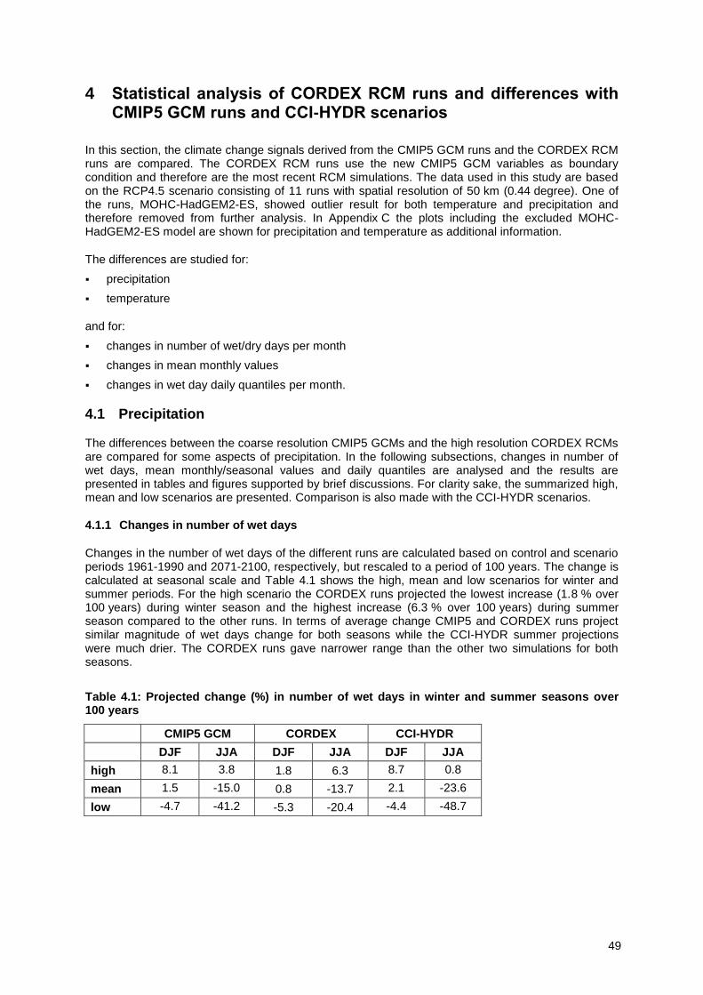
49

4 Statistical analysis of CORDEX RCM runs and differences with CMIP5 GCM runs and CCI-HYDR scenarios

In this section, the climate change signals derived from the CMIP5 GCM runs and the CORDEX RCM runs are compared. The CORDEX RCM runs use the new CMIP5 GCM variables as boundary condition and therefore are the most recent RCM simulations. The data used in this study are based on the RCP4.5 scenario consisting of 11 runs with spatial resolution of 50 km (0.44 degree). One of the runs, MOHC-HadGEM2-ES, showed outlier result for both temperature and precipitation and therefore removed from further analysis. In Appendix C the plots including the excluded MOHC-HadGEM2-ES model are shown for precipitation and temperature as additional information.

The differences are studied for:

precipitation

temperature

and for:

changes in number of wet/dry days per month

changes in mean monthly values

changes in wet day daily quantiles per month.

4.1 Precipitation

The differences between the coarse resolution CMIP5 GCMs and the high resolution CORDEX RCMs are compared for some aspects of precipitation. In the following subsections, changes in number of wet days, mean monthly/seasonal values and daily quantiles are analysed and the results are presented in tables and figures supported by brief discussions. For clarity sake, the summarized high, mean and low scenarios are presented. Comparison is also made with the CCI-HYDR scenarios.

4.1.1 Changes in number of wet days

Changes in the number of wet days of the different runs are calculated based on control and scenario periods 1961-1990 and 2071-2100, respectively, but rescaled to a period of 100 years. The change is calculated at seasonal scale and Table 4.1 shows the high, mean and low scenarios for winter and summer periods. For the high scenario the CORDEX runs projected the lowest increase (1.8 % over 100 years) during winter season and the highest increase (6.3 % over 100 years) during summer season compared to the other runs. In terms of average change CMIP5 and CORDEX runs project similar magnitude of wet days change for both seasons while the CCI-HYDR summer projections were much drier. The CORDEX runs gave narrower range than the other two simulations for both seasons.

Table 4.1: Projected change (%) in number of wet days in winter and summer seasons over 100 years

CMIP5 GCM CORDEX CCI-HYDR

DJF JJA DJF JJA DJF JJA

high 8.1 3.8 1.8 6.3 8.7 0.8

mean 1.5 -15.0 0.8 -13.7 2.1 -23.6

low -4.7 -41.2 -5.3 -20.4 -4.4 -48.7

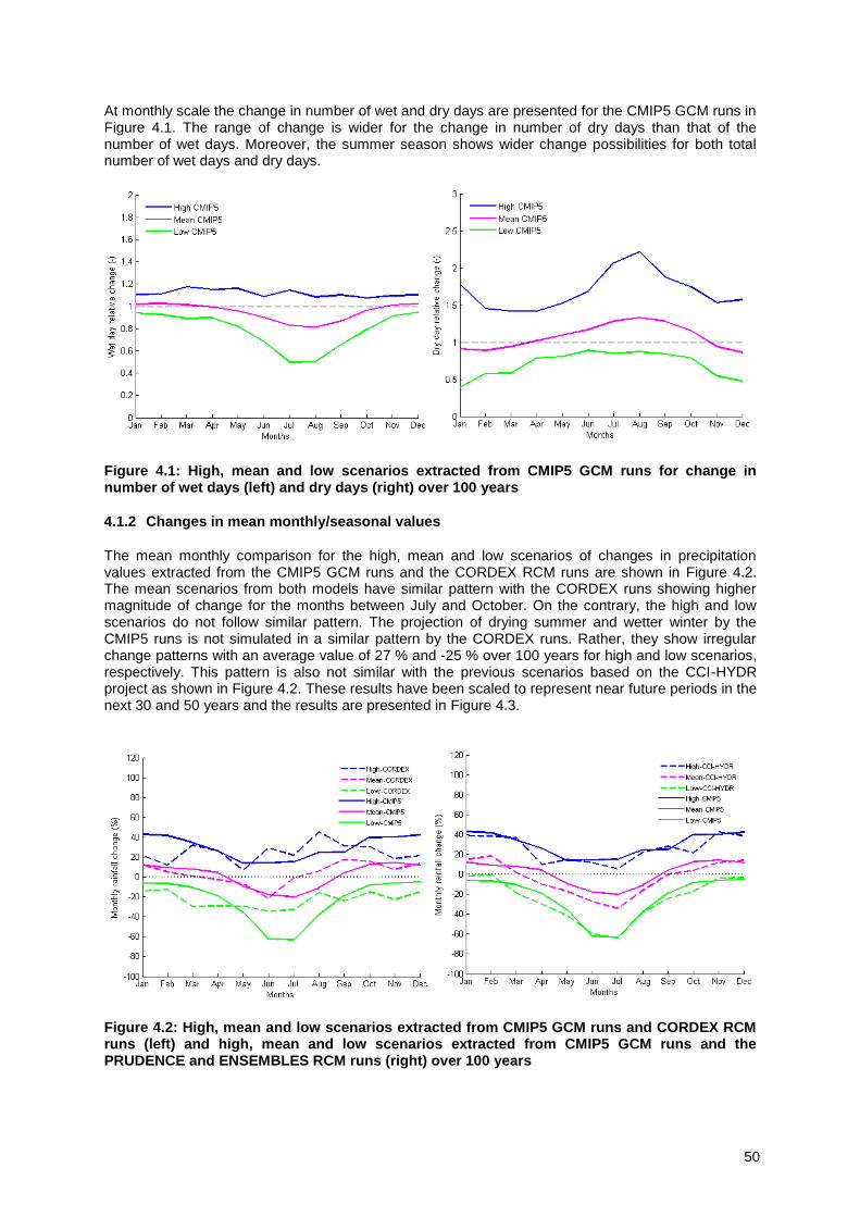
50

At monthly scale the change in number of wet and dry days are presented for the CMIP5 GCM runs in Figure 4.1. The range of change is wider for the change in number of dry days than that of the number of wet days. Moreover, the summer season shows wider change possibilities for both total number of wet days and dry days.

Figure 4.1: High, mean and low scenarios extracted from CMIP5 GCM runs for change in number of wet days (left) and dry days (right) over 100 years

4.1.2 Changes in mean monthly/seasonal values

The mean monthly comparison for the high, mean and low scenarios of changes in precipitation values extracted from the CMIP5 GCM runs and the CORDEX RCM runs are shown in Figure 4.2. The mean scenarios from both models have similar pattern with the CORDEX runs showing higher magnitude of change for the months between July and October. On the contrary, the high and low scenarios do not follow similar pattern. The projection of drying summer and wetter winter by the CMIP5 runs is not simulated in a similar pattern by the CORDEX runs. Rather, they show irregular change patterns with an average value of 27 % and -25 % over 100 years for high and low scenarios, respectively. This pattern is also not similar with the previous scenarios based on the CCI-HYDR project as shown in Figure 4.2. These results have been scaled to represent near future periods in the next 30 and 50 years and the results are presented in Figure 4.3.

Figure 4.2: High, mean and low scenarios extracted from CMIP5 GCM runs and CORDEX RCM runs (left) and high, mean and low scenarios extracted from CMIP5 GCM runs and the PRUDENCE and ENSEMBLES RCM runs (right) over 100 years

51

Figure 4.3: High, mean and low scenarios extracted from CMIP5 GCM runs and the PRUDENCE and ENSEMBLES RCM runs over 30 years (left) and 50 years (right)

The mean seasonal comparison was conducted for winter and summer seasons. The results are presented in Table 4.2. From the table it can be seen that the projected changes by CORDEX for both periods are lower than the CMIP5 and CCI-HYDR scenarios, especially for the high scenario. This can be attributed to the fact that the CORDEX runs are based on the RCP4.5 scenarios which are in the lower side of the full range of CMIP5 GCM runs. The difference in the mean scenario is in the order of 2 % over 100 years between the CMIP5 and CORDEX runs, which is not that large and can lead to the conclusion that both high and low resolution models gave comparable results. In addition, from the mean scenarios of the three runs one can see the drier summer and wetter winter projections that is consistent. The CORDEX runs projected much drier winter using the low scenario unlike the other runs that showed almost no change. Conversely, the summer period drying magnitude (-24 % over 100 years) is about half of as the projections by the other runs (-52 %).

Table 4.2: Projected change (%) in mean seasonal values in winter and summer seasons over 100 years



high 37.7 18.0 14.0 7.1 30.5 9.5

mean 11.5 -14.7 9.2 -16.3 14.9 -26.5

low -1.2 -52.0 -16.2 -23.8 2.0 -52.7

4.1.3 Changes in wet day quantiles

Changes in daily quantiles are calculated for all empirical return periods and presented as change factors, which are the ratios between scenario and control period values. This is done at seasonal time scales and the results for winter and summer seasons are shown in Figure 4.4. For both seasons CORDEX runs are on the lower side when comparing their high scenario with that of the CMIP5 runs, while the mean and low scenarios are similar. Again this can be partially attributed to the CORDEX runs being solely based on RCP4.5.

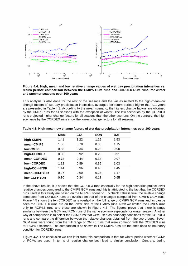
52

Figure 4.4: High, mean and low relative change values of wet day precipitation intensities vs. return period: comparison between the CMIP5 GCM runs and CORDEX RCM runs, for winter and summer seasons over 100 years

This analysis is also done for the rest of the seasons and the values related to the high-mean-low change factors of wet day precipitation intensities, averaged for return periods higher than 0.1 years are presented in Table 4.3. According to the mean scenario, the highest change factors are obtained by the CMIP5 runs for all seasons with the exception of winter. The low scenarios by the CORDEX runs projected higher change factors for all seasons than the other two runs. On the contrary, the high scenarios by the CORDEX runs show the lowest change factors for all seasons.

Table 4.3: High-mean-low change factors of wet day precipitation intensities over 100 years

MAM JJA SON DJF

high-CMIP5 1.41 1.22 1.25 1.53

mean-CMIP5 1.06 0.78 0.35 1.15

low-CMIP5 0.88 0.34 0.23 0.90

high-CORDEX 0.80 0.92 0.20 0.91

mean-CORDEX 0.78 0.44 0.34 0.97

low- CORDEX 1.12 0.89 0.35 1.03

high-CCI-HYDR 1.14 0.96 0.43 1.45

mean-CCI-HYDR 0.97 0.60 0.25 1.17

low-CCI-HYDR 0.80 0.34 0.18 0.95

In the above results, it is shown that the CORDEX runs especially for the high scenarios project lower relative changes compared to the CMIP5 GCM runs and this is attributed to the fact that the CORDEX runs used in this study are based on the RCP4.5 scenario. To check if this is true, the relative change computed from CORDEX runs are overlaid on that of the changes computed from CMIP5 GCM runs. Figure 4.5 shows the ten CORDEX runs overlaid on the full range of CMIP5 GCM runs and as can be seen the CORDEX runs are on the lower side of the CMIP5 runs. Next we limited the CMIP5 runs only to RCP4.5 runs and these are shown in Figure 4.6. The figures prove that there is range similarity between the GCM and RCM runs of the same scenario especially for winter season. Another way of comparison is to select the GCM runs that were used as boundary conditions for the CORDEX runs and compare the difference between the relative changes obtained from the two groups. Seven GCM runs were found from the full range of CMIP5 runs that were common with the CORDEX runs for RCP4.5 scenario. The comparison is as shown in The CMIP5 runs are the ones used as boundary condition for CORDEX runs.

Figure 4.7. The conclusion we can infer from this comparison is that for winter period whether GCMs or RCMs are used, in terms of relative change both lead to similar conclusion. Contrary, during

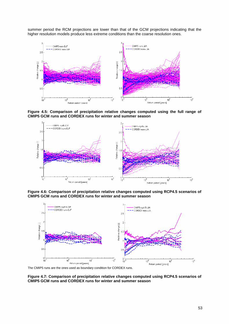
53

summer period the RCM projections are lower than that of the GCM projections indicating that the higher resolution models produce less extreme conditions than the coarse resolution ones.

Figure 4.5: Comparison of precipitation relative changes computed using the full range of CMIP5 GCM runs and CORDEX runs for winter and summer season

Figure 4.6: Comparison of precipitation relative changes computed using RCP4.5 scenarios of CMIP5 GCM runs and CORDEX runs for winter and summer season

The CMIP5 runs are the ones used as boundary condition for CORDEX runs.

Figure 4.7: Comparison of precipitation relative changes computed using RCP4.5 scenarios of CMIP5 GCM runs and CORDEX runs for winter and summer season

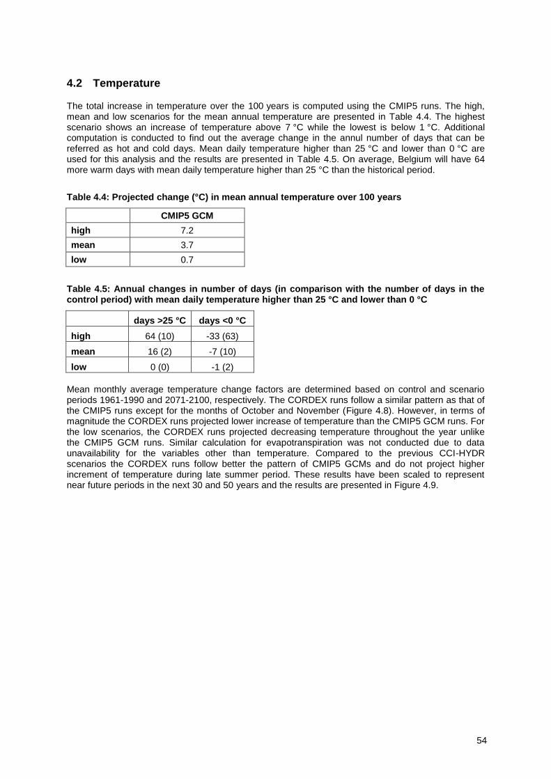
54

4.2 Temperature

The total increase in temperature over the 100 years is computed using the CMIP5 runs. The high, mean and low scenarios for the mean annual temperature are presented in Table 4.4. The highest scenario shows an increase of temperature above 7 °C while the lowest is below 1 °C. Additional computation is conducted to find out the average change in the annul number of days that can be referred as hot and cold days. Mean daily temperature higher than 25 °C and lower than 0 °C are used for this analysis and the results are presented in Table 4.5. On average, Belgium will have 64 more warm days with mean daily temperature higher than 25 °C than the historical period.

Table 4.4: Projected change (°C) in mean annual temperature over 100 years

CMIP5 GCM

high 7.2

mean 3.7

low 0.7

Table 4.5: Annual changes in number of days (in comparison with the number of days in the control period) with mean daily temperature higher than 25 °C and lower than 0 °C

days >25 °C days <0 °C

high 64 (10) -33 (63)

mean 16 (2) -7 (10)

low 0 (0) -1 (2)

Mean monthly average temperature change factors are determined based on control and scenario periods 1961-1990 and 2071-2100, respectively. The CORDEX runs follow a similar pattern as that of the CMIP5 runs except for the months of October and November (Figure 4.8). However, in terms of magnitude the CORDEX runs projected lower increase of temperature than the CMIP5 GCM runs. For the low scenarios, the CORDEX runs projected decreasing temperature throughout the year unlike the CMIP5 GCM runs. Similar calculation for evapotranspiration was not conducted due to data unavailability for the variables other than temperature. Compared to the previous CCI-HYDR scenarios the CORDEX runs follow better the pattern of CMIP5 GCMs and do not project higher increment of temperature during late summer period. These results have been scaled to represent near future periods in the next 30 and 50 years and the results are presented in Figure 4.9.

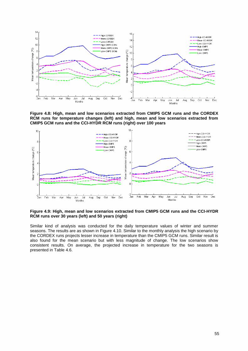
55

Figure 4.8: High, mean and low scenarios extracted from CMIP5 GCM runs and the CORDEX RCM runs for temperature changes (left) and high, mean and low scenarios extracted from CMIP5 GCM runs and the CCI-HYDR RCM runs (right) over 100 years

Figure 4.9: High, mean and low scenarios extracted from CMIP5 GCM runs and the CCI-HYDR RCM runs over 30 years (left) and 50 years (right)

Similar kind of analysis was conducted for the daily temperature values of winter and summer seasons. The results are as shown in Figure 4.10. Similar to the monthly analysis the high scenario by the CORDEX runs projects lesser increase in temperature than the CMIP5 GCM runs. Similar result is also found for the mean scenario but with less magnitude of change. The low scenarios show consistent results. On average, the projected increase in temperature for the two seasons is presented in Table 4.6.

56

Figure 4.10: High, mean and low relative change values of daily temperature vs. return period: comparison between the CMIP5 GCM runs and CORDEX RCM runs, for winter and summer seasons over 100 years

Table 4.6: Projected temperature change (°C) in mean seasonal values in winter and summer seasons over 100 years



high 6.2 8.9 2.4 3.4 3.9 6.5

mean 3.6 4.5 1.0 1.0 2.6 4.0

low 0.9 0.2 -0.4 -1.1 1.1 2.1

If the GCM runs are limited to the models that were used as boundary conditions for CORDEX runs and compared with the temperature changes obtained from CORDEX runs, the results obtained are as shown in The CMIP5 runs are the ones used as boundary condition for CORDEX runs.

Figure 4.11. Similar to precipitation one can see that the magnitude of the high scenarios is lower compared to Figure 4.10. This is again attributed to the fact that the CORDEX runs analysed in this study used the RCP4.5 scenarios that are on the lower side of the full CMIP5 runs. Compared to winter season, the summer season shows wider ranges of projections.

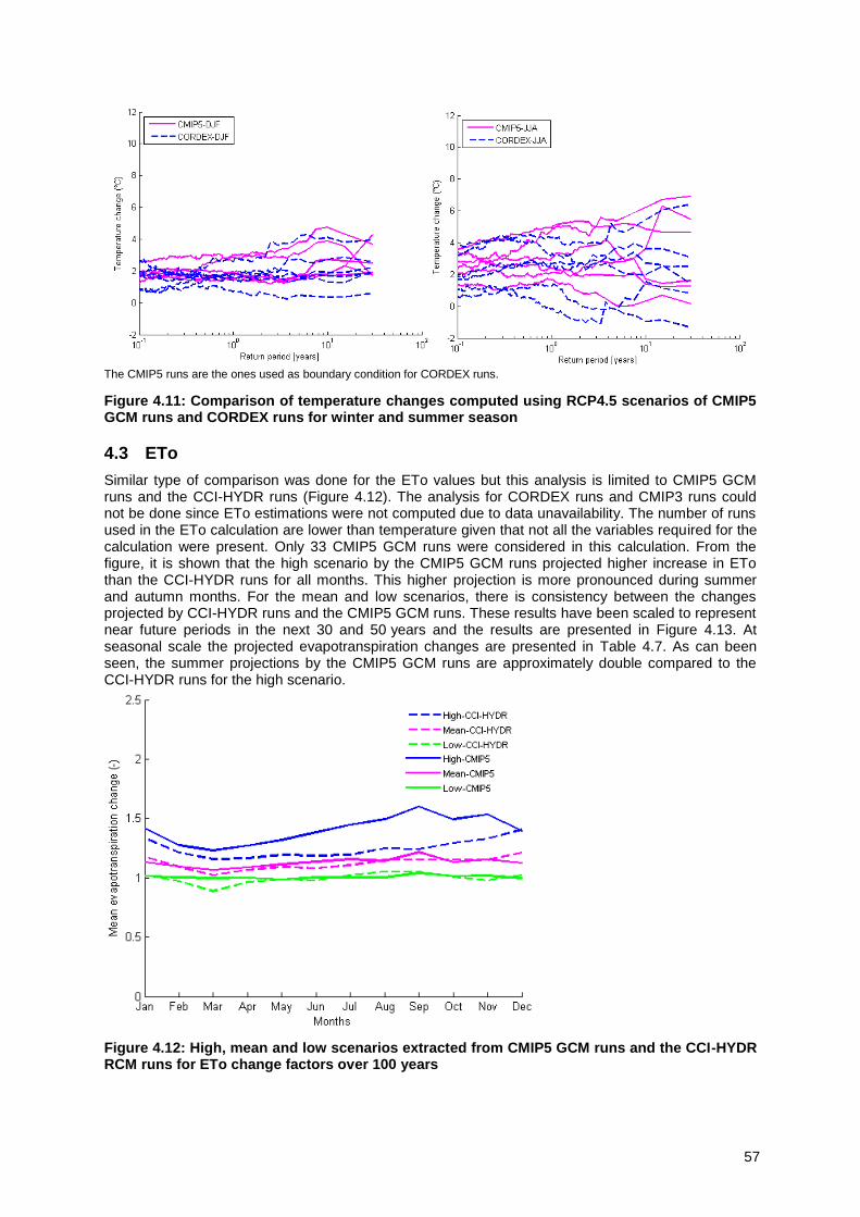
57

The CMIP5 runs are the ones used as boundary condition for CORDEX runs.

Figure 4.11: Comparison of temperature changes computed using RCP4.5 scenarios of CMIP5 GCM runs and CORDEX runs for winter and summer season

4.3 ETo

Similar type of comparison was done for the ETo values but this analysis is limited to CMIP5 GCM runs and the CCI-HYDR runs (Figure 4.12). The analysis for CORDEX runs and CMIP3 runs could not be done since ETo estimations were not computed due to data unavailability. The number of runs used in the ETo calculation are lower than temperature given that not all the variables required for the calculation were present. Only 33 CMIP5 GCM runs were considered in this calculation. From the figure, it is shown that the high scenario by the CMIP5 GCM runs projected higher increase in ETo than the CCI-HYDR runs for all months. This higher projection is more pronounced during summer and autumn months. For the mean and low scenarios, there is consistency between the changes projected by CCI-HYDR runs and the CMIP5 GCM runs. These results have been scaled to represent near future periods in the next 30 and 50 years and the results are presented in Figure 4.13. At seasonal scale the projected evapotranspiration changes are presented in Table 4.7. As can been seen, the summer projections by the CMIP5 GCM runs are approximately double compared to the CCI-HYDR runs for the high scenario.

Figure 4.12: High, mean and low scenarios extracted from CMIP5 GCM runs and the CCI-HYDR RCM runs for ETo change factors over 100 years

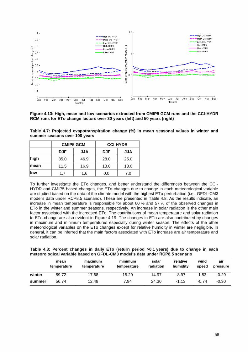
58

Figure 4.13: High, mean and low scenarios extracted from CMIP5 GCM runs and the CCI-HYDR RCM runs for ETo change factors over 30 years (left) and 50 years (right)

Table 4.7: Projected evapotranspiration change (%) in mean seasonal values in winter and summer seasons over 100 years

CMIP5 GCM CCI-HYDR

DJF JJA DJF JJA

high 35.0 46.9 28.0 25.0

mean 11.5 16.9 13.0 13.0

low 1.7 1.6 0.0 7.0

To further investigate the ETo changes, and better understand the differences between the CCI-HYDR and CMIP5 based changes, the ETo changes due to change in each meteorological variable are studied based on the data of the climate model with the highest ETo perturbation (i.e., GFDL-CM3 model’s data under RCP8.5 scenario). These are presented in Table 4.8. As the results indicate, an increase in mean temperature is responsible for about 60 % and 57 % of the observed changes in ETo in the winter and summer seasons, respectively. An increase in solar radiation is the other main factor associated with the increased ETo. The contributions of mean temperature and solar radiation to ETo change are also evident in Figure 4.19. The changes in ETo are also contributed by changes in maximum and minimum temperatures especially during winter season. The effects of the other meteorological variables on the ETo changes except for relative humidity in winter are negligible. In general, it can be inferred that the main factors associated with ETo increase are air temperature and solar radiation.

Table 4.8: Percent changes in daily ETo (return period >0.1 years) due to change in each meteorological variable based on GFDL-CM3 model’s data under RCP8.5 scenario

mean

temperature

maximum

temperature

minimum

temperature

solar

radiation

relative

humidity

wind

speed

air

pressure

winter 59.72 17.68 15.29 14.97 -8.97 1.53 -0.29

summer 56.74 12.48 7.94 24.30 -1.13 -0.74 -0.30

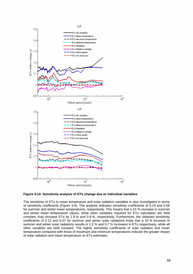
59

Figure 4.14: Sensitivity analysis of ETo change due to individual variables

The sensitivity of ETo to mean temperature and solar radiation variables is also investigated in terms of sensitivity coefficients (Figure 4.9). The analysis indicates sensitivity coefficients of 0.19 and 0.09 for summer and winter mean temperatures, respectively. This means that a 10 % increase in summer and winter mean temperature values, while other variables required for ETo calculation are held constant, may increase ETo by 1.9 % and 0.9 %, respectively. Furthermore, the obtained sensitivity coefficients of 0.12 and 0.07 for summer and winter solar radiations imply that a 10 % increase in summer and winter solar radiations results in 1.2 % and 0.7 % increases in ETo respectively, while all other variables are held constant. The higher sensitivity coefficients of solar radiation and mean temperature compared with those of maximum and minimum temperatures indicate the greater impact of solar radiation and mean temperature on ETo estimates.

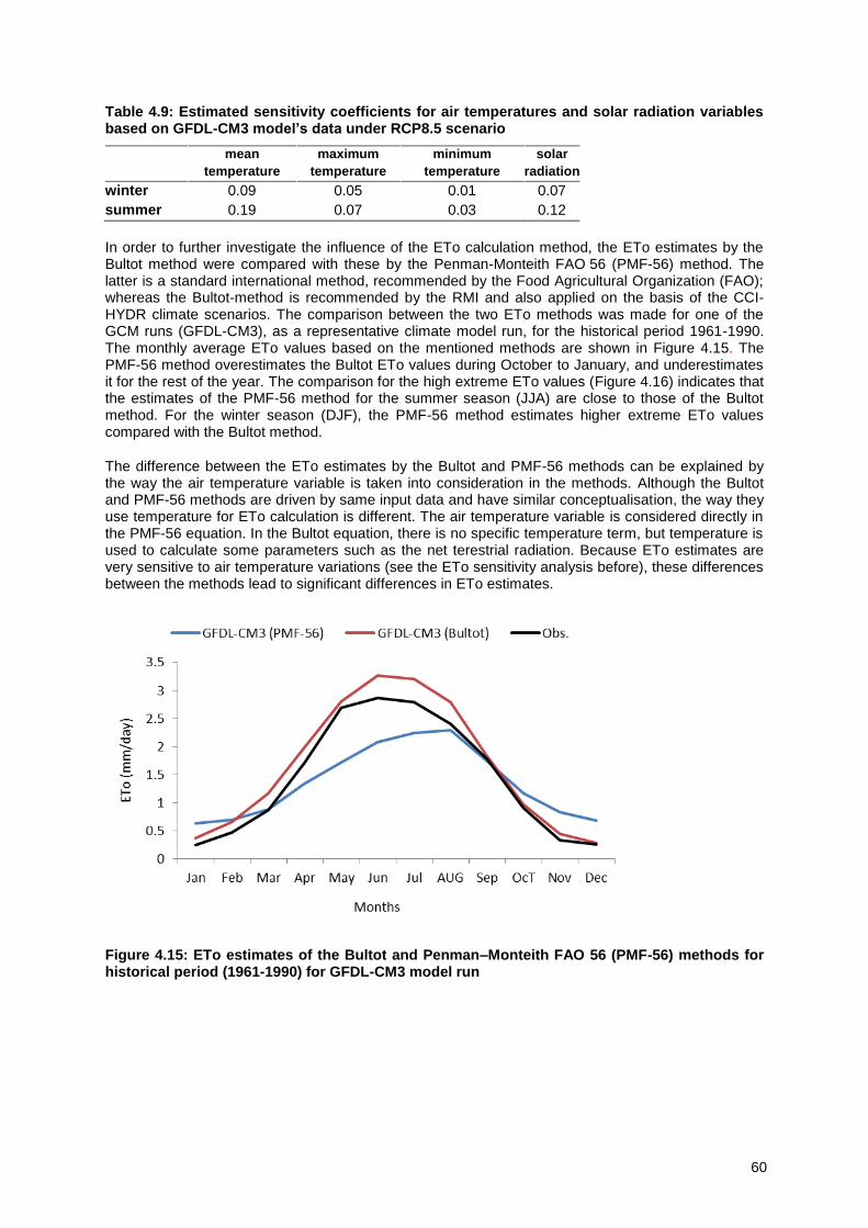
60

Table 4.9: Estimated sensitivity coefficients for air temperatures and solar radiation variables based on GFDL-CM3 model’s data under RCP8.5 scenario

mean

temperature

maximum

temperature

minimum

temperature

solar

radiation

winter 0.09 0.05 0.01 0.07

summer 0.19 0.07 0.03 0.12

In order to further investigate the influence of the ETo calculation method, the ETo estimates by the Bultot method were compared with these by the Penman-Monteith FAO 56 (PMF-56) method. The latter is a standard international method, recommended by the Food Agricultural Organization (FAO); whereas the Bultot-method is recommended by the RMI and also applied on the basis of the CCI-HYDR climate scenarios. The comparison between the two ETo methods was made for one of the GCM runs (GFDL-CM3), as a representative climate model run, for the historical period 1961-1990. The monthly average ETo values based on the mentioned methods are shown in Figure 4.15. The PMF-56 method overestimates the Bultot ETo values during October to January, and underestimates it for the rest of the year. The comparison for the high extreme ETo values (Figure 4.16) indicates that the estimates of the PMF-56 method for the summer season (JJA) are close to those of the Bultot method. For the winter season (DJF), the PMF-56 method estimates higher extreme ETo values compared with the Bultot method.

The difference between the ETo estimates by the Bultot and PMF-56 methods can be explained by the way the air temperature variable is taken into consideration in the methods. Although the Bultot and PMF-56 methods are driven by same input data and have similar conceptualisation, the way they use temperature for ETo calculation is different. The air temperature variable is considered directly in the PMF-56 equation. In the Bultot equation, there is no specific temperature term, but temperature is used to calculate some parameters such as the net terestrial radiation. Because ETo estimates are very sensitive to air temperature variations (see the ETo sensitivity analysis before), these differences between the methods lead to significant differences in ETo estimates.

Figure 4.15: ETo estimates of the Bultot and Penman–Monteith FAO 56 (PMF-56) methods for historical period (1961-1990) for GFDL-CM3 model run

61

Figure 4.16: ETo vs. return period: comparison of the Bultot and Penman–Monteith FAO 56 (PMF-56) methods for historical period (1961-1990), for winter and summer season

Because there exists no direct observations of ETo, hence no reference data to decide on the accuracy of both methods, this study follows the recommended method by the RMI, which was calibrated specifically for Belgian conditions. At the same time, the sensitivity analysis conducted here shows the need for more detailed investigations on ETo estimation for Belgium/Flanders. Such investigation goes beyond the scope of the present study.

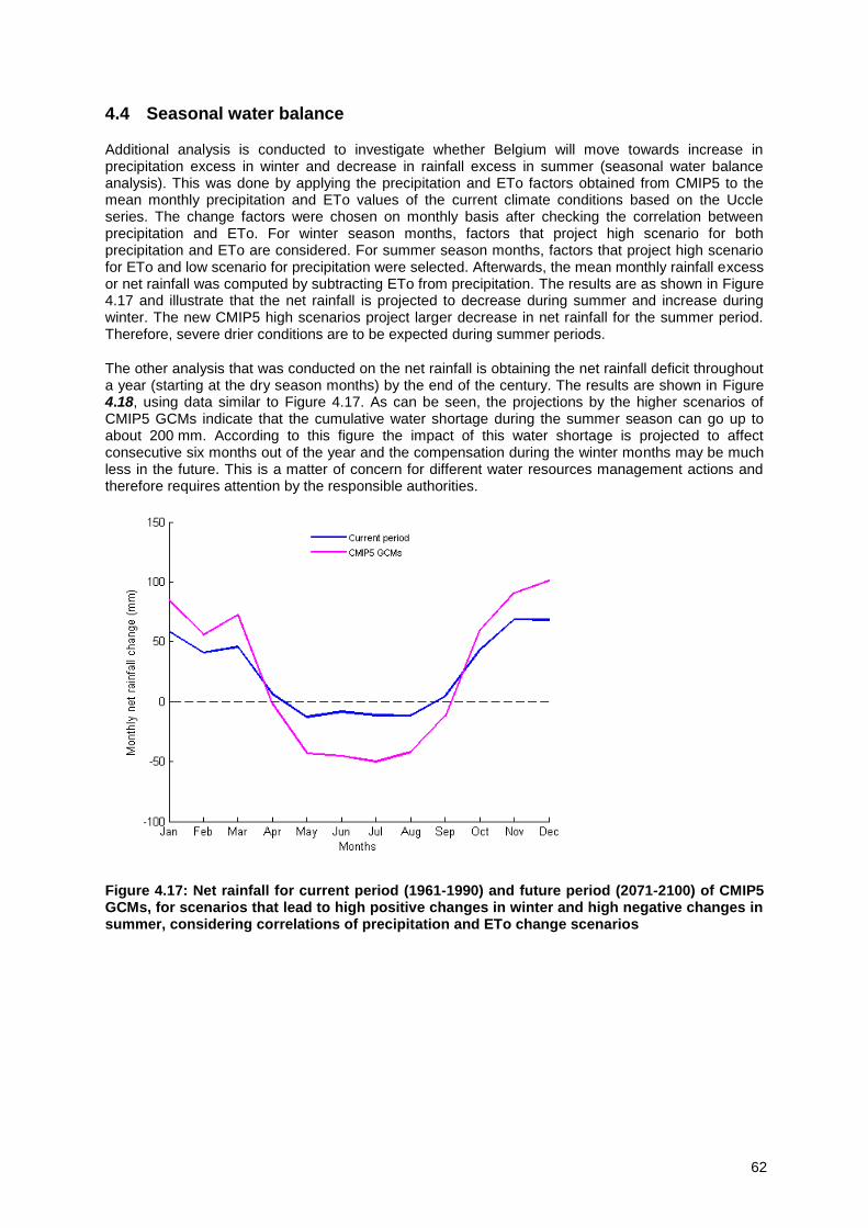
62

4.4 Seasonal water balance

Additional analysis is conducted to investigate whether Belgium will move towards increase in precipitation excess in winter and decrease in rainfall excess in summer (seasonal water balance analysis). This was done by applying the precipitation and ETo factors obtained from CMIP5 to the mean monthly precipitation and ETo values of the current climate conditions based on the Uccle series. The change factors were chosen on monthly basis after checking the correlation between precipitation and ETo. For winter season months, factors that project high scenario for both precipitation and ETo are considered. For summer season months, factors that project high scenario for ETo and low scenario for precipitation were selected. Afterwards, the mean monthly rainfall excess or net rainfall was computed by subtracting ETo from precipitation. The results are as shown in Figure 4.17 and illustrate that the net rainfall is projected to decrease during summer and increase during winter. The new CMIP5 high scenarios project larger decrease in net rainfall for the summer period. Therefore, severe drier conditions are to be expected during summer periods.

The other analysis that was conducted on the net rainfall is obtaining the net rainfall deficit throughout a year (starting at the dry season months) by the end of the century. The results are shown in Figure 4.18, using data similar to Figure 4.17. As can be seen, the projections by the higher scenarios of CMIP5 GCMs indicate that the cumulative water shortage during the summer season can go up to about 200 mm. According to this figure the impact of this water shortage is projected to affect consecutive six months out of the year and the compensation during the winter months may be much less in the future. This is a matter of concern for different water resources management actions and therefore requires attention by the responsible authorities.

Figure 4.17: Net rainfall for current period (1961-1990) and future period (2071-2100) of CMIP5 GCMs, for scenarios that lead to high positive changes in winter and high negative changes in summer, considering correlations of precipitation and ETo change scenarios

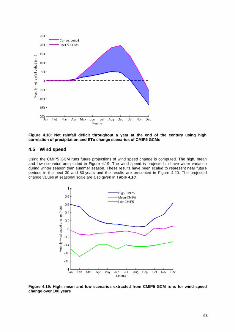
63

Figure 4.18: Net rainfall deficit throughout a year at the end of the century using high correlation of precipitation and ETo change scenarios of CMIP5 GCMs

4.5 Wind speed

Using the CMIP5 GCM runs future projections of wind speed change is computed. The high, mean and low scenarios are plotted in Figure 4.19. The wind speed is projected to have wider variation during winter season than summer season. These results have been scaled to represent near future periods in the next 30 and 50 years and the results are presented in Figure 4.20. The projected change values at seasonal scale are also given in Table 4.10.

Figure 4.19: High, mean and low scenarios extracted from CMIP5 GCM runs for wind speed change over 100 years

64

Figure 4.20: High, mean and low scenarios extracted from CMIP5 GCM runs for wind speed change over 30 years (left) and 50 years (right)

Table 4.10: Projected wind speed change (%) in mean seasonal values in winter and summer seasons over 100 years

CMIP5 GCM

DJF JJA

high 11 6

mean -1 -3

low -28 -16

4.6 Correlation between precipitation and temperature changes

The correlation between precipitation and temperature by CORDEX runs show that there is a positive correlation during winter and a negative correlation during summer. This analysis was done for quantiles greater than return period of 0.1 year and 1 year (red crosses in The medians are marked with dashed lines.


Figure 4.22, respectively). For both return periods the pattern is similar with quantiles of greater than 0.1 year showing clearer relationship. In the same plots, the GCM runs used as boundary condition for the CORDEX RCMs are plotted (green triangles in The medians are marked with dashed lines.


Figure 4.22). The relationship between the GCM runs of precipitation and temperature follows the CORDEX runs correlation for summer season than winter season.

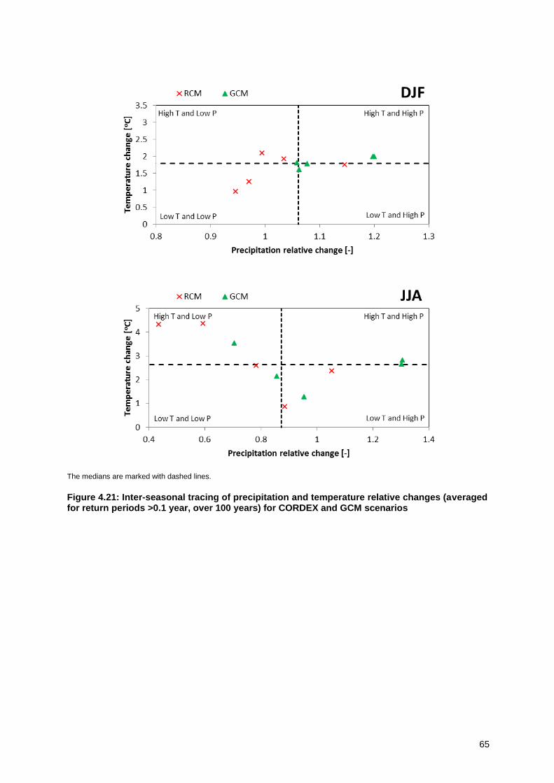
65


Figure 4.21: Inter-seasonal tracing of precipitation and temperature relative changes (averaged for return periods >0.1 year, over 100 years) for CORDEX and GCM scenarios

66


Figure 4.22: Inter-seasonal tracing of precipitation and temperature relative changes (averaged for return periods >1 year, over 100 years) for CORDEX and GCM scenarios

4.7 Conclusions

The main findings from this analysis of comparing CMIP5 GCMs, CCI-HYDR and CORDEX RCMs scenarios are:

The CORDEX runs do not follow the same pattern as that of the other runs for mean monthly precipitation changes especially for high and low scenarios.

The high scenarios of CORDEX results for temperature are projected to be lower in magnitude than the CMIP5 runs.

The fact that CORDEX runs are based on the RCP4.5 scenario has an influence on the results (especially on the high scenarios).

The correlation between the change in precipitation and temperature is as positive for winter and negative for summer. This is consistent with what is expected in these seasons.

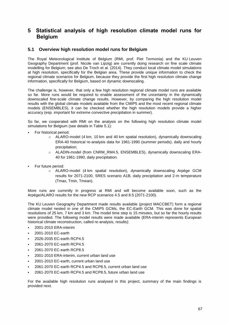
67

5 Statistical analysis of high resolution climate model runs for Belgium

5.1 Overview high resolution model runs for Belgium

The Royal Meteorological Institute of Belgium (RMI, prof. Piet Termonia) and the KU Leuven Geography Department (prof. Nicole van Lipzig) are currently doing research on fine scale climate modelling for Belgium; see also De Troch et al. (2014). They conduct local climate model simulations at high resolution, specifically for the Belgian area. These provide unique information to check the regional climate scenarios for Belgium, because they provide the first high resolution climate change information, specifically for Belgium, based on dynamic downscaling.

The challenge is, however, that only a few high resolution regional climate model runs are available so far. More runs would be required to enable assessment of the uncertainty in the dynamically downscaled fine-scale climate change results. However, by comparing the high resolution model results with the global climate models available from the CMIP5 and the most recent regional climate models (ENSEMBLES), it can be checked whether the high resolution models provide a higher accuracy (esp. important for extreme convective precipitation in summer).

So far, we cooperated with RMI on the analysis on the following high resolution climate model simulations for Belgium (see details in Table 5.1):

For historical period: o ALARO-model (4 km, 10 km and 40 km spatial resolution), dynamically downscaling

ERA-40 historical re-analysis data for 1961-1990 (summer periods), daily and hourly

precipitation;

o ALADIN-model (from CNRM_RM4.5, ENSEMBLES), dynamically downscaling ERA-

40 for 1961-1990, daily precipitation.

For future period: o ALARO-model (4 km spatial resolution), dynamically downscaling Arpège GCM

results for 2071-2100, SRES scenario A1B, daily precipitation and 2-m temperature

(Tmax, Tmin, Tmean).

More runs are currently in progress at RMI and will become available soon, such as the Arpège/ALARO results for the new RCP scenarios 4.5 and 8.5 (2071-2100).

The KU Leuven Geography Department made results available (project MACCBET) form a regional climate model nested in one of the CMIP5 GCMs, the EC-Earth GCM. This was done for spatial resolutions of 25 km, 7 km and 3 km. The model time step is 15 minutes, but so far the hourly results were provided. The following model results were made available (ERA-interim represents European historical climate reconstruction, called re-analysis, results):

2001-2010 ERA-interim

2001-2010 EC-earth

2026-2035 EC-earth RCP4.5



2001-2010 ERA-interim, current urban land use

2001-2010 EC-earth, current urban land use

2061-2070 EC-earth RCP4.5 and RCP8.5, current urban land use

2061-2070 EC-earth RCP4.5 and RCP8.5, future urban land use

For the available high resolution runs analysed in this project, summary of the main findings is provided next.

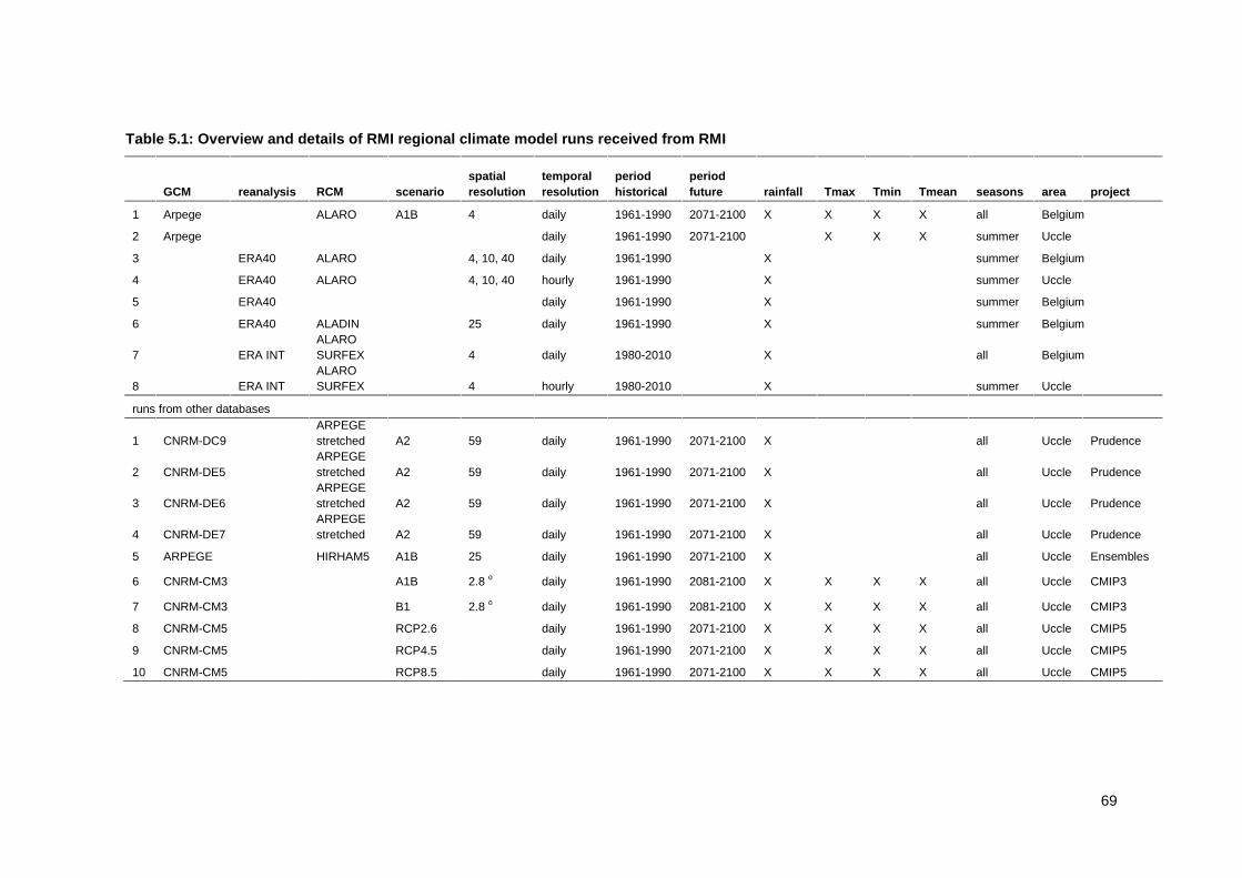
69

Table 5.1: Overview and details of RMI regional climate model runs received from RMI

GCM reanalysis RCM scenario

spatial

resolution

temporal

resolution

period

historical

period

future rainfall Tmax Tmin Tmean seasons area project

1 Arpege

ALARO A1B 4 daily 1961-1990 2071-2100 X X X X all Belgium

2 Arpege

daily 1961-1990 2071-2100

X X X summer Uccle

3

ERA40 ALARO

4, 10, 40 daily 1961-1990

X

summer Belgium

4

ERA40 ALARO

4, 10, 40 hourly 1961-1990

X

summer Uccle

5

ERA40

daily 1961-1990

X

summer Belgium

6

ERA40 ALADIN

25 daily 1961-1990

X

summer Belgium

7

ERA INT

ALARO

SURFEX

4 daily 1980-2010

X

all Belgium

8

ERA INT

ALARO

SURFEX

4 hourly 1980-2010

X

summer Uccle

runs from other databases

1 CNRM-DC9

ARPEGE

stretched A2 59 daily 1961-1990 2071-2100 X

all Uccle Prudence

2 CNRM-DE5

ARPEGE


all Uccle Prudence

3 CNRM-DE6

ARPEGE


all Uccle Prudence

4 CNRM-DE7

ARPEGE


all Uccle Prudence

5 ARPEGE

HIRHAM5 A1B 25 daily 1961-1990 2071-2100 X

all Uccle Ensembles

6 CNRM-CM3

A1B 2.8 o daily 1961-1990 2081-2100 X X X X all Uccle CMIP3

7 CNRM-CM3

B1 2.8 o daily 1961-1990 2081-2100 X X X X all Uccle CMIP3

8 CNRM-CM5

RCP2.6

daily 1961-1990 2071-2100 X X X X all Uccle CMIP5

9 CNRM-CM5

RCP4.5


10 CNRM-CM5

RCP8.5


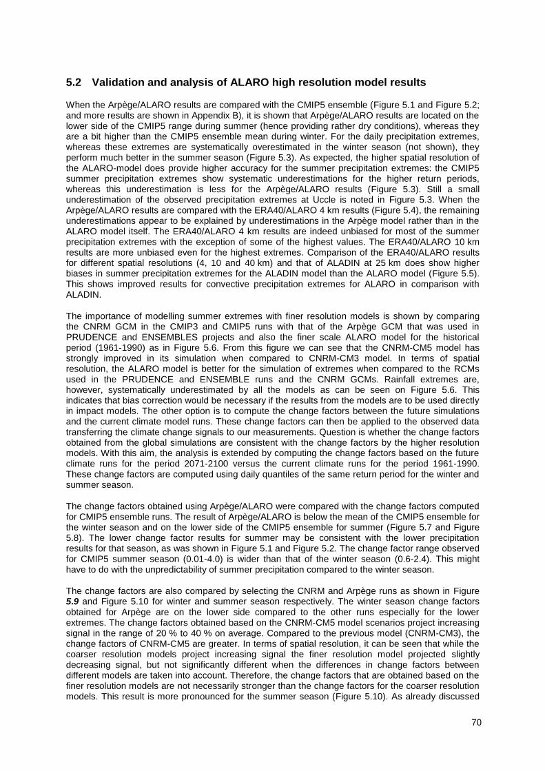
70

5.2 Validation and analysis of ALARO high resolution model results

When the Arpège/ALARO results are compared with the CMIP5 ensemble (Figure 5.1 and Figure 5.2; and more results are shown in Appendix B), it is shown that Arpège/ALARO results are located on the lower side of the CMIP5 range during summer (hence providing rather dry conditions), whereas they are a bit higher than the CMIP5 ensemble mean during winter. For the daily precipitation extremes, whereas these extremes are systematically overestimated in the winter season (not shown), they perform much better in the summer season (Figure 5.3). As expected, the higher spatial resolution of the ALARO-model does provide higher accuracy for the summer precipitation extremes: the CMIP5 summer precipitation extremes show systematic underestimations for the higher return periods, whereas this underestimation is less for the Arpège/ALARO results (Figure 5.3). Still a small underestimation of the observed precipitation extremes at Uccle is noted in Figure 5.3. When the Arpège/ALARO results are compared with the ERA40/ALARO 4 km results (Figure 5.4), the remaining underestimations appear to be explained by underestimations in the Arpège model rather than in the ALARO model itself. The ERA40/ALARO 4 km results are indeed unbiased for most of the summer precipitation extremes with the exception of some of the highest values. The ERA40/ALARO 10 km results are more unbiased even for the highest extremes. Comparison of the ERA40/ALARO results for different spatial resolutions (4, 10 and 40 km) and that of ALADIN at 25 km does show higher biases in summer precipitation extremes for the ALADIN model than the ALARO model (Figure 5.5). This shows improved results for convective precipitation extremes for ALARO in comparison with ALADIN.

The importance of modelling summer extremes with finer resolution models is shown by comparing the CNRM GCM in the CMIP3 and CMIP5 runs with that of the Arpège GCM that was used in PRUDENCE and ENSEMBLES projects and also the finer scale ALARO model for the historical period (1961-1990) as in Figure 5.6. From this figure we can see that the CNRM-CM5 model has strongly improved in its simulation when compared to CNRM-CM3 model. In terms of spatial resolution, the ALARO model is better for the simulation of extremes when compared to the RCMs used in the PRUDENCE and ENSEMBLE runs and the CNRM GCMs. Rainfall extremes are, however, systematically underestimated by all the models as can be seen on Figure 5.6. This indicates that bias correction would be necessary if the results from the models are to be used directly in impact models. The other option is to compute the change factors between the future simulations and the current climate model runs. These change factors can then be applied to the observed data transferring the climate change signals to our measurements. Question is whether the change factors obtained from the global simulations are consistent with the change factors by the higher resolution models. With this aim, the analysis is extended by computing the change factors based on the future climate runs for the period 2071-2100 versus the current climate runs for the period 1961-1990. These change factors are computed using daily quantiles of the same return period for the winter and summer season.

The change factors obtained using Arpège/ALARO were compared with the change factors computed for CMIP5 ensemble runs. The result of Arpège/ALARO is below the mean of the CMIP5 ensemble for the winter season and on the lower side of the CMIP5 ensemble for summer (Figure 5.7 and Figure 5.8). The lower change factor results for summer may be consistent with the lower precipitation results for that season, as was shown in Figure 5.1 and Figure 5.2. The change factor range observed for CMIP5 summer season (0.01-4.0) is wider than that of the winter season (0.6-2.4). This might have to do with the unpredictability of summer precipitation compared to the winter season.

The change factors are also compared by selecting the CNRM and Arpège runs as shown in Figure 5.9 and Figure 5.10 for winter and summer season respectively. The winter season change factors obtained for Arpège are on the lower side compared to the other runs especially for the lower extremes. The change factors obtained based on the CNRM-CM5 model scenarios project increasing signal in the range of 20 % to 40 % on average. Compared to the previous model (CNRM-CM3), the change factors of CNRM-CM5 are greater. In terms of spatial resolution, it can be seen that while the coarser resolution models project increasing signal the finer resolution model projected slightly decreasing signal, but not significantly different when the differences in change factors between different models are taken into account. Therefore, the change factors that are obtained based on the finer resolution models are not necessarily stronger than the change factors for the coarser resolution models. This result is more pronounced for the summer season (Figure 5.10). As already discussed

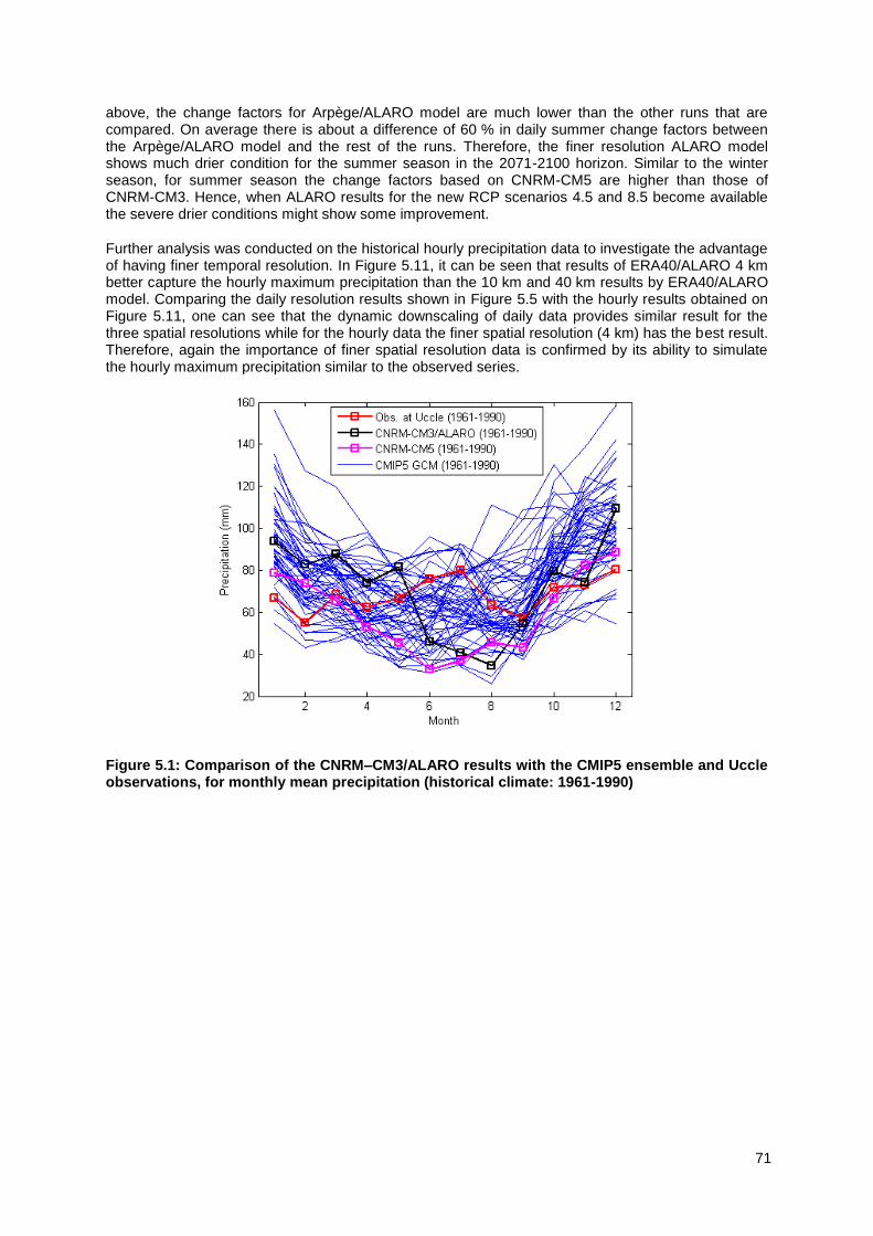
71

above, the change factors for Arpège/ALARO model are much lower than the other runs that are compared. On average there is about a difference of 60 % in daily summer change factors between the Arpège/ALARO model and the rest of the runs. Therefore, the finer resolution ALARO model shows much drier condition for the summer season in the 2071-2100 horizon. Similar to the winter season, for summer season the change factors based on CNRM-CM5 are higher than those of CNRM-CM3. Hence, when ALARO results for the new RCP scenarios 4.5 and 8.5 become available the severe drier conditions might show some improvement.

Further analysis was conducted on the historical hourly precipitation data to investigate the advantage of having finer temporal resolution. In Figure 5.11, it can be seen that results of ERA40/ALARO 4 km better capture the hourly maximum precipitation than the 10 km and 40 km results by ERA40/ALARO model. Comparing the daily resolution results shown in Figure 5.5 with the hourly results obtained on Figure 5.11, one can see that the dynamic downscaling of daily data provides similar result for the three spatial resolutions while for the hourly data the finer spatial resolution (4 km) has the best result. Therefore, again the importance of finer spatial resolution data is confirmed by its ability to simulate the hourly maximum precipitation similar to the observed series.

Figure 5.1: Comparison of the CNRM–CM3/ALARO results with the CMIP5 ensemble and Uccle observations, for monthly mean precipitation (historical climate: 1961-1990)

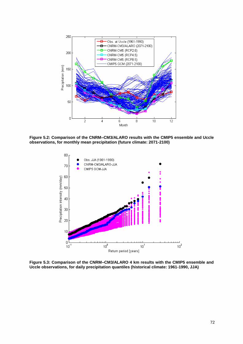
72

Figure 5.2: Comparison of the CNRM–CM3/ALARO results with the CMIP5 ensemble and Uccle observations, for monthly mean precipitation (future climate: 2071-2100)

Figure 5.3: Comparison of the CNRM–CM3/ALARO 4 km results with the CMIP5 ensemble and Uccle observations, for daily precipitation quantiles (historical climate: 1961-1990, JJA)

73

Figure 5.4: Comparison of the ERA40/ALARO 4km results with the CMIP5 ensemble and Uccle observations, for daily precipitation quantiles (historical climate: 1961-1990, JJA)

Figure 5.5: Comparison of the ERA40/ALARO 4, 10, 40 km and ERA40/ALADIN 25 km results with ERA40 and Uccle observations, for daily precipitation quantiles (historical climate: 1961-1990, JJA)

74

Figure 5.6: Comparison of the CNRM–CM3/ALARO 4 km results with the CMIP3 and CMIP5 CNRM runs, PRUDENCE and ENSEMBLES RCMs and Uccle observations, for daily precipitation quantiles (historical climate: 1961-1990, JJA)

Figure 5.7: Comparison of CNRM–CM3/ALARO change factors for 2071-2100 vs. 1961-1990 with those of the CMIP5 ensemble for the winter season (DJF)

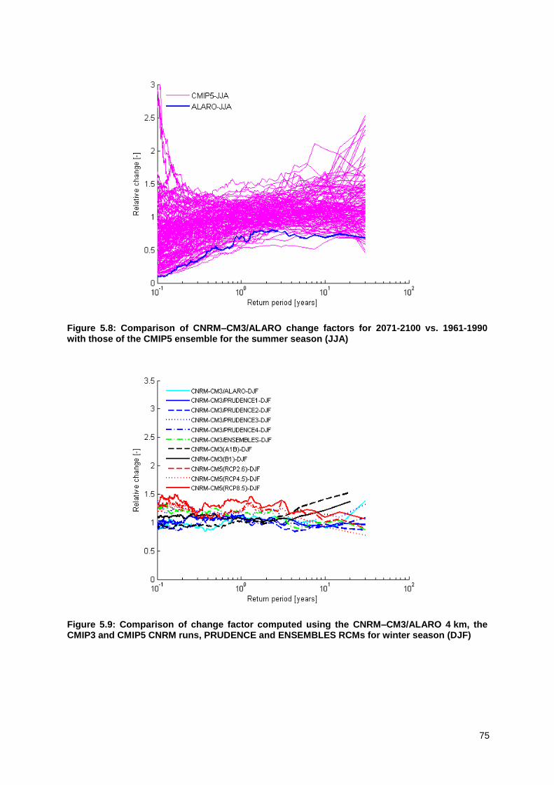
75

Figure 5.8: Comparison of CNRM–CM3/ALARO change factors for 2071-2100 vs. 1961-1990 with those of the CMIP5 ensemble for the summer season (JJA)

Figure 5.9: Comparison of change factor computed using the CNRM–CM3/ALARO 4 km, the CMIP3 and CMIP5 CNRM runs, PRUDENCE and ENSEMBLES RCMs for winter season (DJF)

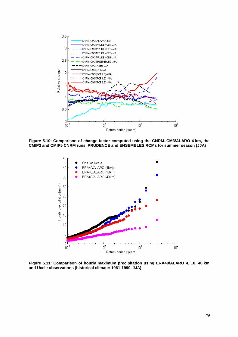
76

Figure 5.10: Comparison of change factor computed using the CNRM–CM3/ALARO 4 km, the CMIP3 and CMIP5 CNRM runs, PRUDENCE and ENSEMBLES RCMs for summer season (JJA)

Figure 5.11: Comparison of hourly maximum precipitation using ERA40/ALARO 4, 10, 40 km and Uccle observations (historical climate: 1961-1990, JJA)

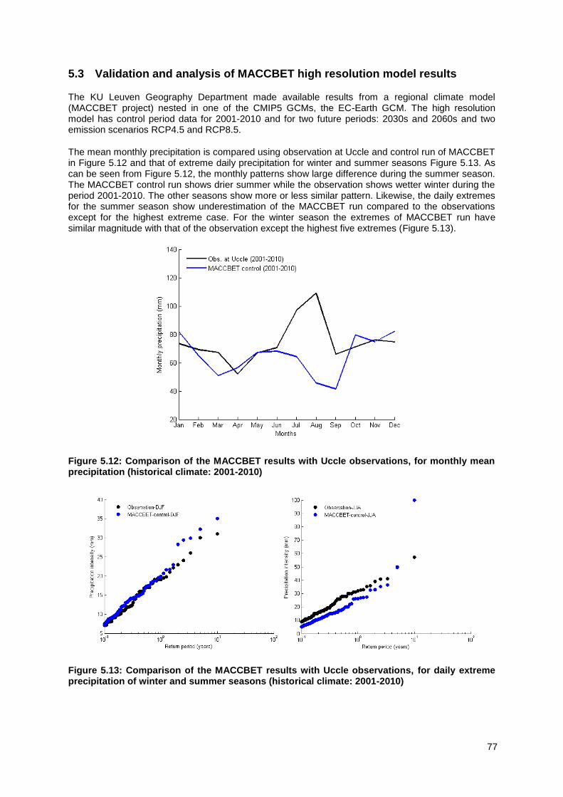
77

5.3 Validation and analysis of MACCBET high resolution model results

The KU Leuven Geography Department made available results from a regional climate model (MACCBET project) nested in one of the CMIP5 GCMs, the EC-Earth GCM. The high resolution model has control period data for 2001-2010 and for two future periods: 2030s and 2060s and two emission scenarios RCP4.5 and RCP8.5.

The mean monthly precipitation is compared using observation at Uccle and control run of MACCBET in Figure 5.12 and that of extreme daily precipitation for winter and summer seasons Figure 5.13. As can be seen from Figure 5.12, the monthly patterns show large difference during the summer season. The MACCBET control run shows drier summer while the observation shows wetter winter during the period 2001-2010. The other seasons show more or less similar pattern. Likewise, the daily extremes for the summer season show underestimation of the MACCBET run compared to the observations except for the highest extreme case. For the winter season the extremes of MACCBET run have similar magnitude with that of the observation except the highest five extremes (Figure 5.13).

Figure 5.12: Comparison of the MACCBET results with Uccle observations, for monthly mean precipitation (historical climate: 2001-2010)

Figure 5.13: Comparison of the MACCBET results with Uccle observations, for daily extreme precipitation of winter and summer seasons (historical climate: 2001-2010)

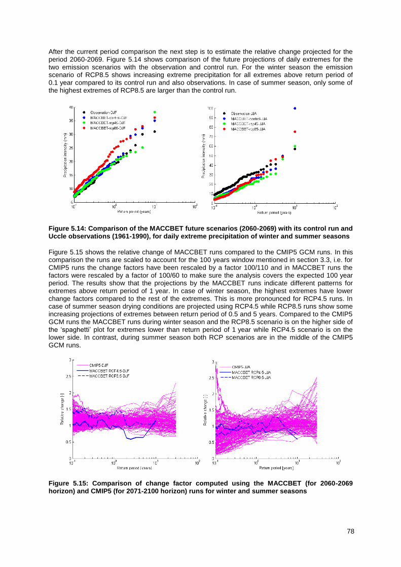
78

After the current period comparison the next step is to estimate the relative change projected for the period 2060-2069. Figure 5.14 shows comparison of the future projections of daily extremes for the two emission scenarios with the observation and control run. For the winter season the emission scenario of RCP8.5 shows increasing extreme precipitation for all extremes above return period of 0.1 year compared to its control run and also observations. In case of summer season, only some of the highest extremes of RCP8.5 are larger than the control run.

Figure 5.14: Comparison of the MACCBET future scenarios (2060-2069) with its control run and Uccle observations (1961-1990), for daily extreme precipitation of winter and summer seasons

Figure 5.15 shows the relative change of MACCBET runs compared to the CMIP5 GCM runs. In this comparison the runs are scaled to account for the 100 years window mentioned in section 3.3, i.e. for CMIP5 runs the change factors have been rescaled by a factor 100/110 and in MACCBET runs the factors were rescaled by a factor of 100/60 to make sure the analysis covers the expected 100 year period. The results show that the projections by the MACCBET runs indicate different patterns for extremes above return period of 1 year. In case of winter season, the highest extremes have lower change factors compared to the rest of the extremes. This is more pronounced for RCP4.5 runs. In case of summer season drying conditions are projected using RCP4.5 while RCP8.5 runs show some increasing projections of extremes between return period of 0.5 and 5 years. Compared to the CMIP5 GCM runs the MACCBET runs during winter season and the RCP8.5 scenario is on the higher side of the ‘spaghetti’ plot for extremes lower than return period of 1 year while RCP4.5 scenario is on the lower side. In contrast, during summer season both RCP scenarios are in the middle of the CMIP5 GCM runs.

Figure 5.15: Comparison of change factor computed using the MACCBET (for 2060-2069 horizon) and CMIP5 (for 2071-2100 horizon) runs for winter and summer seasons

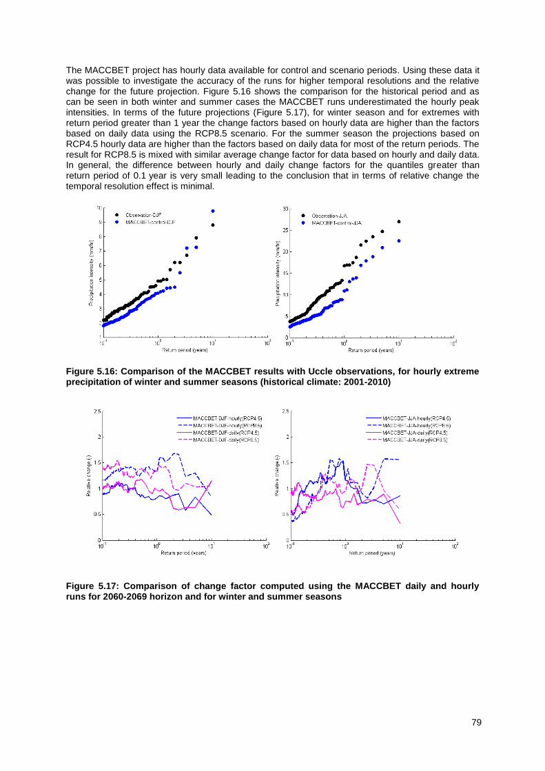
79

The MACCBET project has hourly data available for control and scenario periods. Using these data it was possible to investigate the accuracy of the runs for higher temporal resolutions and the relative change for the future projection. Figure 5.16 shows the comparison for the historical period and as can be seen in both winter and summer cases the MACCBET runs underestimated the hourly peak intensities. In terms of the future projections (Figure 5.17), for winter season and for extremes with return period greater than 1 year the change factors based on hourly data are higher than the factors based on daily data using the RCP8.5 scenario. For the summer season the projections based on RCP4.5 hourly data are higher than the factors based on daily data for most of the return periods. The result for RCP8.5 is mixed with similar average change factor for data based on hourly and daily data. In general, the difference between hourly and daily change factors for the quantiles greater than return period of 0.1 year is very small leading to the conclusion that in terms of relative change the temporal resolution effect is minimal.

Figure 5.16: Comparison of the MACCBET results with Uccle observations, for hourly extreme precipitation of winter and summer seasons (historical climate: 2001-2010)

Figure 5.17: Comparison of change factor computed using the MACCBET daily and hourly runs for 2060-2069 horizon and for winter and summer seasons

80

5.4 Spatial differences

Previous investigations were done for the GCM and RCM results for the grid cell covering the Uccle station. It is, however, important to also study the regional differences across the country or region. In the CCI-HYDR climate scenarios, differences in climate scenarios were identified and defined for two regions: the inland region and the coastal area (‘polders’). The coarse-scale CMIP5 runs do not allow such regional analysis, because Belgium is covered by few grid cells only. The study of regional differences hence should be done based on the high resolution models. Such regional analysis was done as part of the MIRA 2015 study by Beullens & van Lipzig (2015).

For the ALARO model by RMI (De Troch et al., 2014), Source : De Troch et al. (2014)

Figure 5.18 shows the regional analysis at seasonal scale. The results show that for the winter period increase in precipitation is projected for both inland and coastal areas. For the other three seasons, decrease in precipitation is projected for the end of the century. The Flanders area shows similar magnitude of decrease in precipitation for inland and coastal areas. However, in the inland areas slight differences can be noted between the more urbanized central region largely covered by the triangle formed by the cities Brussels, Antwerp, Gent and the other areas (coastal area and Kempen-Limburg).

When the analysis is done for all available high-resolution climate models for Belgium (Beullens & van Lipzig, 2015), then the ensemble based spatial patterns of

Source: Beullens & van Lipzig (2015)

Figure 5.19 are obtained. The winter season shows higher increases in the winter season for the coastal region, whereas the summer season shows stronger decreases for that region. The higher increases in winter rainfall for the coastal region is consistent with what was found in the CCI-HYDR project, but the changes in summer rainfall are not consistent with these old scenarios (less dry conditions were found for the coastal area in the CCI-HYDR project).

Source : De Troch et al. (2014)

81

Figure 5.18: 30-year (2071-2100) seasonal mean precipitation anomaly relative to the 30-year mean of the period 1961-1990


Figure 5.19: Regional differences across Belgium of the mean seasonal rainfall change over 100 years for the winter (left figure) and summer (right figure), based on the available ensemble of high-resolution climate runs

For temperature, Beullens & van Lipzig (2015) show small regional differences in mean annual temperature changes across temperature changes across Flanders: lower temperature increase along the Belgian coast (in de ‘polders’ area) (Source: ‘polders’ area) (Source: Beullens & van Lipzig (2015)

Figure 5.20). Also for temperature extremes (number of days with temperature higher than 25 °C or lower than 0 °C, the coastal area shows lower changes. For the inland Flanders’ region, no significant differences are found for the mean annual temperature change, but for the changes in temperature extremes, some regional differences are noted (Source: Beullens & van Lipzig (2015)

Figure 5.21): higher changes in the sandy region of the ‘kempen’.

However, because the number of high resolution model runs is still limited, these regional differences have to be applied with care.

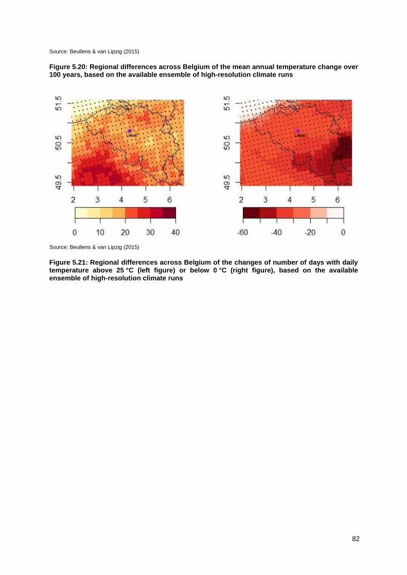
82


Figure 5.20: Regional differences across Belgium of the mean annual temperature change over 100 years, based on the available ensemble of high-resolution climate runs


Figure 5.21: Regional differences across Belgium of the changes of number of days with daily temperature above 25 °C (left figure) or below 0 °C (right figure), based on the available ensemble of high-resolution climate runs

83

5.5 Conclusions

Based on these high resolution regional Belgian climate model runs, the following research questions could be answered:

Based on the comparison between the climate model results from the coarse scale to the small scale: global -> European regional -> fine-scale Belgium 40 km -> … -> 10 km -> 4 km (for the same global and regional models as boundary conditions): the precipitation results come closer to the observations if the spatial scale is reduced (because convection is more explicitly resolved). The high resolution ALARO model indeed provides improved (unbiased) results for summer precipitation extremes in Belgium.

The global model that RMI used as boundary condition for their fine-scale runs is located on the lower side of the entire set of CMIP5 or CMIP3 runs.

If the global and/or regional model is replaced by ERA40 historical re-analysis data, the model results come closer to the observations. This gave us an idea about the bias in the global or regional results, and also of the quality of the ERA40 re-analysis data.

If the CMIP5 and CMIP3 runs are compared for the same global model (e.g. CNRM), we see differences: the CMIP5 run comes closer to the observations. This indicates that the new generation GCM comes closer to the observations; hence it is good to see that the models improve from the old to the new generation.

ALARO model is better than ALADIN for dynamic downscaling of precipitation in Belgium.

For summer season, MACCBET future projections are not as dry as that of ALARO model.

For higher temporal resolution, i.e. hourly data, MACCBET control period results underestimated both winter and summer season rainfall extremes while in the case of daily data only the summer season extremes are underestimated.

The high resolution climate models could also be applied to study regional differences in rainfall and temperature changes across the Flanders region. Some patterns, such as the higher increase in winter rainfall along the coastal area, is consistent with the regional differences applied for the CCI-HYDR scenarios, but also regional differences are inconsistent or less clear. Because the number of high resolution model runs is still limited, the regional differences have to be applied with care.

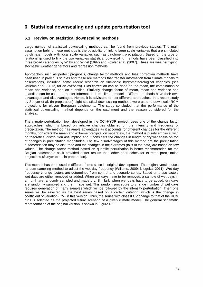
84

6 Statistical downscaling and update perturbation tool

6.1 Review on statistical downscaling methods

Large number of statistical downscaling methods can be found from previous studies. The main assumption behind these methods is the possibility of linking large scale variables that are simulated by climate models with local scale variables such as catchment precipitation. Based on the type of relationship used to link the two variables statistical downscaling methods have been classified into three broad categories by Wilby and Wigel (1997) and Fowler et al. (2007). These are weather typing, stochastic weather generators and regression methods.

Approaches such as perfect prognosis, change factor methods and bias correction methods have been used in previous studies and these are methods that transfer information from climate models to observations, including some recent research on fine-scale hydrometeorological variables (see Willems et al., 2012, for an overview). Bias correction can be done on the mean, the combination of mean and variance, and on quantiles. Similarly change factor of mean, mean and variance and quantiles can be used to transfer information from climate models. Different methods have their own advantages and disadvantages. Hence, it is advisable to test different approaches. In a recent study by Sunyer et al. (in preparation) eight statistical downscaling methods were used to downscale RCM projections for eleven European catchments. The study concluded that the performance of the statistical downscaling method depends on the catchment and the season considered for the analysis.

The climate perturbation tool, developed in the CCI-HYDR project, uses one of the change factor approaches, which is based on relative changes obtained on the intensity and frequency of precipitation. The method has ample advantages as it accounts for different changes for the different months, considers the mean and extreme precipitation separately, the method is purely empirical with no theoretical distribution assumption and it considers the changes in length of dry/wet spells on top of changes in precipitation magnitudes. The few disadvantages of this method are the precipitation autocorrelation may be disturbed and the changes in the extremes (tails of the data) are based on few values. The change factor method based on quantile perturbation is better recommended for the Belgian catchments as it provided better results than other approaches for extreme precipitation projections (Sunyer et al., in preparation).

This method has been used in different forms since its original development. The original version uses random sampling method to adjust the wet day frequency (Willems, 2009; Ntegeka, 2011). Wet-day frequency change factors are determined from control and scenario series. Based on these factors wet days are either removed or added. When wet days have to be removed, a sample of wet days in a month are randomly sampled and made dry. Similarly when wet days have to be added, dry days are randomly sampled and then made wet. This random procedure to change number of wet days requires generation of many samples which will be followed by the intensity perturbation. Then one series will be selected as the best series based on a certain criterion, which is the change in coefficient of variation (CV) in this version. Thus, the series with closest CV change to that of the RCM runs is selected as the projected future scenario of a given climate model. The general schematic representation of the original version is shown in Figure 6.1.

85

Month i Month i Month i

Wet day frequency

perturbation

Wet day intensity

perturbation

Combined perturbation

Time

series

Time

series

Figure 6.1: General methodology of precipitation perturbation

Mora et al. (2013) made some developments on this downscaling method. The advancement is in the application of relative and absolute change in precipitation intensity. The addition of absolute change is initiated due to the following reasons: application of change factor (obtained by relative change) on observed values that are close to zero will result in similar small values even if the factor is high enough. Similarly, when control values are close to zero the change factor obtained will be very high and the application of these factors might lead to unrealistic excessive precipitation values in the future scenarios. Therefore, for precipitation values lower than a certain threshold the application of absolute change factors is considered (Figure 6.2). The values above the chosen threshold will be perturbed using the relative change factors.

Figure 6.2: Illustration of absolute and relative change factor calculation

Additional improvement was also done on the method used to adjust the number of wet days. In the original version, the random sampling method was used. It was suggested that instead of the random sampling, the adding and removing of wet days to be performed on the longest wet or dry spells (Willems and Vrac, 2011). This method was suggested to avoid the addition/removal of a wet day in unrealistic position. Other recent improvements are the use of probability distributions for describing precipitation extremes for the higher return periods rather than the empirical values directly obtained from the climate model simulations (Willems, 2013). This avoids that the random variations in empirical extremes affect the change factors.

In Sunyer et al. (2014) eight statistical downscaling methods were used to obtain downscaled RCM projections at the catchment scale for eleven catchments in Europe. One of these catchments was the Grote Nete and the quantile perturbation method was among the methods that were tested. The statistical methods were grouped as bias correction (BC) and change factor (CF) methods and

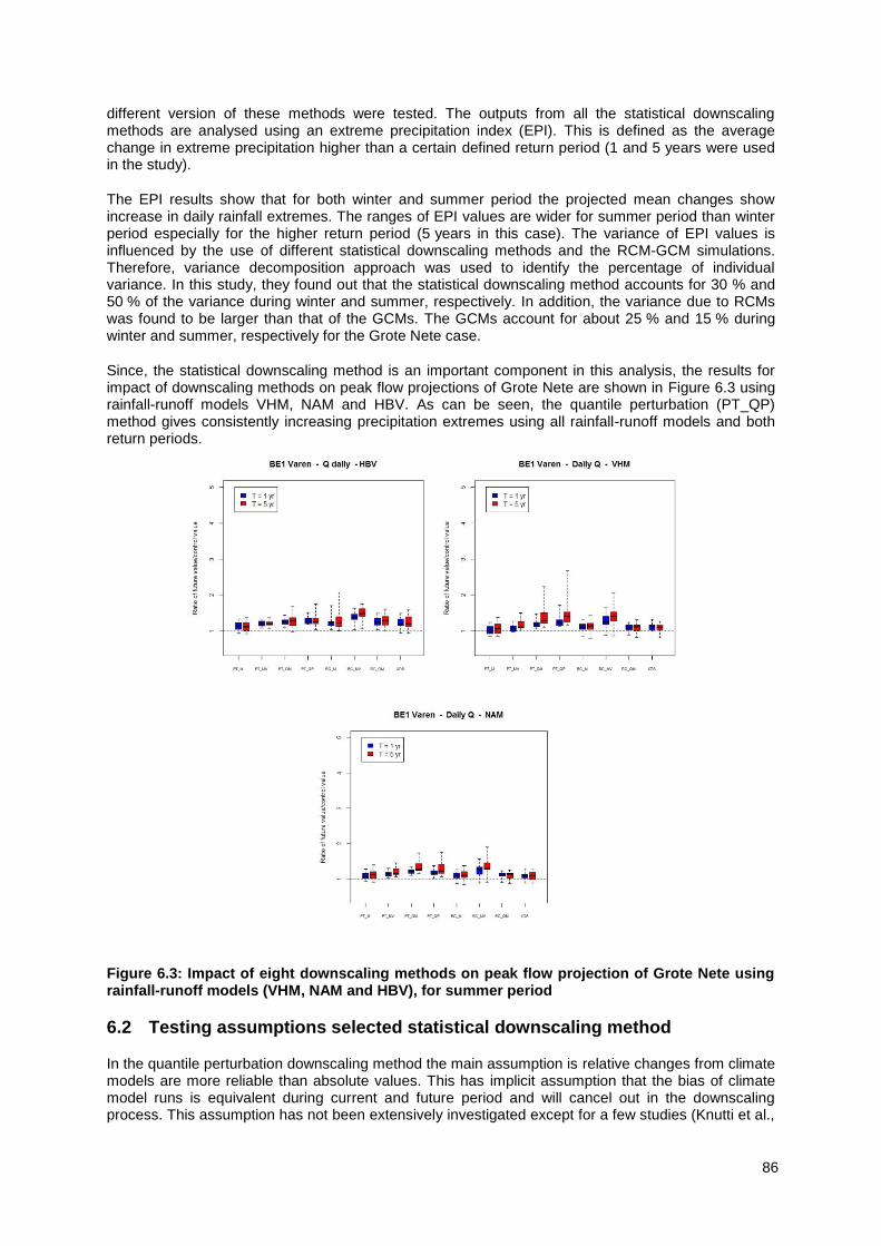
86

different version of these methods were tested. The outputs from all the statistical downscaling methods are analysed using an extreme precipitation index (EPI). This is defined as the average change in extreme precipitation higher than a certain defined return period (1 and 5 years were used in the study).

The EPI results show that for both winter and summer period the projected mean changes show increase in daily rainfall extremes. The ranges of EPI values are wider for summer period than winter period especially for the higher return period (5 years in this case). The variance of EPI values is influenced by the use of different statistical downscaling methods and the RCM-GCM simulations. Therefore, variance decomposition approach was used to identify the percentage of individual variance. In this study, they found out that the statistical downscaling method accounts for 30 % and 50 % of the variance during winter and summer, respectively. In addition, the variance due to RCMs was found to be larger than that of the GCMs. The GCMs account for about 25 % and 15 % during winter and summer, respectively for the Grote Nete case.

Since, the statistical downscaling method is an important component in this analysis, the results for impact of downscaling methods on peak flow projections of Grote Nete are shown in Figure 6.3 using rainfall-runoff models VHM, NAM and HBV. As can be seen, the quantile perturbation (PT_QP) method gives consistently increasing precipitation extremes using all rainfall-runoff models and both return periods.

Figure 6.3: Impact of eight downscaling methods on peak flow projection of Grote Nete using rainfall-runoff models (VHM, NAM and HBV), for summer period

6.2 Testing assumptions selected statistical downscaling method

In the quantile perturbation downscaling method the main assumption is relative changes from climate models are more reliable than absolute values. This has implicit assumption that the bias of climate model runs is equivalent during current and future period and will cancel out in the downscaling process. This assumption has not been extensively investigated except for a few studies (Knutti et al.,

87

2010; Muerth et al., 2013), which have shown that the assumption has some basis (Ntegeka et al., 2014). Other assumptions are the climate change signals obtained from global climate models and the regional climate models are similar (at different spatial scale) and the change factors obtained from climate models are similar at different temporal scales. Although not all assumptions can be tested, some investigation could be done on some of the claims.

Based on the high resolution ALARO climate model, it is shown that for the historical period, the finer resolution ALARO results are closer to the observations than the coarse resolution model (CNRM) used as the boundary condition for that model; idem for the PRUDENCE and ENSEMBLES RCMs (Figure 6.4). Hence, we expect the future simulations to be more accurate than the coarse resolution models. In terms of future projection, the change factors obtained by the ALARO model are on the lower side when compared to the CMIP5 GCM runs (see Figure 5.7 and Figure 5.8). However, also the location of the CNRM GCM in the CMIP5 GCM ensemble has to be considered (see Figure 5.1 and Figure 5.2). When the ALARO precipitation changes are compared with the CMIP5 CNRM GCM changes (Figure 6.5), the high resolution model projects much drier conditions for summer and slightly wetter conditions for winter. The difference between the high and low resolution models thus is more considerable for summer period than for winter. However, it is not possible to draw sound conclusions using only one high resolution model. Furthermore, RMI reported the presence of inaccuracy in the algorithm for the winter period and recalculation is being done. Therefore, there is a need to re-do the analysis for winter when this recalculation becomes available.

Figure 6.4: Comparison of hourly (left) and daily (right) precipitation extremes in the summer season for the different resolution and generation climate models

Figure 6.5: Comparison of change factor computed for the different resolution and generation climate models

88

6.3 Perturbation tool

The perturbation tool developed in the CCI-HYDR projects adopts the quantile perturbation methodology in which precipitation relative changes are calculated based on the daily intensities after grouping the daily data in monthly blocks. Two relative changes are of main interest. The change in number of wet days is represented as the wet-day frequency perturbation while the change in intensity or magnitude is represented as wet-day quantile perturbation (Ntegeka et al., 2014). These factors are obtained at daily scale and are applied on daily observation data. In addition to precipitation the tool perturbs temperature and ETo series, based on the temperature and ETo changes and their correlations with precipitation changes (see section 3.3.4). These changes are computed at monthly scale unlike precipitation and applied on the daily series. The tool takes observed precipitation, temperature and ETo series as input data, and produces for each of the climate scenarios (e.g. high, mean, low) future (perturbed) series of the same length as the input series, following the method described above.

The comparison between the CCI-HYDR scenarios and that of the CMIP5 do not show significant difference in change factors for the precipitation variable. Hence, there is no need to update the tool in terms of precipitation. However, temperature and mainly ETo show significant difference for the high and mean climate scenarios. For this reason the perturbation tool is updated for these two variables based on the new change factors obtained in Section 3. The new tool was applied to the 100-year Uccle series to obtain new perturbed series. The new perturbation tool can also be applied to perturb any historical series of precipitation, temperature and/or ETo, and is freely available on: http://www.kuleuven.be/hydr/CCI-HYDR.htm.


90

References

Baguis, P., Roulin, E., Willems, P., Ntegeka, V., 2009. Climate change scenarios for precipitation and potential evapotranspiration over central Belgium. Theoretical and Applied Climatology, 99(3-4), 273-286.

Beullens, J., van Lipzig, N., 2015. Actualisatie en verfijning klimaatscenario’s tot 2100 voor Vlaanderen - Appendix 3: Ruimtelijke patronen voor België op basis van regionale klimaatmodellen (CORDEX) en een hoge resolutiemodellen (MACCBET en ALARO). Studie uitgevoerd in opdracht van de Vlaamse Milieumaatschappij,

MIRA2015 raadpleegbaar op www.milieurapport.be, KU Leuven.

Beullens, J., van Lipzig, N., De Troch, R., Termonia, P., Tabari, H., Taye, M.T., Willems, P., 2015. Actualisatie en verfijning klimaatscenario’s tot 2100 voor Vlaanderen. Studie uitgevoerd in opdracht van de Vlaamse

Milieumaatschappij, MIRA2015 raadpleegbaar op www.milieurapport.be, KU Leuven i.s.m. KMI.

Brouwers J., Peeters B., Willems P., Deckers P., De Maeyer Ph., De Sutter R., Vanneuville W., 2009. MIRA 2009: Milieuverkenning 2030, Hoofdstuk 11 ‘Klimaatverandering en waterhuishouding’, Milieurapport Vlaanderen, Vlaamse Milieumaatschappij, 283-304.

Bultot, F., Coppens, A., Dupriez, G., 1983. Estimation de l’évapotranspiration potentielle en Belgique. Publications/publicaties série/serie A, No/Nr 112, Institut Royal Météorologique de Belgique - Koninklijk Meteorologisch Instituut van België , 28 p.

De Troch, R., Giot, O., Hamdi, R., Saeed, S., Tabari, H., Taye, M.T., Termonia, P., Van Lipzig, N., Willems, P., 2014. Overview of a few regional climate models and climate scenarios for Belgium. Koninklijk Meteorologisch Instituut van België / Institut Royal Météorologique de Belgique, Wetenschappelijke en technische publicatie, 32 p.

Fowler, H. J, Blenkinsop, S. And Tebaldi, C., 2007. Linking climate change modelling to impacts studies: recent advances in downloading techniques for hydrological modelling, Int. J. Climatol., 27, 1547-1578.

Gellens-Meulenberghs, F., Gellens, D., 1992. L’évapotranspiration potentielle en Belgique : variabilité spatiale et temporelle. Publications/publicaties série/serie A, No/Nr 130, Institut Royal Météorologique de Belgique - Koninklijk Meteorologisch Instituut van België.

Knutti, R., Furrer, R., Tebaldi, C., Cermak, J., Meehl, G.A., 2010. Challenges in combining projections from multiple climate models. Journal of Climate 23, 2739–2758.

Mora, D.E., Campozano, L., Cisneros, F. Wyseure, G. and Willems, P., 2014. Climate changes of hydrometeorological and hydrological extremes in the Paute basin, Ecuadorean Andes, Hydrol. Earth Syst. Sci., 18, 1-18.

Moss, R.H., Babiker, M., Brinkman, S., Calvo, E., Carter, T., Edmonds, J., Elgizouli, I., Emori, S., Erda, L., Hibbard, K., Jones, R., Kainuma, M., Kelleher, J., Lamarque, J-F., Manning, M., Matthews, B., Meehl, J., Meyer, L., Mitchell, J., Nakicenovic, N., O’Neill, B., Pichs, R., Riahi, K., Rose, S., Runci, P., Stouffer, R., van Vuuren, D., Weyant, J., Wilbanks, T., van Ypersele, J-P., Zurek, M., 2008. Towards new scenarios for analysis of emissions, climate change, impacts, and response strategies. Intergovernmental Panel on Climate Change Secretariat, Geneva, Switzerland, 132 p.

Muerth, M.J., Gauvin St-Denis, B., Ricard, S., Velázquez, J.A., Schmid, J., Minville, M., Caya, D., Chaumont, D., Ludwig, R., Turcotte, R., 2013. On the need for bias correction in regional climate scenarios to assess climate change impacts on river runoff. Hydrology and Earth System Sciences 17 (3), 1189–1204.

Nakicenovic, N., Swart, R. (Eds.), 2000. Special Report on Emissions Scenarios (SRES). A special report of the IPCC Working Group III, Cambridge University Press, Cambridge, UK, 599 p.

Nakicenovic, N., Alcamo, J., Davis, G., de Vries, B., Fenhann, J., Gaffin, S., Gregory, K., Grubler, A., 2000. Special Report on Emissions Scenarios: A Special Report of Working Group III of the Intergovernmental Panel on Climate Change, Cambridge University Press, Cambridge, UK, 599 p.

Ntegeka, V. 2011. Assessment of the observed and future climate variability and change in hydroclimatic and hydrological extremes. PhD thesis, KU Leuven, Belgium.

Ntegeka, V., Roulin, E., Baguis, P., Willems, P., 2014. Developing tailored climate change scenarios for hydrological impact assessments. Journal of Hydrology, 508C, 307-321.

Penman, H.L., 1948. Natural evapotranspiration from open water, bare soil and grass. Proc. Roy. Soc. London, A193, 126-146.

Peters, G.P., Andrew, R.M., Boden, T., Canadell, J.G., Ciais, P., Quéré, C. Le, Marland, G., Raupach, M.R., Wilson, C., 2013. The challenge to keep global warming below 2 °C. Nature Clim. Change, 3, 4-6.



91

Sunyer, M.A., Hundecha, Y., Lawrence, D., Madsen, H., Willems, P., Martinkova, M., Vermoor, K., Bürger, G., Hanel, M., Kriaučiūnienė, J., Loukas, A., Osuch, M., Yücel, I., 2014. ‘Inter-comparison of statistical downscaling methods for projection of extreme precipitation in Europe’, Hydrology and Earth System Sciences Discussions, 11, 6167-6214.

Tabari, H., Taye, M.T., Willems, P., 2014. Bijsturing klimaatscenario’s voor hydrologische & hydrodynamische impactanalyse - Statistische analyse nieuwe CMIP5 klimaatmodelruns voor België, KU Leuven voor Vlaamse Milieumaatschappij – Afdeling Operationeel Waterbeheer, augustus 2014.

Ward, J.D., Werner, A.D., Nel, W.P., Beecham, S., 2011. The influence of constrained fossil fuel emissions scenarios on climate and water resource projections. Hydrology and Earth System Sciences, 15(6), 879-1893.

Wilby, R.L., and Wigley, T. M. L.,1997. Downscaling general circulation model output: a review of methods and limitations. Progress in Physical Geography, 21(4), 530–548.

Willems, P., 2009. Actualisatie en extrapolatie van hydrologische parameters in de nieuwe Code van Goede Praktijk voor het Ontwerp van Rioleringssystemen. Eindrapport voor VMM-Afdeling Operationeel Waterbeheer, september 2009, 79 p.

Willems, P., 2011. Evaluatie en actualisatie van de IDF-neerslagstatistieken te Ukkel’, Aanvulling bij de studie ‘Actualisatie en extrapolatie van hydrologische parameters in de nieuwe Code van Goede Praktijk voor het Ontwerp van Rioleringssystemen (KU Leuven voor VMM, sept. 2009)’, oktober 2011, 14 p.

Willems, P., 2013. Revision of urban drainage design rules after assessment of climate change impacts on precipitation extremes at Uccle, Belgium. Journal of Hydrology, 496, 166–177.

Willems, P., Deckers, P., De Maeyer, Ph., De Sutter, R., Vanneuville, W., Brouwers, J., Peeters, B., 2009. Klimaatverandering en waterhuishouding, Wetenschappelijk rapport, MIRA 2009 & NARA 2009, Vlaamse Milieumaatschappij en Instituut voor Natuur- en Bosonderzoek, www.milieurapport.be en www.nara.be.

Willems, P., De Bruyn, L., Maes, D., Brouwers, J., Peeters, B., 2009. NARA 2009: Natuurverkenning 2030, Natuurrapport Vlaanderen, Hoofdstuk 2 ‘Klimaat’, Instituut voor Natuur- en Bosonderzoek, rapport INBO.M.2009.7, 55-66.

Willems, P., Ntegeka, V., Baguis, P., Roulin, E., 2010. Climate change impact on hydrological extremes along rivers and urban drainage systems. Final report for Belgian Science Policy Office, KU Leuven - Hydraulics Section & Royal Meteorological Institute of Belgium, December 2010, 110 p.; http://www.kuleuven.be/hydr/CCI-HYDR.htm.

Willems, P., Vrac, M., 2011. Statistical precipitation downscaling for small-scale hydrological impact investigations of climate change. Journal of Hydrology, 402, 193-205.

Willems, P., Arnbjerg-Nielsen, K., Olsson, J., Nguyen, V.T.V., 2012. Climate change impact assessment on urban rainfall extremes and urban drainage: methods and shortcomings. Atmospheric Research, 103, 106-118.

Willems, P., Olsson, J., Arnbjerg-Nielsen, K., Beecham, S., Pathirana, A., Bülow Gregersen, I., Madsen, H., Nguyen, V-T-V., 2012. Impacts of climate change on rainfall extremes and urban drainage. IWA Publishing, 252p., Paperback Print ISBN 9781780401256; Ebook ISBN 9781780401263.


http://www.nara.be/



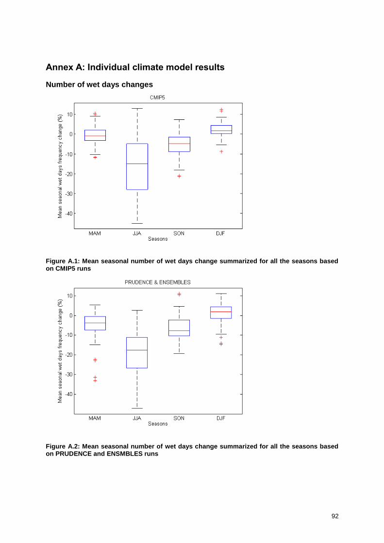
92

Annex A: Individual climate model results

Number of wet days changes

Figure A.1: Mean seasonal number of wet days change summarized for all the seasons based on CMIP5 runs

Figure A.2: Mean seasonal number of wet days change summarized for all the seasons based on PRUDENCE and ENSMBLES runs

93

Mean seasonal precipitation changes

Figure A.3: Mean seasonal precipitation change summarized for all the seasons based on CMIP5 runs

Figure A.4: Mean seasonal precipitation change summarized for all the seasons based on PRUDENCE and ENSMBLES runs

94

Monthly change factors of ‘best’ models

Figure A.5: High, mean and low scenarios extracted from the ‘best’ CMIP5 GCM runs

Wet day precipitation quantiles changes

Figure A.6: Wet day change factors calculated based on control (1961-1990) and scenario (2071-2100) runs versus return periods, for RCP2.6 scenarios and one representative month from each season

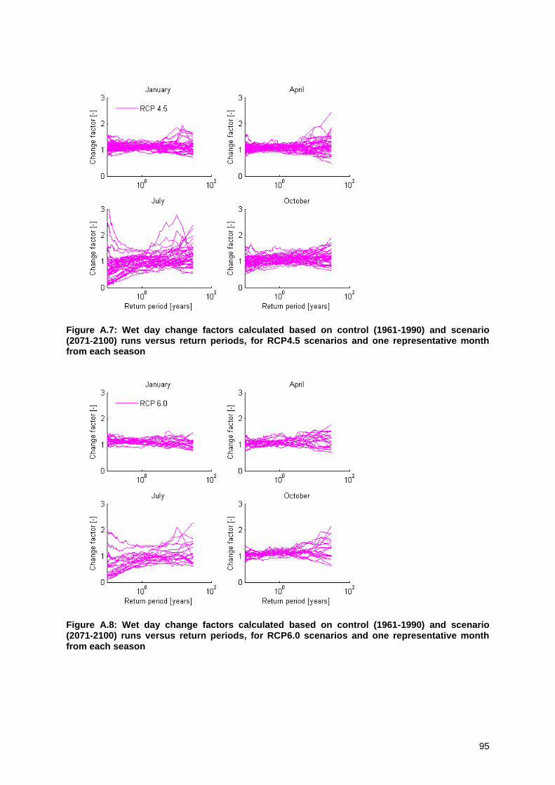
95



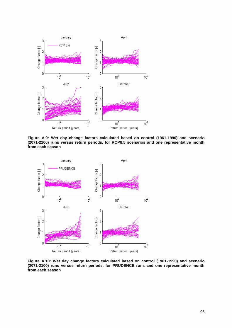
96


Figure A.10: Wet day change factors calculated based on control (1961-1990) and scenario (2071-2100) runs versus return periods, for PRUDENCE runs and one representative month from each season

97

Figure A.11: Wet day change factors calculated based on control (1961-1990) and scenario (2071-2100) runs versus return periods, for ENSEMBLES runs and one representative month from each season

98

Annex B: Climate model results versus observations

Daily precipitation quantiles: per month

Control runs (1961-1990)

Scenario runs (2071-2100)

Figure B.1: Wet day precipitation intensities vs. return period: validation of CMIP5 GCM runs based on Uccle historical observations (1961-1990) (left) and comparison with CMIP5 GCM scenario runs (2071-2100) (right), for January to March

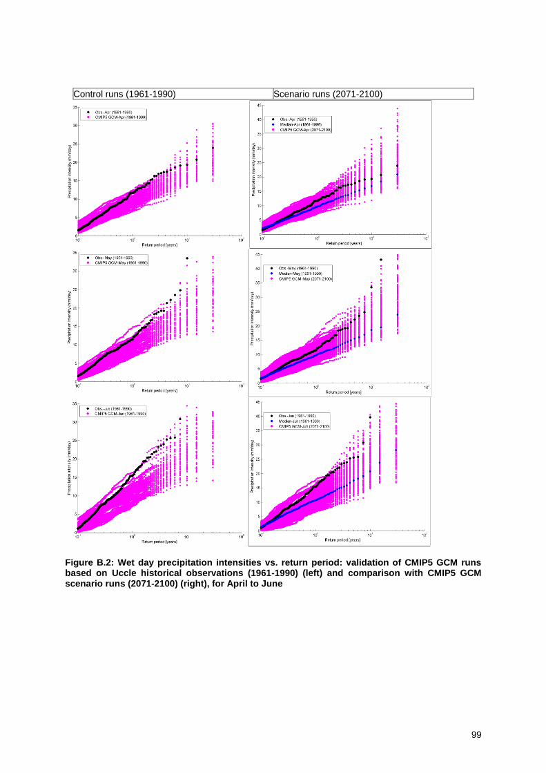
99



Figure B.2: Wet day precipitation intensities vs. return period: validation of CMIP5 GCM runs based on Uccle historical observations (1961-1990) (left) and comparison with CMIP5 GCM scenario runs (2071-2100) (right), for April to June

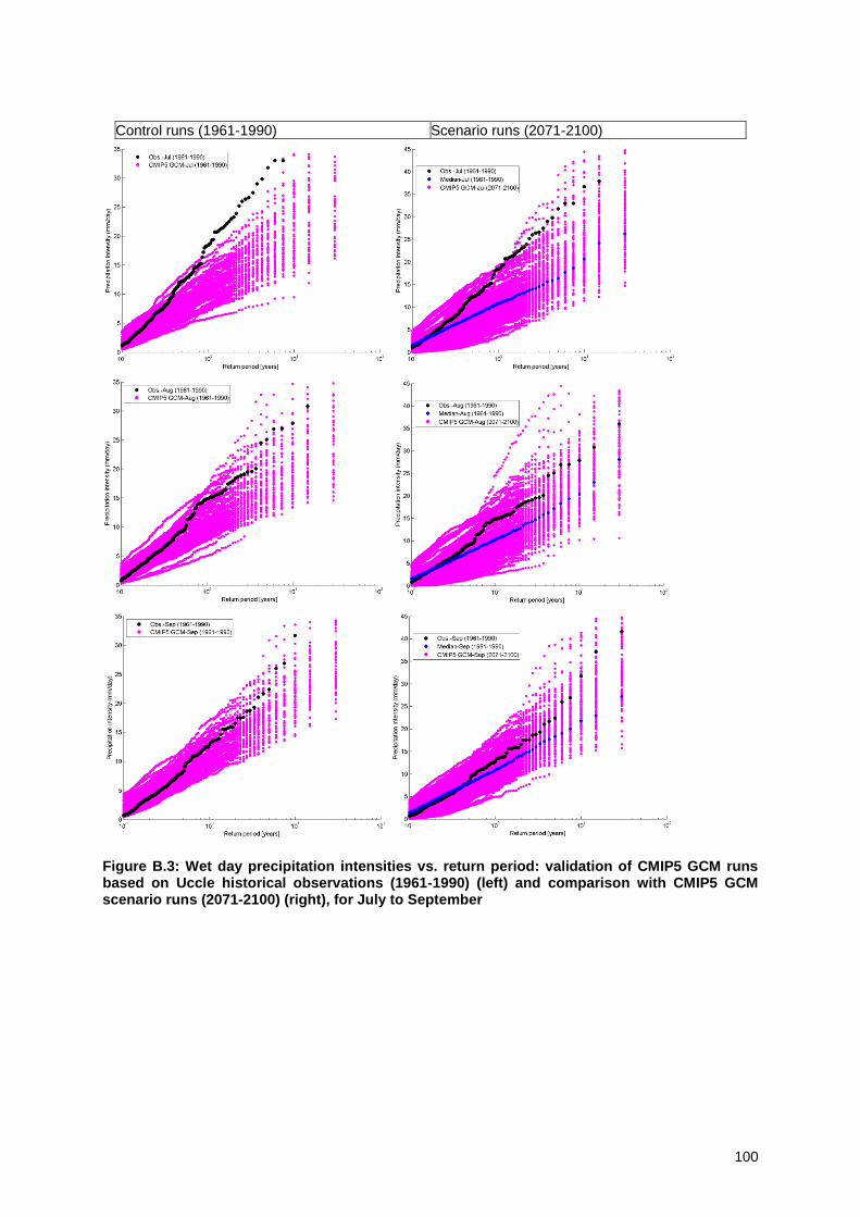
100

Control runs (1961-1990) Scenario runs (2071-2100)

Figure B.3: Wet day precipitation intensities vs. return period: validation of CMIP5 GCM runs based on Uccle historical observations (1961-1990) (left) and comparison with CMIP5 GCM scenario runs (2071-2100) (right), for July to September

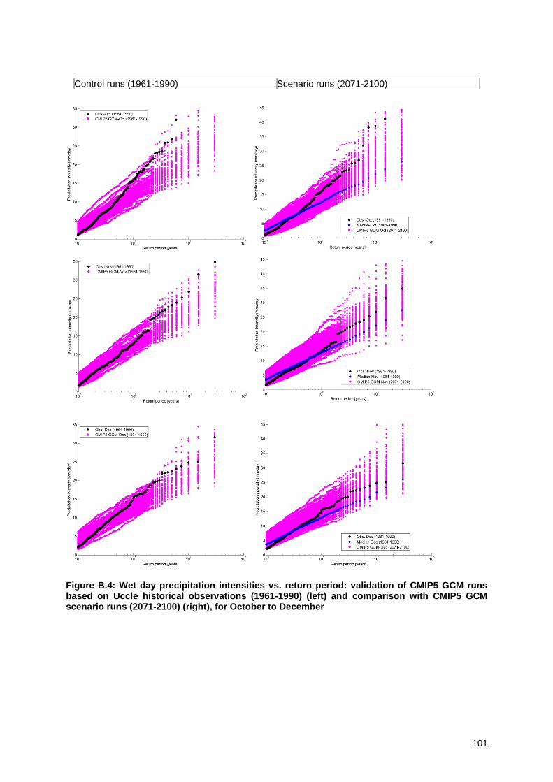
101



Figure B.4: Wet day precipitation intensities vs. return period: validation of CMIP5 GCM runs based on Uccle historical observations (1961-1990) (left) and comparison with CMIP5 GCM scenario runs (2071-2100) (right), for October to December

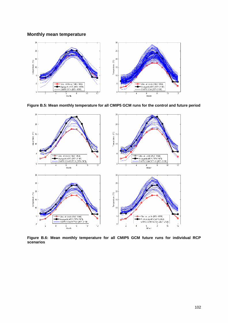
102

Monthly mean temperature

Figure B.5: Mean monthly temperature for all CMIP5 GCM runs for the control and future period

Figure B.6: Mean monthly temperature for all CMIP5 GCM future runs for individual RCP scenarios

103

Daily temperature quantiles: per season

Figure B.7: Temperature vs. return period: comparison of control and scenario period runs for winter (top) and summer (bottom) seasons

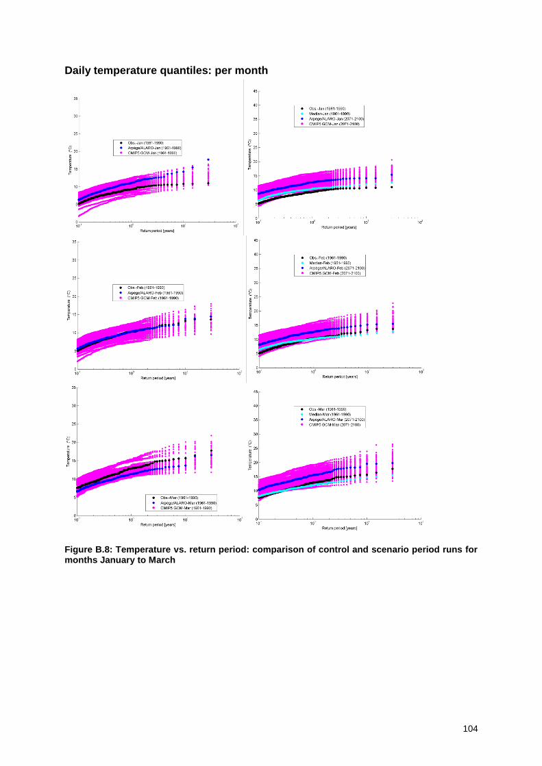
104

Daily temperature quantiles: per month

Figure B.8: Temperature vs. return period: comparison of control and scenario period runs for months January to March

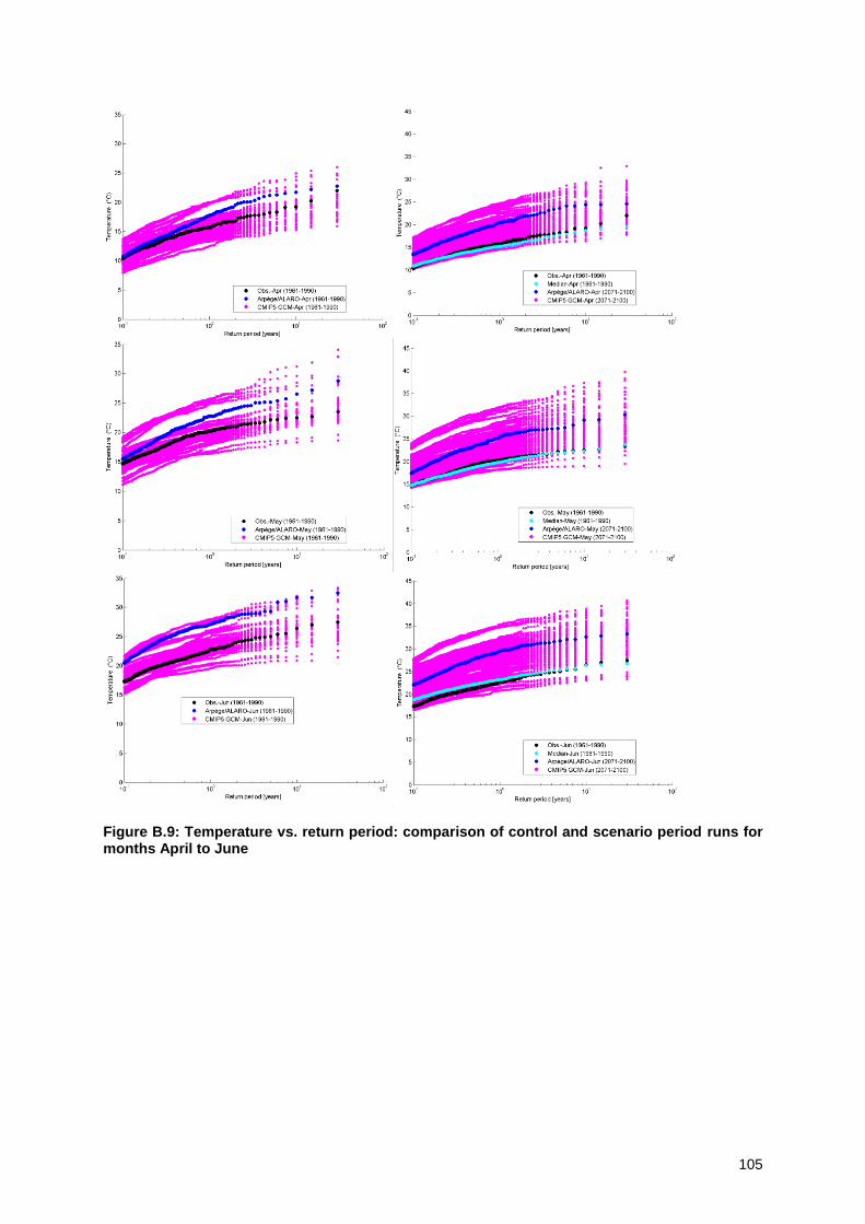
105

Figure B.9: Temperature vs. return period: comparison of control and scenario period runs for months April to June

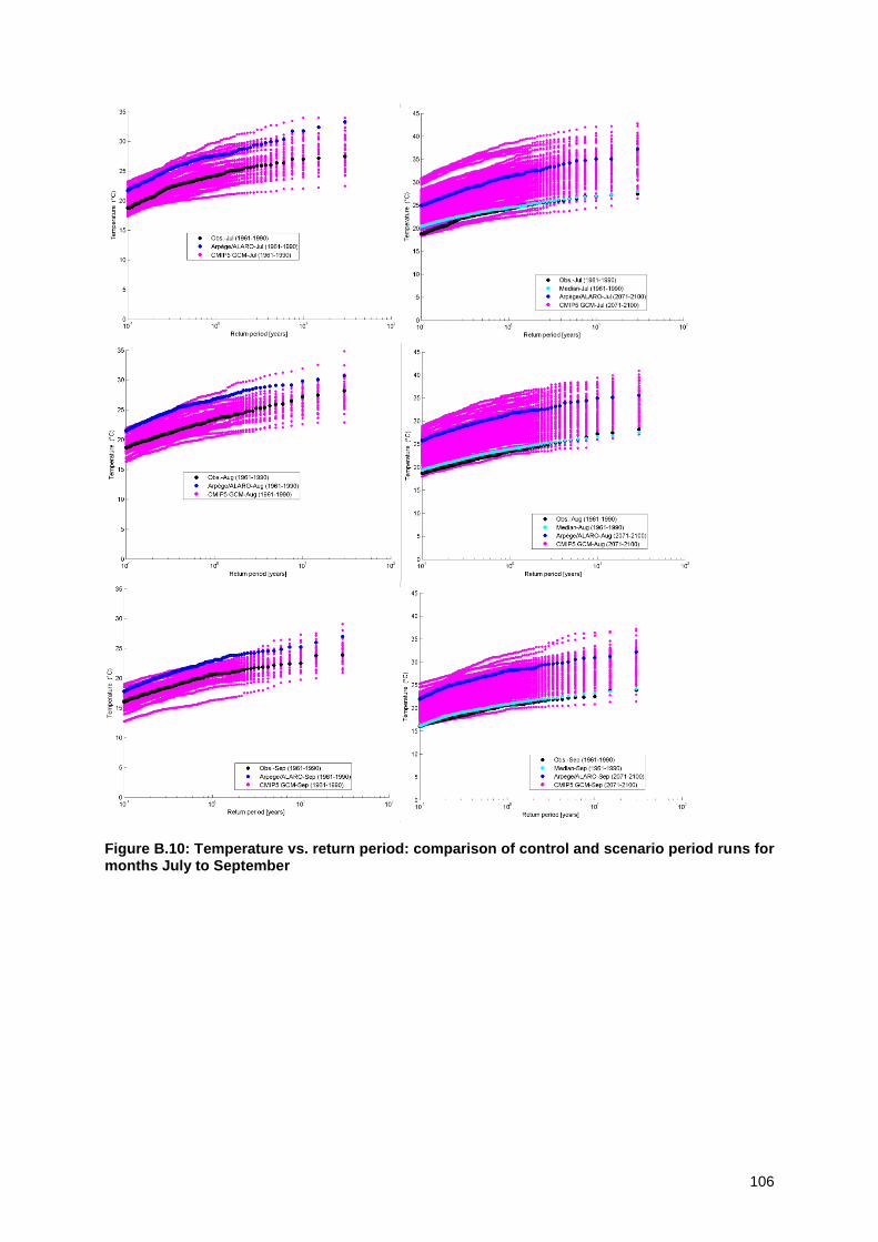
106

Figure B.10: Temperature vs. return period: comparison of control and scenario period runs for months July to September

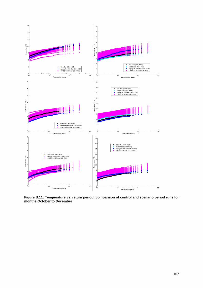
107

Figure B.11: Temperature vs. return period: comparison of control and scenario period runs for months October to December

Actualisatie en verfijning voor Vlaanderen · Koning Albert-II laan 20 1000 Brussel ... 6...

Documents

Transcript of Actualisatie en verfijning voor Vlaanderen · Koning Albert-II laan 20 1000 Brussel ... 6...