Pharmacometrics Research GroupDepartment of Pharmaceutical Biosciences

Uppsala UniversitySweden

A strategy for residual error modeling incorporating both scedasticity of variance and

distribution shape

Anne-Gaëlle Dosne, Ron J. Keizer, Martin Bergstrand, Mats O. Karlsson

2

Predictions

Res

idua

ls

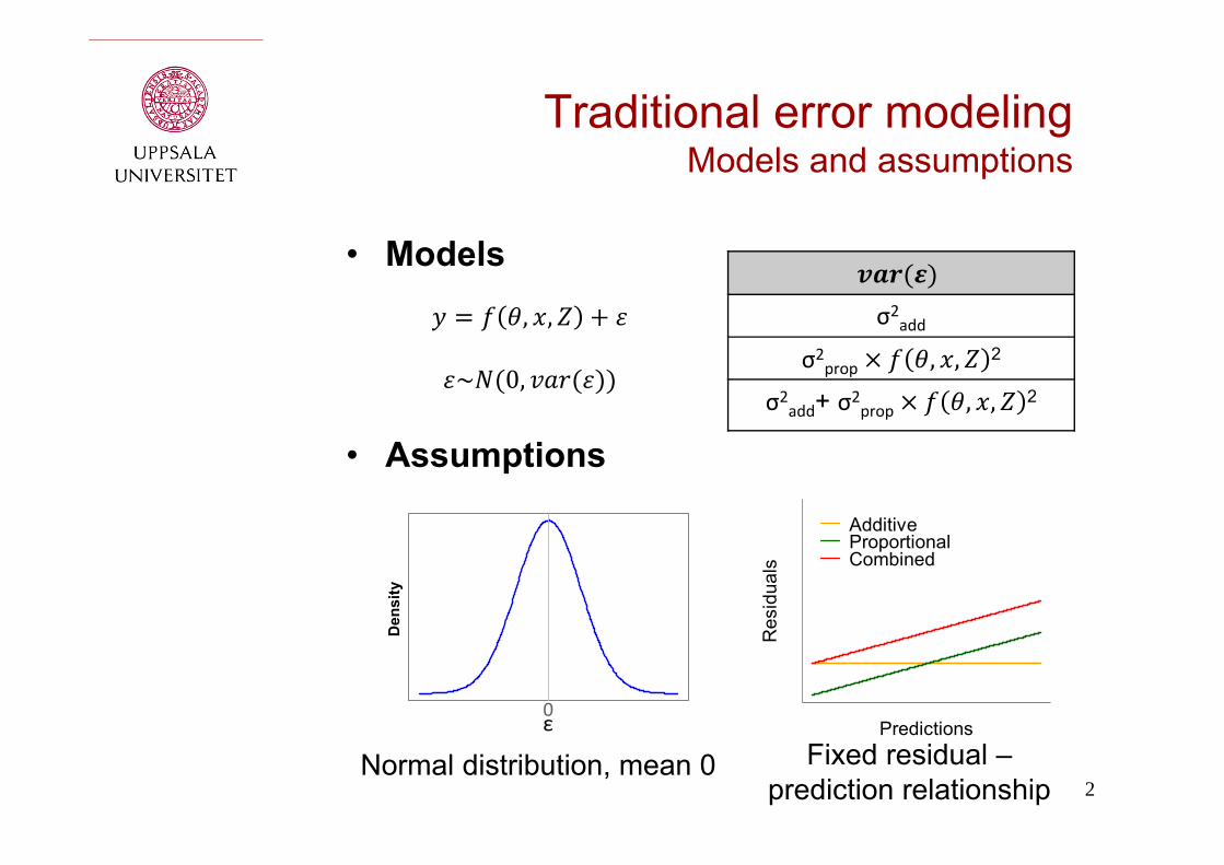
AdditiveProportionalCombined

, ,

~ 0,

σ2addσ2prop , , 2

σ2add+ σ2prop , , 2

Traditional error modelingModels and assumptions

Normal distribution, mean 0 Fixed residual –prediction relationship

Den

sity

0ε

• Models

• Assumptions

3

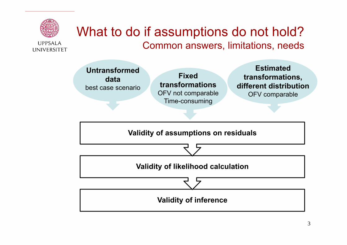
What to do if assumptions do not hold?Common answers, limitations, needs

Validity of inference

Validity of likelihood calculation

Validity of assumptions on residuals

Fixed transformations

OFV not comparableTime-consuming

Untransformed data

best case scenario

Estimated transformations,

different distribution OFV comparable

4

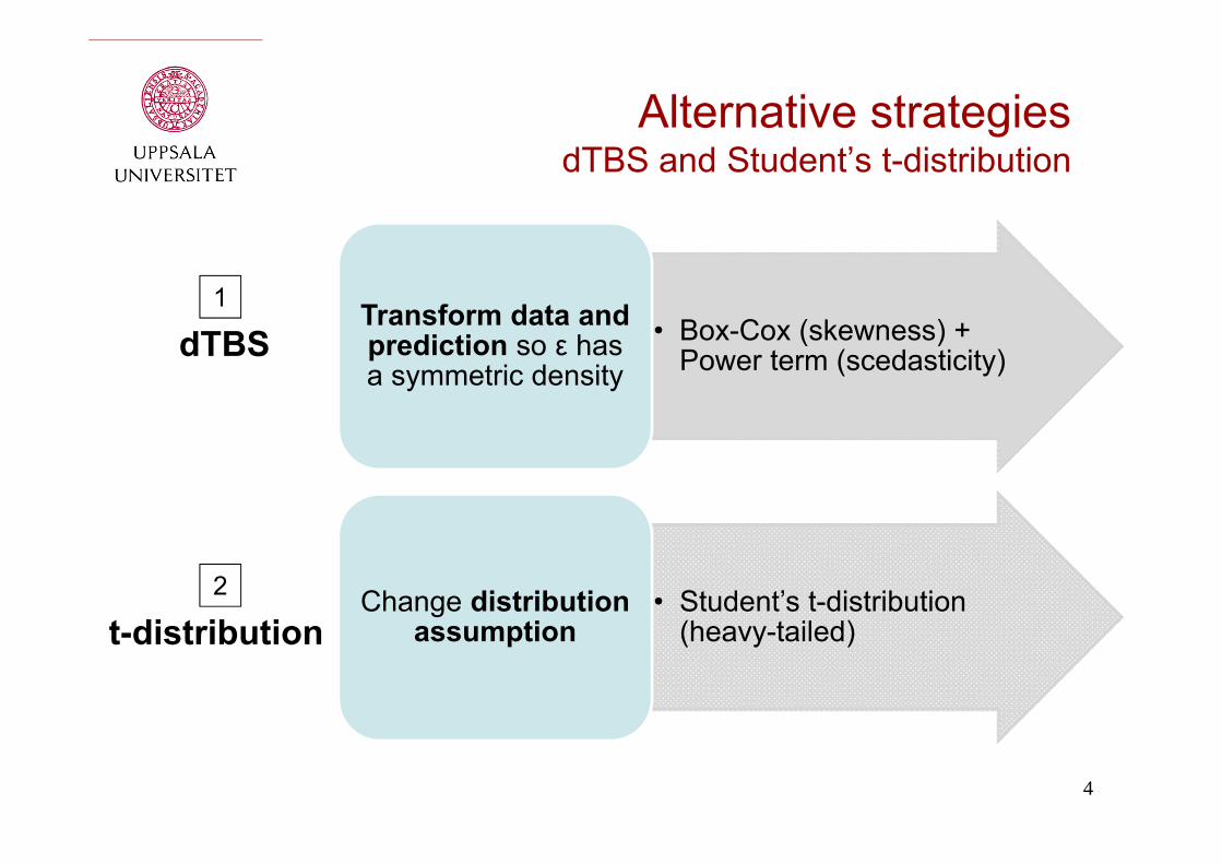
Alternative strategiesdTBS and Student’s t-distribution

• Box-Cox (skewness) + Power term (scedasticity)

Transform data and prediction so ε has a symmetric density

• Student’s t-distribution (heavy-tailed)

Change distribution assumption

dTBS

t-distribution

1

2

Residual error modeling with dynamic Transform Both

Sides (dTBS)

5

6

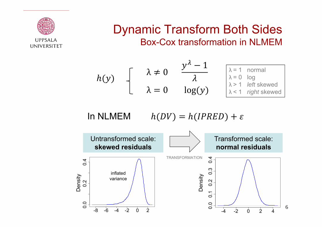
Dynamic Transform Both Sides Box-Cox transformation in NLMEM

λ 01

λ 0log

In NLMEM

-4 -2 0 2 40.

00.

10.

20.

30.

4

Untransformed scale:skewed residuals

Transformed scale:normal residuals

Den

sity

TRANSFORMATION

-8 -6 -4 -2 0 2

0.0

0.2

0.4

Den

sity inflated

variance

λ = 1 normalλ = 0 logλ > 1 left skewedλ < 1 right skewed

7

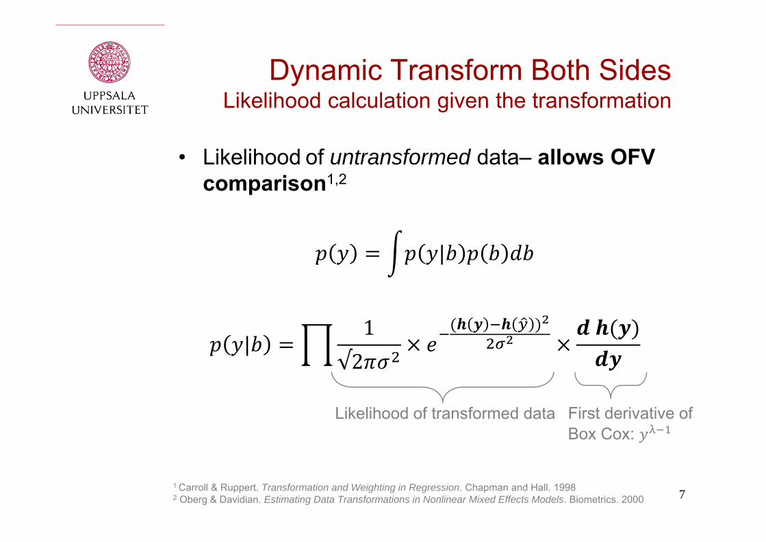
Dynamic Transform Both Sides Likelihood calculation given the transformation

• Likelihood of untransformed data– allows OFV comparison1,2

|

|1

√2

Likelihood of transformed data First derivative of Box Cox:

1 Carroll & Ruppert. Transformation and Weighting in Regression. Chapman and Hall. 19982 Oberg & Davidian. Estimating Data Transformations in Nonlinear Mixed Effects Models. Biometrics. 2000

8

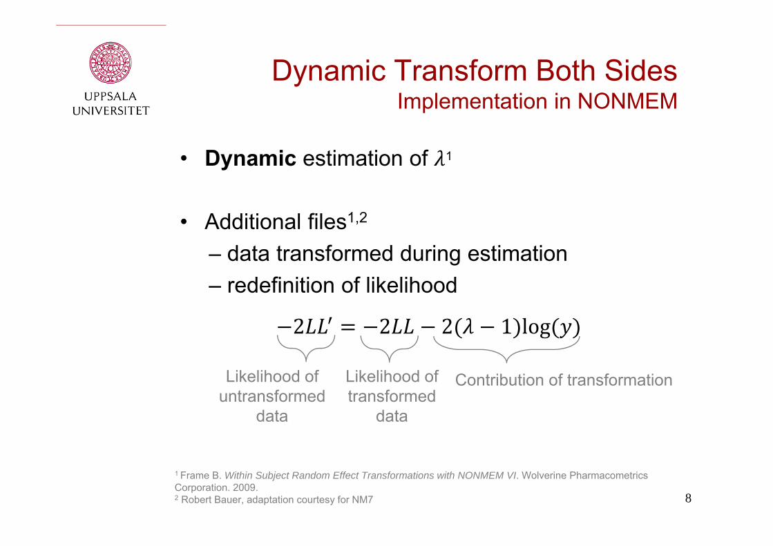
Dynamic Transform Both Sides Implementation in NONMEM

• Dynamic estimation of 1

• Additional files1,2

– data transformed during estimation– redefinition of likelihood

2 2 2 1 log

1 Frame B. Within Subject Random Effect Transformations with NONMEM VI. Wolverine Pharmacometrics Corporation. 2009.2 Robert Bauer, adaptation courtesy for NM7

Likelihood of untransformed

data

Likelihood of transformed

data

Contribution of transformation

9

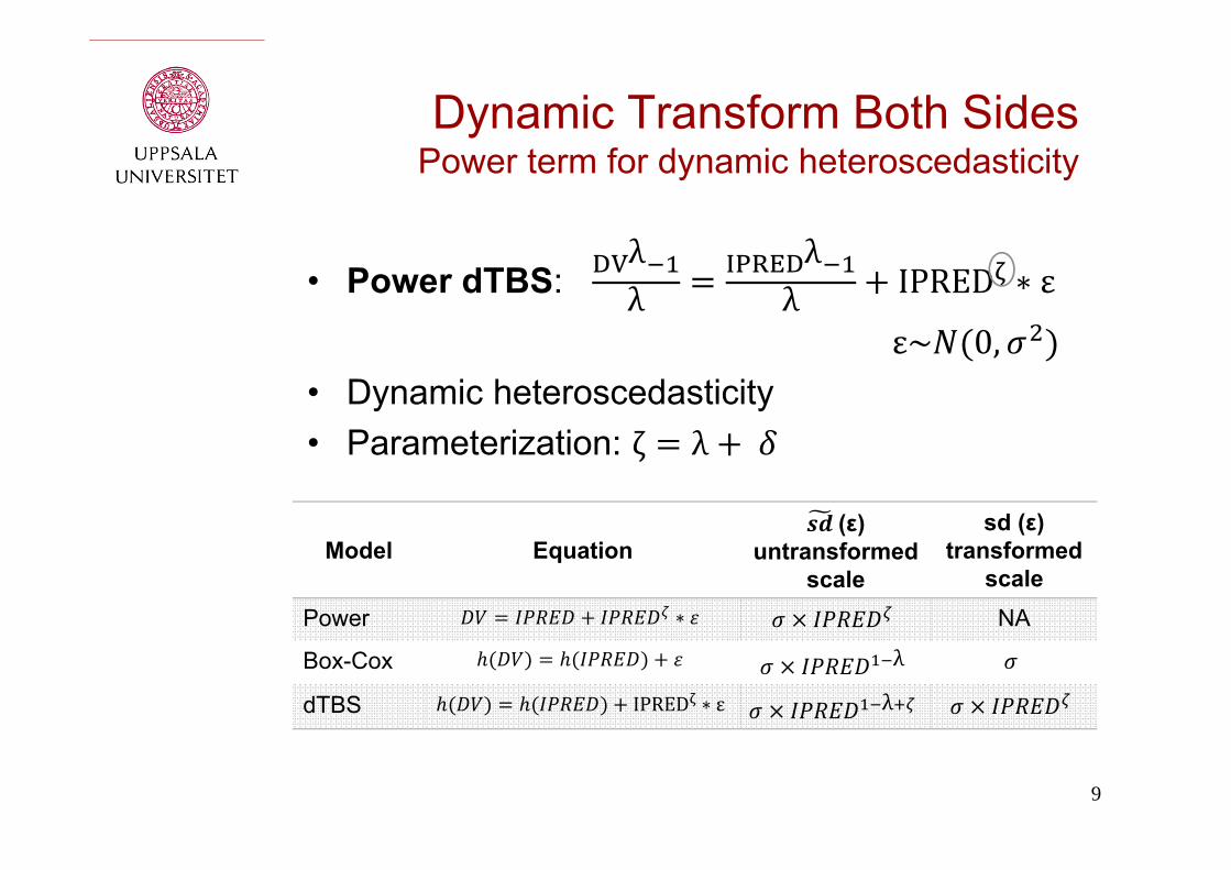
Dynamic Transform Both Sides Power term for dynamic heteroscedasticity

• Power dTBS: λλ

λλ IPRED ∗ ε

ε~ 0,• Dynamic heteroscedasticity• Parameterization: ζ λ

Model Equation(ε)

untransformed scale

sd (ε) transformed

scalePower ∗ NA

Box-Cox λ

dTBS IPRED ∗ ε λ

10

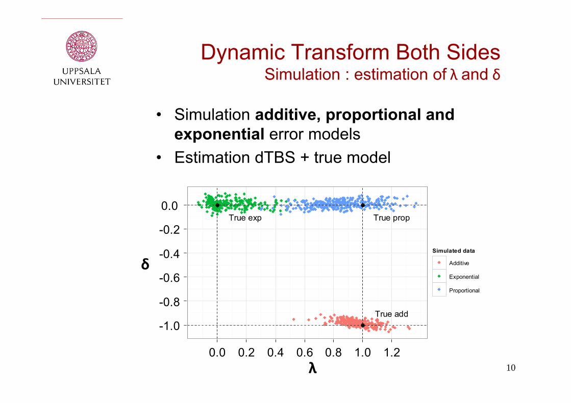
Dynamic Transform Both Sides Simulation : estimation of λ and δ

• Simulation additive, proportional and exponential error models

• Estimation dTBS + true model

-1.0

-0.8

-0.6

-0.4

-0.2

0.0

True add

True propTrue exp

0.0 0.2 0.4 0.6 0.8 1.0 1.2

Simulated data

Additive

Exponential

Proportional

δ

λ

11

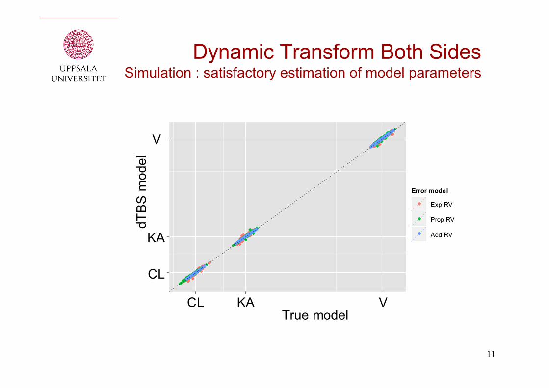
Dynamic Transform Both Sides Simulation : satisfactory estimation of model parameters

True model

dTB

S m

odel

CL

KA

V

CL KA V

Error model

Exp RV

Prop RV

Add RV

12

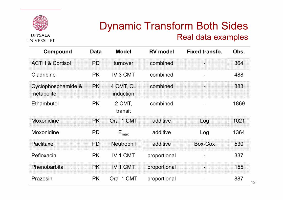
Dynamic Transform Both SidesReal data examples

Compound Data Model RV model Fixed transfo. Obs.

ACTH & Cortisol PD turnover combined - 364

Cladribine PK IV 3 CMT combined - 488

Cyclophosphamide & metabolite

PK 4 CMT, CLinduction

combined - 383

Ethambutol PK 2 CMT, transit

combined - 1869

Moxonidine PK Oral 1 CMT additive Log 1021

Moxonidine PD Emax additive Log 1364

Paclitaxel PD Neutrophil additive Box-Cox 530

Pefloxacin PK IV 1 CMT proportional - 337

Phenobarbital PK IV 1 CMT proportional - 155

Prazosin PK Oral 1 CMT proportional - 887

13

-250

-200

-150

-100

-50

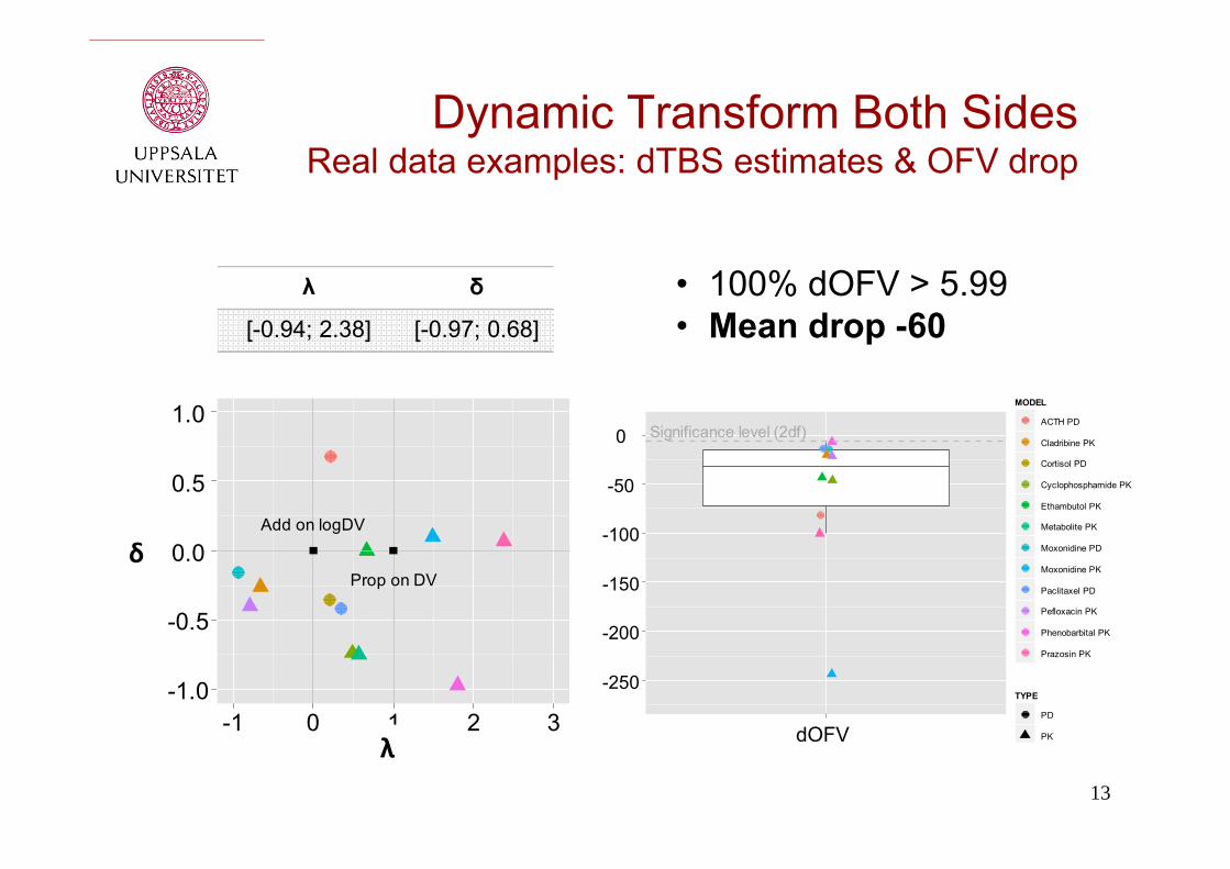
0 Significance level (2df)

MODEL

ACTH PD

Cladribine PK

Cortisol PD

Cyclophosphamide PK

Ethambutol PK

Metabolite PK

Moxonidine PD

Moxonidine PK

Paclitaxel PD

Pefloxacin PK

Phenobarbital PK

Prazosin PK

TYPE

PD

PK

Dynamic Transform Both SidesReal data examples: dTBS estimates & OFV drop

λ δ

[-0.94; 2.38] [-0.97; 0.68]

• 100% dOFV > 5.99• Mean drop -60

dOFV

-1.0

-0.5

0.0

0.5

1.0

Add on logDV

Prop on DV

-1 0 1 2 3

δ

λ

14

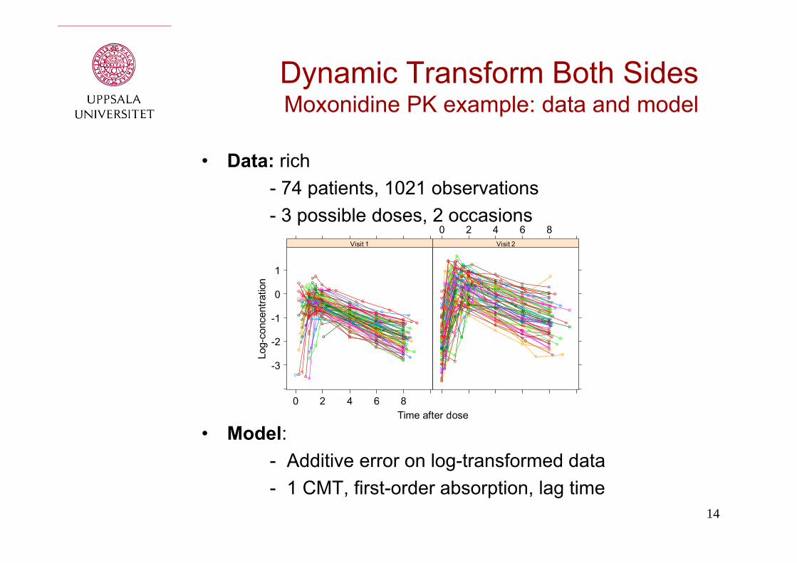
Dynamic Transform Both SidesMoxonidine PK example: data and model

• Data: rich- 74 patients, 1021 observations- 3 possible doses, 2 occasions

• Model:- Additive error on log-transformed data- 1 CMT, first-order absorption, lag time

Time after dose

Log-

conc

entra

tion

-3

-2

-1

0

1

0 2 4 6 8

Visit 1

0 2 4 6 8Visit 2

15

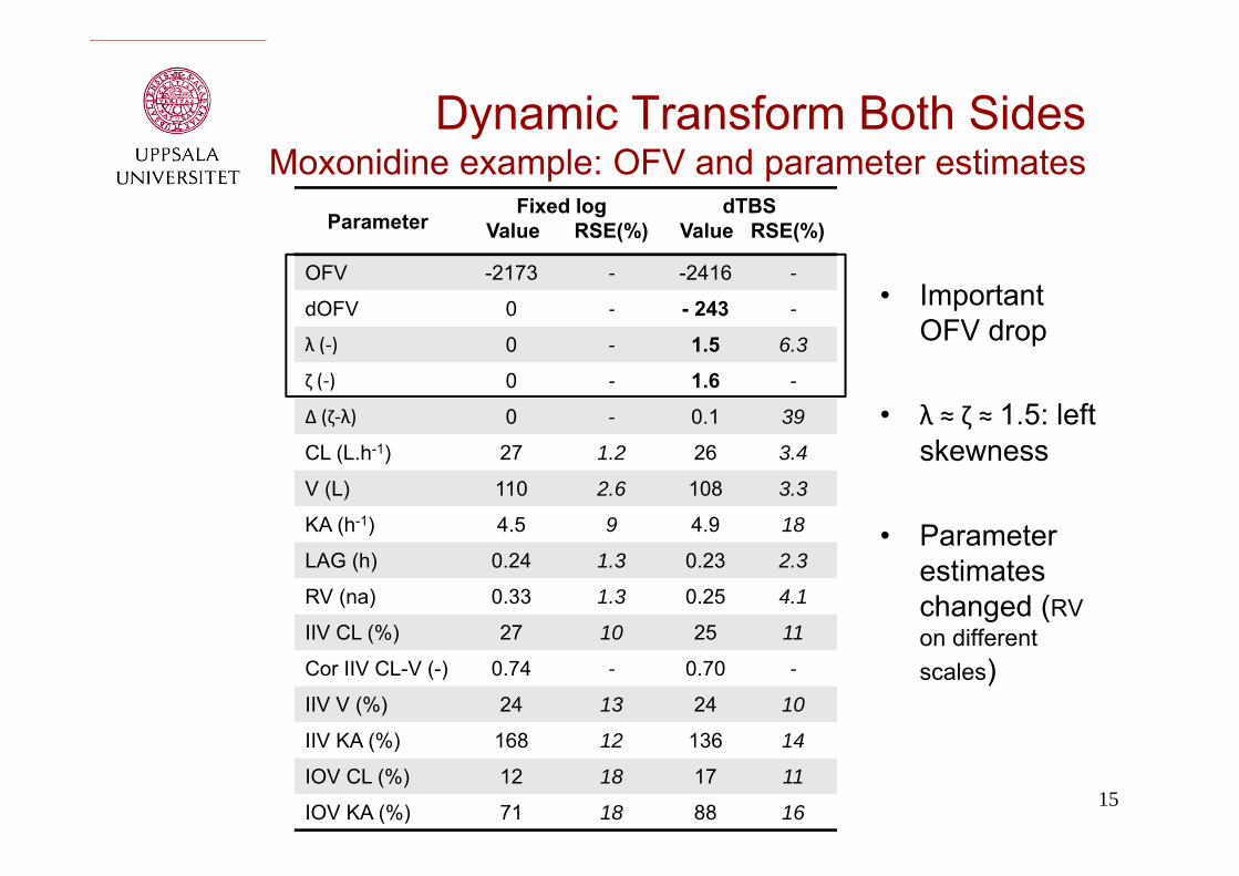
Dynamic Transform Both SidesMoxonidine example: OFV and parameter estimates

• Important OFV drop

• λ ≈ ζ ≈ 1.5: left skewness

• Parameter estimates changed (RV on different scales)

ParameterFixed log

Value RSE(%)dTBS

Value RSE(%)

OFV -2173 - -2416 -

dOFV 0 - - 243 -

λ (‐) 0 - 1.5 6.3

ζ (‐) 0 - 1.6 -

Δ (ζ‐λ) 0 - 0.1 39

CL (L.h-1) 27 1.2 26 3.4

V (L) 110 2.6 108 3.3

KA (h-1) 4.5 9 4.9 18

LAG (h) 0.24 1.3 0.23 2.3

RV (na) 0.33 1.3 0.25 4.1

IIV CL (%) 27 10 25 11

Cor IIV CL-V (-) 0.74 - 0.70 -

IIV V (%) 24 13 24 10

IIV KA (%) 168 12 136 14

IOV CL (%) 12 18 17 11

IOV KA (%) 71 18 88 16

16

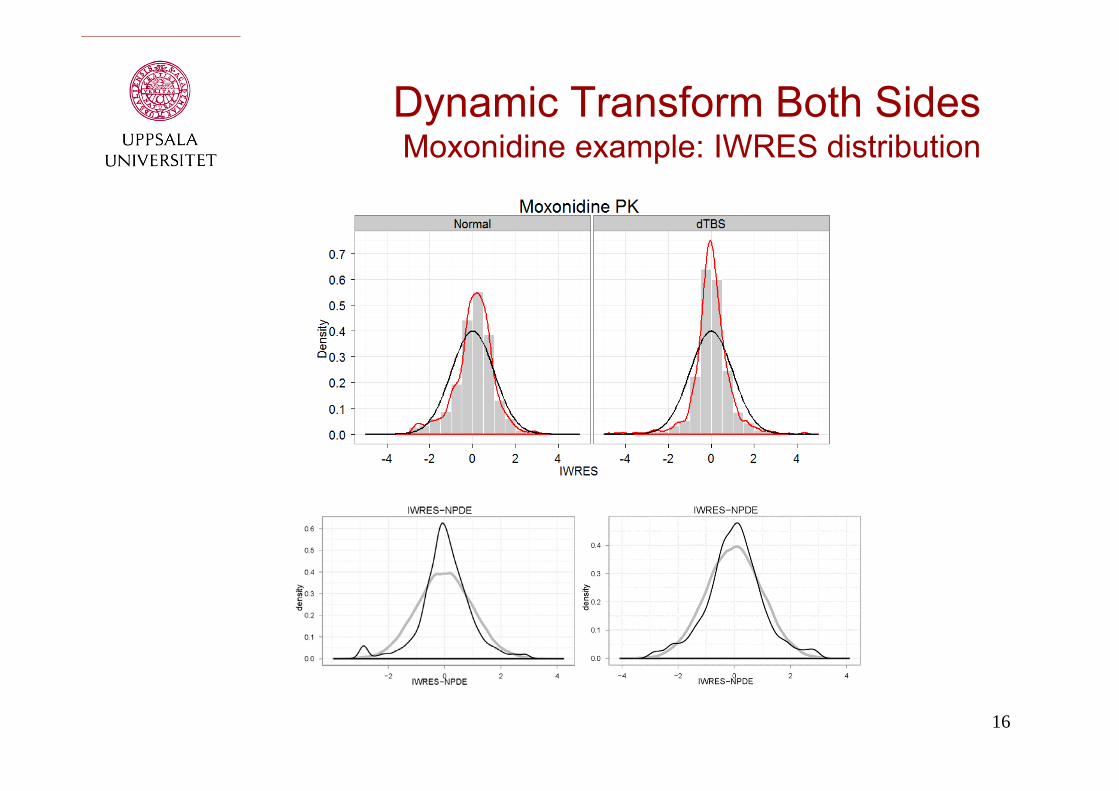
Dynamic Transform Both SidesMoxonidine example: IWRES distribution

17

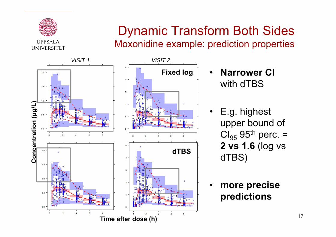
Dynamic Transform Both SidesMoxonidine example: prediction properties

• Narrower CI with dTBS

• E.g. highest upper bound of CI95 95th perc. = 2 vs 1.6 (log vsdTBS)

• more precise predictions

Time after dose (h)

VISIT 1 VISIT 2

Con

cent

ratio

n (μ

g/L)

dTBS

Fixed log

Residual error modeling with Student’s t-distribution

18

19

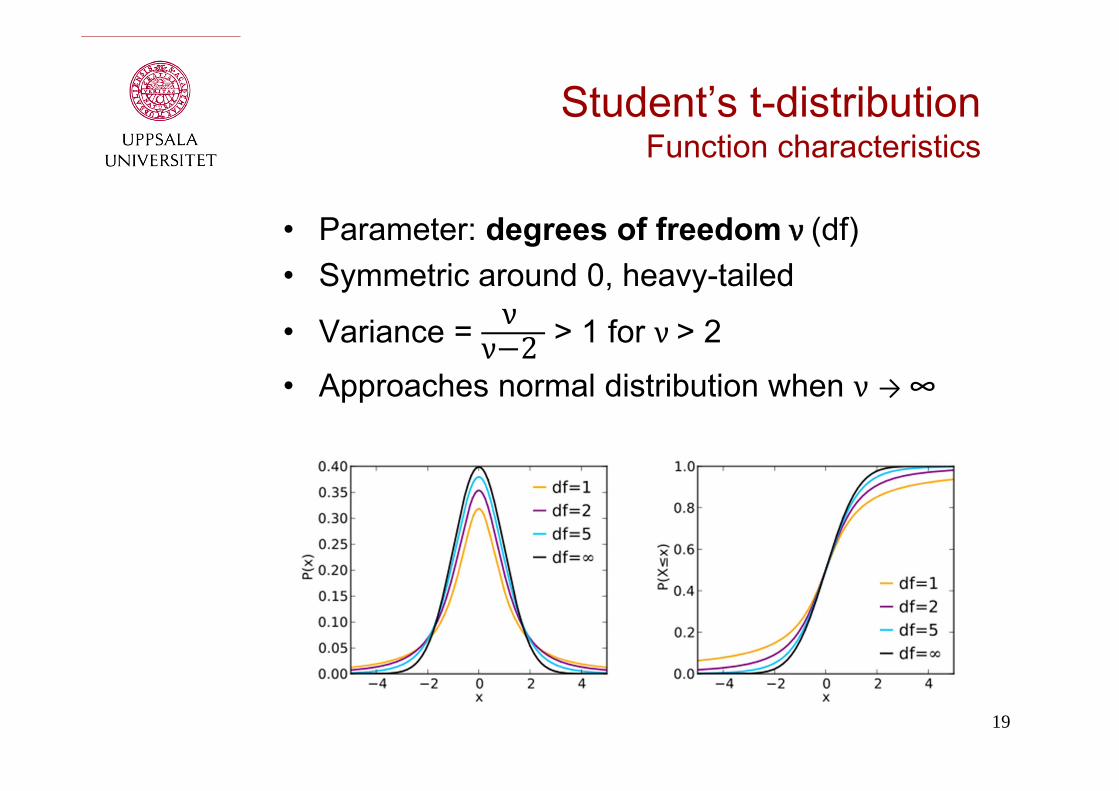
Student’s t-distributionFunction characteristics

• Parameter: degrees of freedom ν (df)• Symmetric around 0, heavy-tailed

• Variance = νν 2 > 1 for ν> 2

• Approaches normal distribution when ν → ∞

20

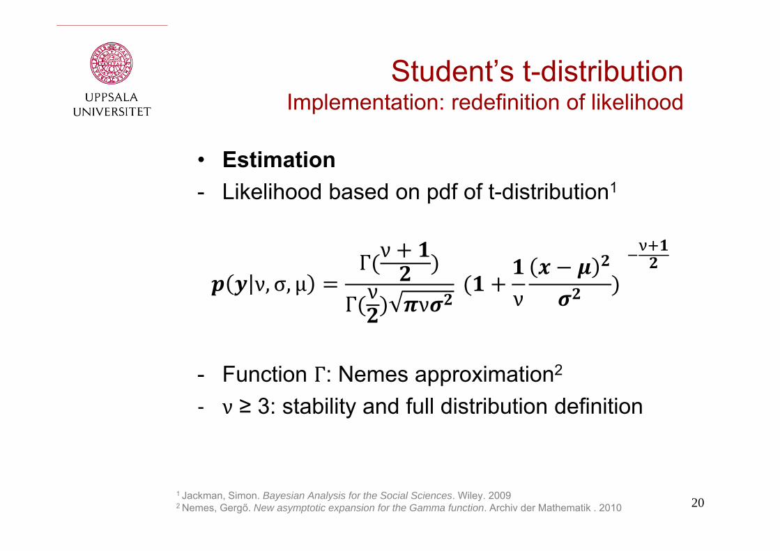
Student’s t-distributionImplementation: redefinition of likelihood

• Estimation- Likelihood based on pdf of t-distribution1

ν, σ, μΓ ν

Γ ν ν ν

- Function Γ: Nemes approximation2

‐ ν ≥ 3: stability and full distribution definition

1 Jackman, Simon. Bayesian Analysis for the Social Sciences. Wiley. 20092 Nemes, Gergő. New asymptotic expansion for the Gamma function. Archiv der Mathematik . 2010

21

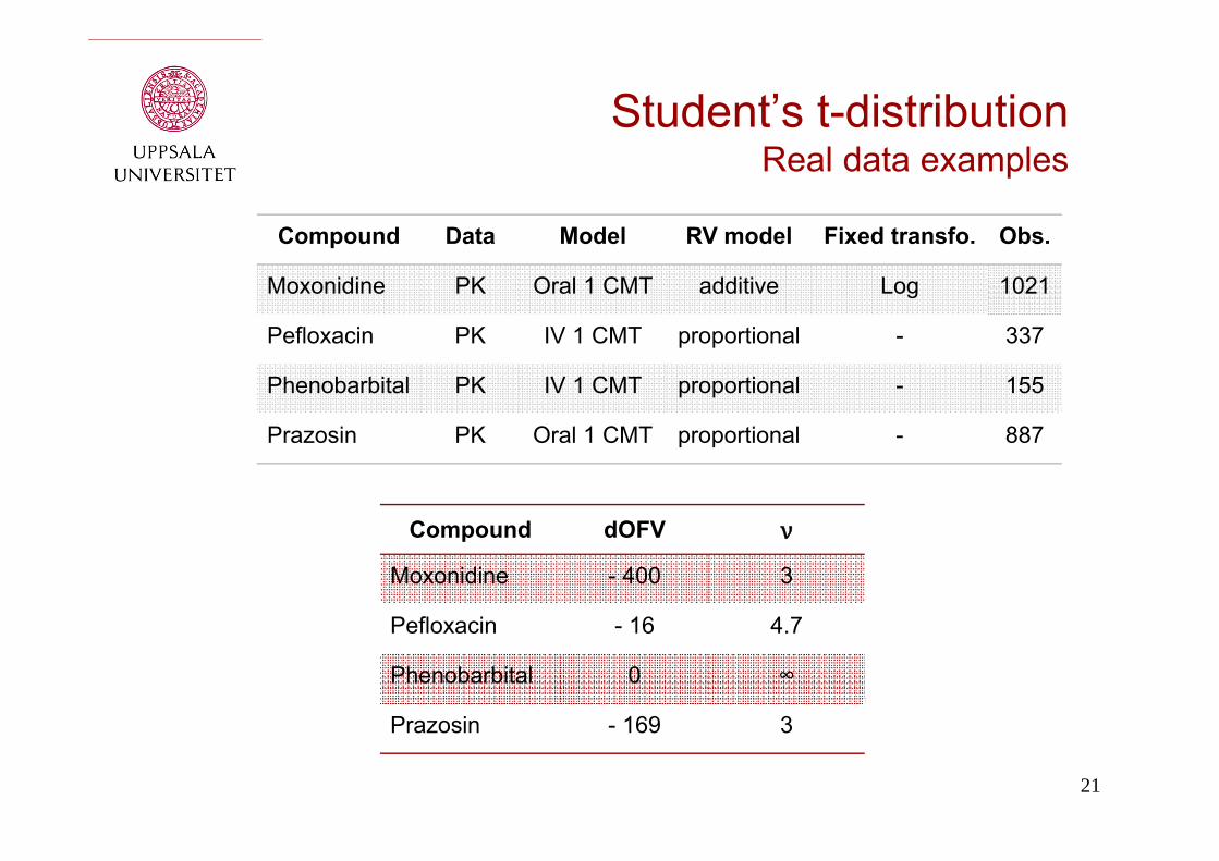
Student’s t-distributionReal data examples

Compound Data Model RV model Fixed transfo. Obs.

Moxonidine PK Oral 1 CMT additive Log 1021

Pefloxacin PK IV 1 CMT proportional - 337

Phenobarbital PK IV 1 CMT proportional - 155

Prazosin PK Oral 1 CMT proportional - 887

Compound dOFV ν

Moxonidine - 400 3

Pefloxacin - 16 4.7

Phenobarbital 0 ∞

Prazosin - 169 3

22

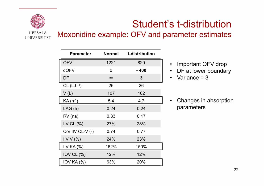
Student’s t-distributionMoxonidine example: OFV and parameter estimates

Parameter Normal t-distribution

OFV 1221 820

dOFV 0 - 400

DF ∞ 3

CL (L.h-1) 26 26

V (L) 107 102

KA (h-1) 5.4 4.7

LAG (h) 0.24 0.24

RV (na) 0.33 0.17

IIV CL (%) 27% 28%

Cor IIV CL-V (-) 0.74 0.77

IIV V (%) 24% 23%

IIV KA (%) 162% 150%

IOV CL (%) 12% 12%

IOV KA (%) 63% 20%

• Important OFV drop• DF at lower boundary• Variance = 3

• Changes in absorption parameters

23

IWRES

Den

sity

0.0

0.2

0.4

0.6

0.8

-10 -5 0 5 10IWRES

Den

sity

0.0

0.2

0.4

0.6

0.8

-10 -5 0 5 10

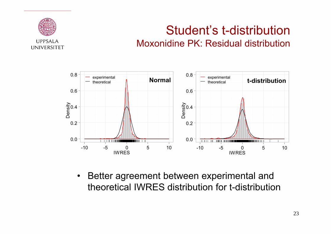
Student’s t-distributionMoxonidine PK: Residual distribution

• Better agreement between experimental and theoretical IWRES distribution for t-distribution

Normal t-distributionexperimental theoretical

experimental theoretical

24

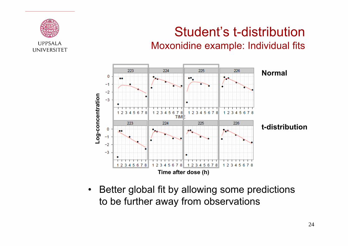
Student’s t-distribution Moxonidine example: Individual fits

Normal

• Better global fit by allowing some predictions to be further away from observations

t-distribution

Log-

conc

entr

atio

n

Time after dose (h)

25

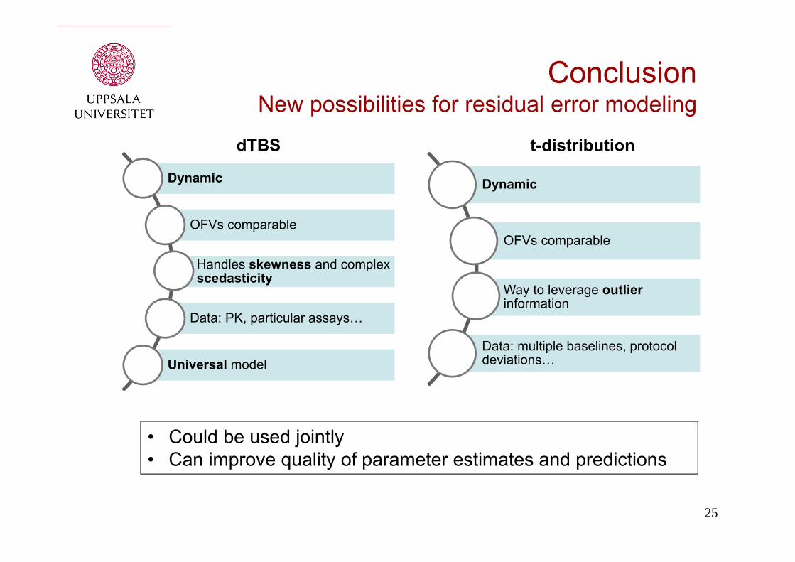
ConclusionNew possibilities for residual error modeling

Dynamic

OFVs comparable

Way to leverage outlierinformation

Data: multiple baselines, protocol deviations…

Dynamic

OFVs comparable

Handles skewness and complex scedasticity

Data: PK, particular assays…

Universal model

• Could be used jointly• Can improve quality of parameter estimates and predictions

dTBS t-distribution

26

AcknowledgementsThe research leading to these results has received support from the Innovative Medicines Initiative Joint Undertaking under grant agreement n° 115156, resources of which are composed of financial contributions from the European Union's Seventh Framework Programme (FP7/2007-2013) and EFPIA companies’ in kind contribution. The DDMoRe project is also supported by financial contribution from Academic and SME partners. This work does not necessarily represent the view of all DDMoRepartners.

• Uppsala Pharmacometrics Research Group

• Novartis for financial support

27

Additional slides

• dTBS ccontra and contr files• dTBS model file code• dTBS simulation code • t-distribution simulation code • Type I error investigation for dTBS and t-

distribution

28

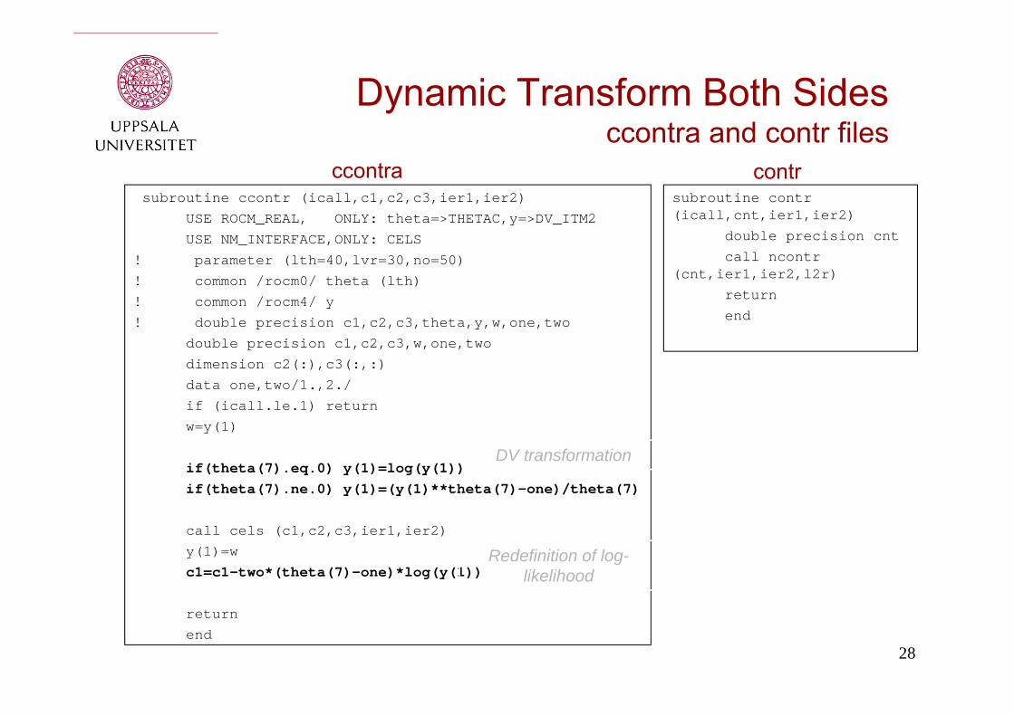
Dynamic Transform Both Sides ccontra and contr files

subroutine ccontr (icall,c1,c2,c3,ier1,ier2)USE ROCM_REAL, ONLY: theta=>THETAC,y=>DV_ITM2USE NM_INTERFACE,ONLY: CELS

! parameter (lth=40,lvr=30,no=50)! common /rocm0/ theta (lth)! common /rocm4/ y! double precision c1,c2,c3,theta,y,w,one,two

double precision c1,c2,c3,w,one,twodimension c2(:),c3(:,:)data one,two/1.,2./if (icall.le.1) returnw=y(1)

if(theta(7).eq.0) y(1)=log(y(1))if(theta(7).ne.0) y(1)=(y(1)**theta(7)-one)/theta(7)

call cels (c1,c2,c3,ier1,ier2)y(1)=wc1=c1-two*(theta(7)-one)*log(y(1))

returnend

subroutine contr (icall,cnt,ier1,ier2)

double precision cntcall ncontr

(cnt,ier1,ier2,l2r)returnend

DV transformation

Redefinition of log-likelihood

ccontra contr

29

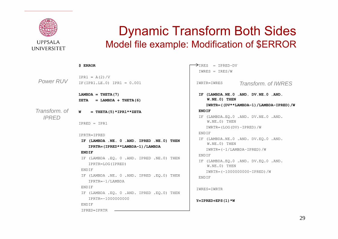
Dynamic Transform Both Sides Model file example: Modification of $ERROR

$ ERROR

IPR1 = A(2)/VIF(IPR1.LE.0) IPR1 = 0.001

LAMBDA = THETA(7)ZETA = LAMBDA + THETA(6)

W = THETA(5)*IPR1**ZETA

IPRED = IPR1

IPRTR=IPREDIF (LAMBDA .NE. 0 .AND. IPRED .NE.0) THEN

IPRTR=(IPRED**LAMBDA-1)/LAMBDAENDIFIF (LAMBDA .EQ. 0 .AND. IPRED .NE.0) THEN

IPRTR=LOG(IPRED)ENDIFIF (LAMBDA .NE. 0 .AND. IPRED .EQ.0) THEN

IPRTR=-1/LAMBDAENDIFIF (LAMBDA .EQ. 0 .AND. IPRED .EQ.0) THEN

IPRTR=-1000000000ENDIFIPRED=IPRTR

IRES = IPRED-DVIWRES = IRES/W

IWRTR=IWRES

IF (LAMBDA.NE.0 .AND. DV.NE.0 .AND. W.NE.0) THENIWRTR=((DV**LAMBDA-1)/LAMBDA-IPRED)/W

ENDIFIF (LAMBDA.EQ.0 .AND. DV.NE.0 .AND.

W.NE.0) THENIWRTR=(LOG(DV)-IPRED)/W

ENDIFIF (LAMBDA.NE.0 .AND. DV.EQ.0 .AND.

W.NE.0) THENIWRTR=(-1/LAMBDA-IPRED)/W

ENDIFIF (LAMBDA.EQ.0 .AND. DV.EQ.0 .AND.

W.NE.0) THENIWRTR=(-1000000000-IPRED)/W

ENDIF

IWRES=IWRTR

Y=IPRED+EPS(1)*W

Power RUV

Transform. of IPRED

Transform. of IWRES

30

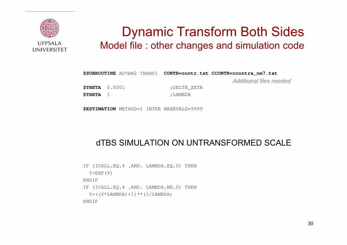
Dynamic Transform Both Sides Model file : other changes and simulation code

$SUBROUTINE ADVAN2 TRANS1 CONTR=contr.txt CCONTR=ccontra_nm7.txt

$THETA 0.0001 ;DELTA_ZETA$THETA 1 ;LAMBDA

$ESTIMATION METHOD=1 INTER MAXEVALS=9999

dTBS SIMULATION ON UNTRANSFORMED SCALE

IF (ICALL.EQ.4 .AND. LAMBDA.EQ.0) THENY=EXP(Y)

ENDIFIF (ICALL.EQ.4 .AND. LAMBDA.NE.0) THEN

Y=((Y*LAMBDA)+1)**(1/LAMBDA)ENDIF

Additional files needed

31

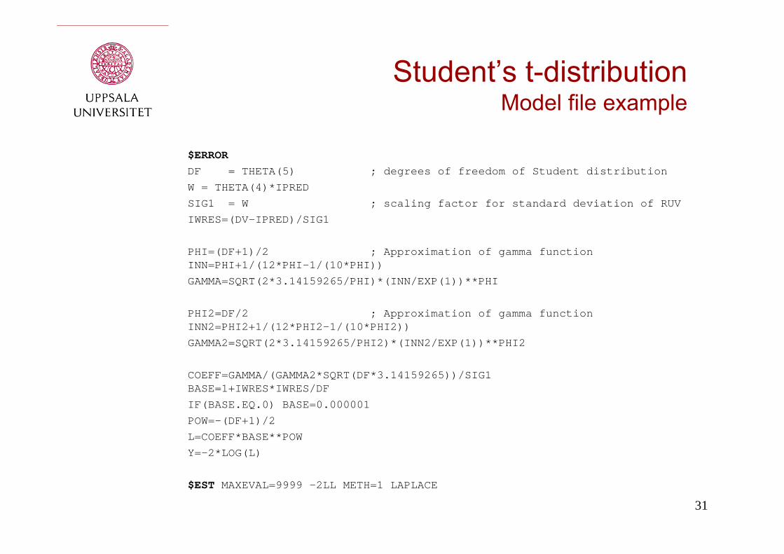
Student’s t-distributionModel file example

$ERRORDF = THETA(5) ; degrees of freedom of Student distributionW = THETA(4)*IPREDSIG1 = W ; scaling factor for standard deviation of RUVIWRES=(DV-IPRED)/SIG1

PHI=(DF+1)/2 ; Approximation of gamma function INN=PHI+1/(12*PHI-1/(10*PHI))GAMMA=SQRT(2*3.14159265/PHI)*(INN/EXP(1))**PHI

PHI2=DF/2 ; Approximation of gamma function INN2=PHI2+1/(12*PHI2-1/(10*PHI2))GAMMA2=SQRT(2*3.14159265/PHI2)*(INN2/EXP(1))**PHI2

COEFF=GAMMA/(GAMMA2*SQRT(DF*3.14159265))/SIG1 BASE=1+IWRES*IWRES/DF IF(BASE.EQ.0) BASE=0.000001POW=-(DF+1)/2L=COEFF*BASE**POWY=-2*LOG(L)

$EST MAXEVAL=9999 -2LL METH=1 LAPLACE

32

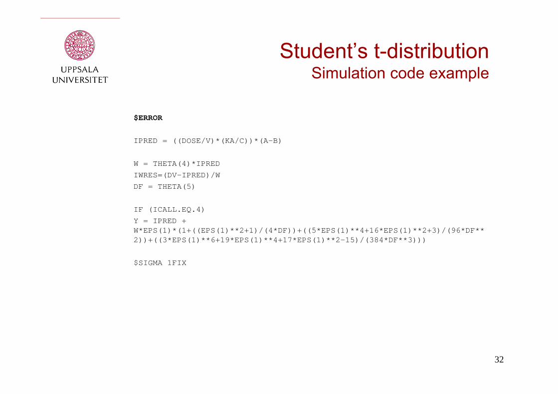
Student’s t-distributionSimulation code example

$ERROR

IPRED = ((DOSE/V)*(KA/C))*(A-B)

W = THETA(4)*IPREDIWRES=(DV-IPRED)/WDF = THETA(5)

IF (ICALL.EQ.4)Y = IPRED + W*EPS(1)*(1+((EPS(1)**2+1)/(4*DF))+((5*EPS(1)**4+16*EPS(1)**2+3)/(96*DF**2))+((3*EPS(1)**6+19*EPS(1)**4+17*EPS(1)**2-15)/(384*DF**3)))

$SIGMA 1FIX

33

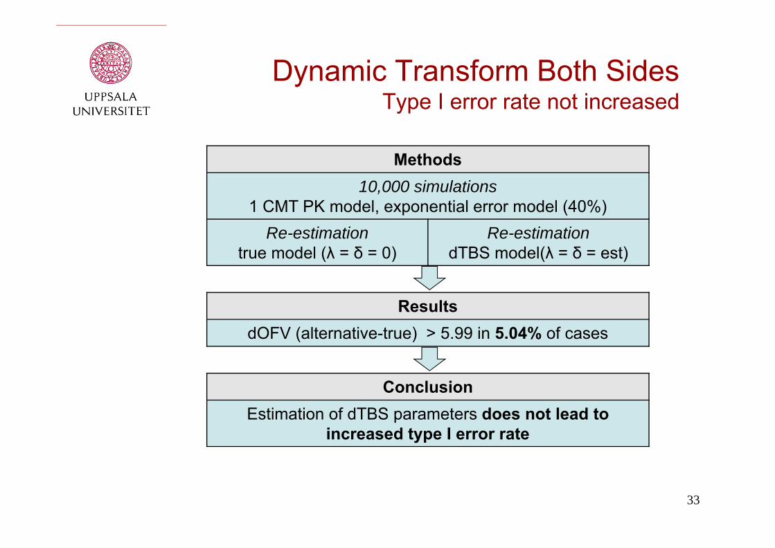
Dynamic Transform Both Sides Type I error rate not increased

Methods10,000 simulations

1 CMT PK model, exponential error model (40%)Re-estimation

true model (λ = δ = 0)Re-estimation

dTBS model(λ = δ = est)

ResultsdOFV (alternative-true) > 5.99 in 5.04% of cases

ConclusionEstimation of dTBS parameters does not lead to

increased type I error rate

34

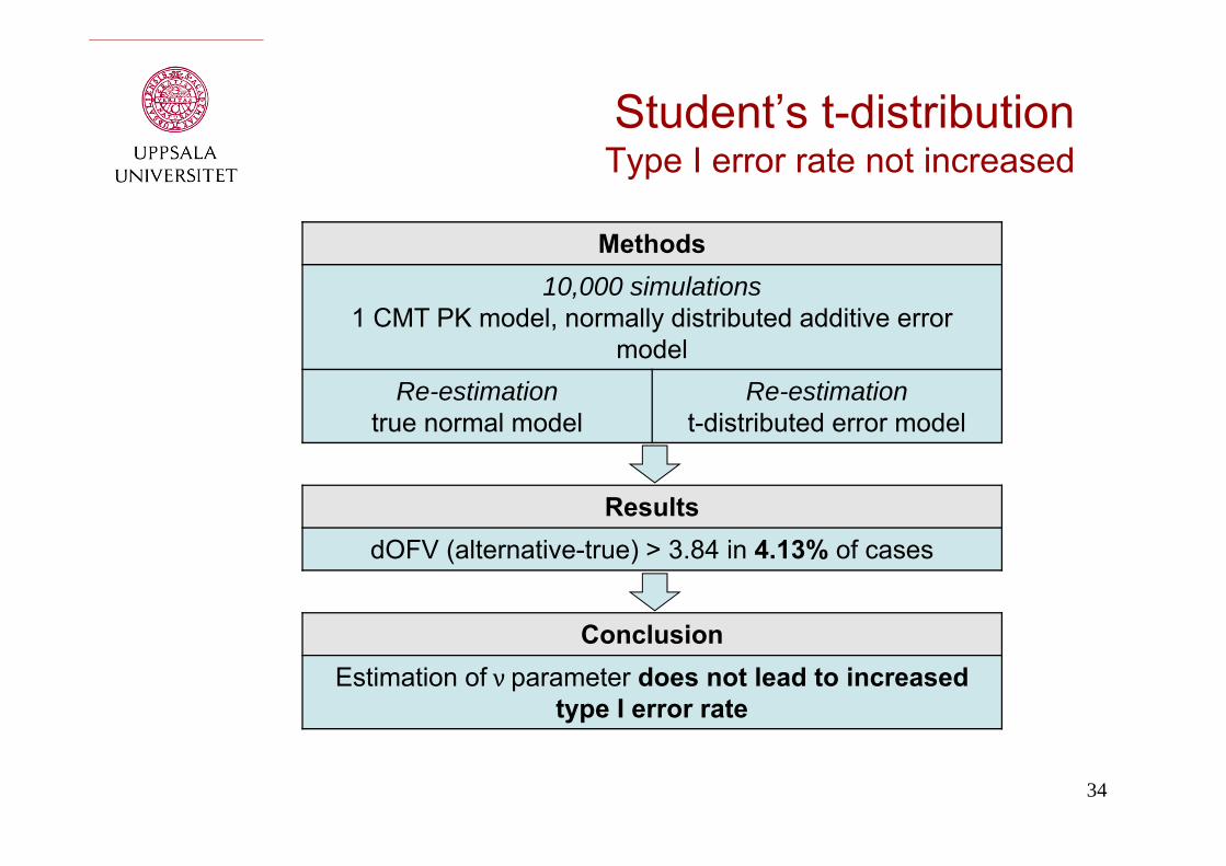
Student’s t-distributionType I error rate not increased

Methods10,000 simulations

1 CMT PK model, normally distributed additive error model

Re-estimationtrue normal model

Re-estimationt-distributed error model

ResultsdOFV (alternative-true) > 3.84 in 4.13% of cases

ConclusionEstimation of νparameter does not lead to increased

type I error rate