A REVIEW OF PARTIAL DIFFERENTIAL EQUATIONS OF THE FIRST

ORDER IN DYNAMICAL SYSTEMS

A MS.c Thesis

Presented by

Ahmed Abd Allah EL-KAHLOUT

Submitted in Partial Fulfillment of the

Requirements for MSc. Degree

in

MATHEMATICS

TO

Faculty of Science of

The Islamic University of Gaza

1998

ii

بسم اهللا الرحمن الرحيم

iii

إلىوالدي

وزوجتي

وابنتي نداء

ملخص البحث

iv

األنظمة في األولىمراجعة للمعادالت التفاضلیة الجزئیة من الدرجة المتحركة

رسالة ماجستیر مقدمة من الطالب

أحمد عبد اهللا الكحلوت ناصر فرحات.د: بإشراف

صفحة70 ،1998یولیو

وقد ناقشنا ،األولىلجزئیة من الدرجة ا التفاضلیة التفي ھد ا البحث قمنا بدراسة المعاد التوحل المعاد األولى الدرجة الجزئیة من التفاضلیة التالعالقة بین حل المعاد بالتفصیل المقیدة ھي معادالت تفاضلیة كاملة یمكن األنظمةمعادالت الحركة في .الكاملة التفاضلیة

المعادلة التفاضلیة الجزئیة ذلك قمنا بتكوین عالوة على. حققت شروط قابلیة التكاملإذاحلھا . من النظامین المنفصل والمتصل لكلبيوكاج-ھملتن

ABSTRACT

v

A REVIEW OF PARTIAL DIFFERENTIAL EQUATIONS OF THE FIRST

ORDER IN DYNAMICAL SYSTEMS

MSc. Thesis in Mathematics

By: Ahmed Abd Allah EL-KAHLOUT

Supervisor: Dr Nasser FARAHAT

July, 1998, 70 pages

The first order partial differential equations are studied in this thesis.The

relation between the solution of a system of first order partial differential equations

and a system of total differential equations and is discussed.

The investigation of singular system leads to total differential equations

which are integrable under certain integrability conditions. Furthermore; Hamilton-

Jacobi partial differential equation (HJPDE) is constructed in both discrete and

continuous systems.

ACKNOWLEDGMENTS

vi

I have the pleasure to express my thanks to my sincere supervisor

Dr. Nasser Farahat for his greet efforts to guide throughout this work. I am

also grateful to all my teachers in the Department of Mathematics at the

Islamic University-Gaza for providing me with rich ideas during my study.

Additional persons to whom I am indebted are Dr. Mohammed I.

Riffi, the Head of Dept. of Math., and Dr. Mohammed. M. Shabat for their

contribution in the supervision process as well as in defending this work.

Finally my deep thanks to my family who always encouraged me to

complete this thesis.

TABLE OF CONTENTS

iv ملخص البحث

ABSTRACT v

ACKNOWLEDGMENTS vi

CHAPTER I: INTRODUCTION

1

vii

CHAPTER II: INTEGRABILITY CONDITIONS OF SINGULAR SYSTEMS

5

2.1. The relations between the solutions of total differential

equations and (LHPDES).

5

2.2. Complete system of (LHPDES) of the first order

15

2.3. Integration of singular systems

18

CHAPTER III: HAMILTON-JACOBI PARTIAL DIFFERENTIAL

EQUATIONS FOR DISCRETE REGULAR CONSTRAINED SYSTEMS 29

3.1. Construction of (HJPDES) for discrete constrained

dynamical systems. 29

3.2. Integration of the (HJPDE) in discrete systems 36

CHAPTER IV: HAMILTON-JACOBI THEORY OF CONTENEOUS

SYSTEMS 42

4.1. Determination of the (HJPDE).for continuous systems 42

4.2. Integration of the (HJPDE) of continuous systems 48

CHAPTER V: CONCLUSION 68

1

CHAPTER I

INTRODUCTON

Any equation that contains differential coefficient is called a differential equation.

Such equations can be divide into two main types: ordinary and partial. Ordinary

differential equations involve only one independent variable, and partial differential

equations involve two or more independent variables. In general, any function of

x, y and the derivatives of y up to any order such that

F x yd yd x

d yd x

[ , , , ,......]2

2 0= (1.1)

defines an ordinary differential equation of y , where as the equations

F x y uux

uy

ux

uy

[ , ,..., , , ,..., , ,..]∂∂

∂∂

∂∂

∂∂

2

2

2

2 0= (1.2)

is partial differential equations for u (the dependent variable) in term of the

independent variables x, y,... .

The order of any differential equation is the order of the highest derivative

that appears in the equation. These equations are linear in the sense that both u and

its derivatives occur only to the first power, and the product of u and its

derivatives are absent, [1], [2].

In general, the solution of partial differential equations presents a much

more difficult problem than the solution of ordinary differential equations, and

except for certain special types of linear partial differential equations no general

method of solution is available.

2

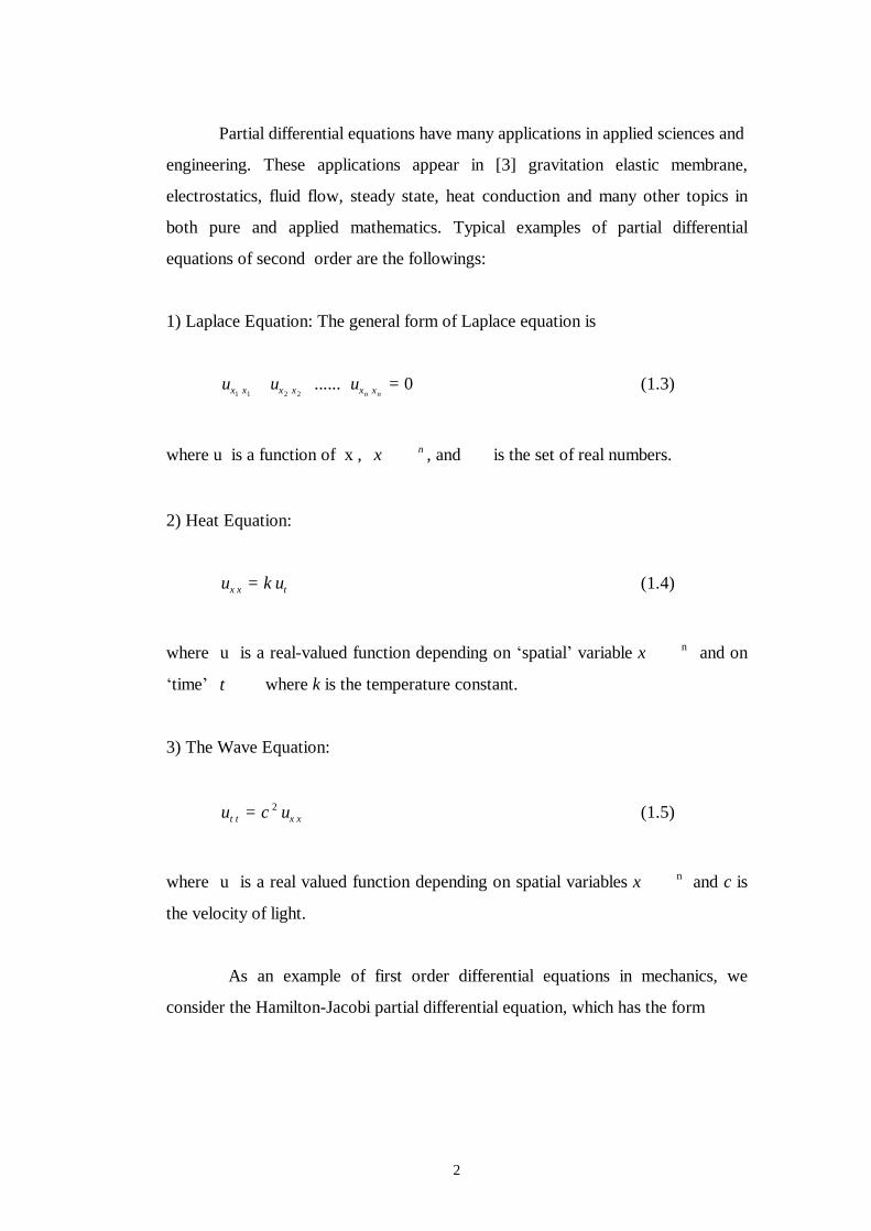
Partial differential equations have many applications in applied sciences and

engineering. These applications appear in [3] gravitation elastic membrane,

electrostatics, fluid flow, steady state, heat conduction and many other topics in

both pure and applied mathematics. Typical examples of partial differential

equations of second order are the followings:

1) Laplace Equation: The general form of Laplace equation is

u u ux x x x x xn n1 1 2 20+ + + =...... (1.3)

where u is a function of x , x n∈ℜ , and ℜ is the set of real numbers.

2) Heat Equation:

u k ux x t= (1.4)

where u is a real-valued function depending on ‘spatial’ variable x ∈ℜ n and on

‘time’ t ∈ℜ where k is the temperature constant.

3) The Wave Equation:

u c ut t x x= 2 (1.5)

where u is a real valued function depending on spatial variables x ∈ℜ n and c is

the velocity of light.

As an example of first order differential equations in mechanics, we

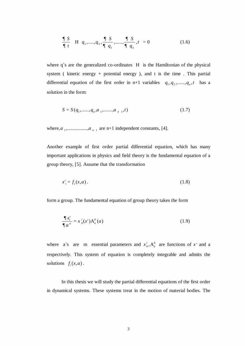
consider the Hamilton-Jacobi partial differential equation, which has the form

3

∂∂

∂∂

∂∂

St

q qSq

Sq

tnn

+

=Η 1

1

0,...., , ,....., , (1.6)

where q’s are the generalized co-ordinates H is the Hamiltonian of the physical

system ( kinetic energy + potential energy ), and t is the time . This partial

differential equation of the first order in n+1 variables q q q tn1 2, ,......, , has a

solution in the form:

S S q q tn n= +( ,......, , ,......., , )1 1 1α α (1.7)

where,α α1 1,................, n+ are n+1 independent constants, [4].

Another example of first order partial differential equation, which has many

important applications in physics and field theory is the fundamental equation of a

group theory, [5]. Assume that the transformation

x f x ai i' ( , )= . (1.8)

form a group. The fundamental equation of group theory takes the form

∂∂

ξα α

′= ′

xa

x aibi b( ) ( )Α (1.9)

where a’s are m essential parameters and ξ αbi b,Α are functions of x’ and a

respectively. This system of equation is completely integrable and admits the

solutions f x ai ( , ) .

In this thesis we will study the partial differential equations of the first order

in dynamical systems. These systems treat in the motion of material bodies. The

4

example of dynamical systems, which we will study in this thesis, are discrete and

continuous systems.

In chapter two we will investigate singular systems by a variational

principle which leads us to the canonical equations which are total differential

equations in many variables. Hence, the determination of integrability conditions of

these equations is of prime importance. In section 1 we will illustrate the relations

between the solutions of total differential equations and linear homogeneous partial

differential equations (LHPDE). Section two concerns with complete systems and

the integrability condition of the system of total differential equations. In section

three, the integration of singular system will be discussed. The equations of motion

lead us to total differential equations. Finally an example of singular system will be

studied.

In chapter three, Hamilton-Jacobi equations of the constrained dynamical

system and the integration of them will be discussed

Chapter four concerns with Hamilton-Jacobi partial differential equations of

continuous systems and the integration of them is also discussed.

5

CHAPTER II

INTEGRABILITY CONDITION OF SINGULAR SYSTEMS

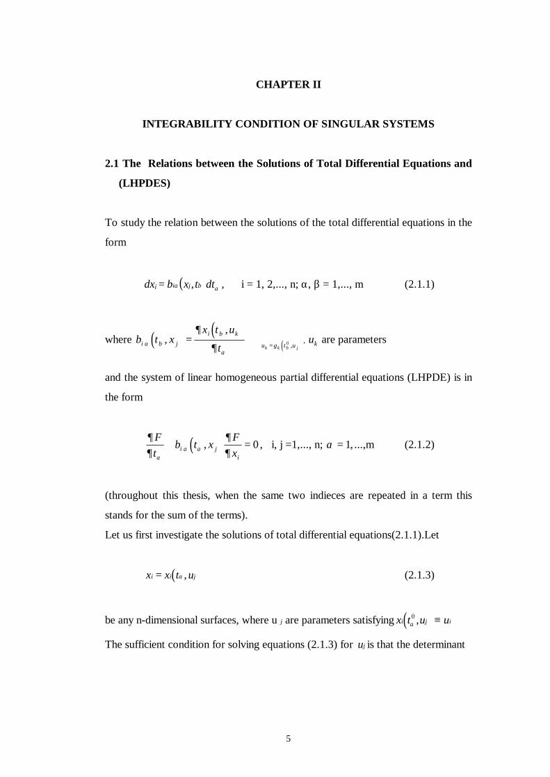
2.1 The Relations between the Solutions of Total Differential Equations and

(LHPDES)

To study the relation between the solutions of the total differential equations in the

form

dxi ( )= b x t dti jα β α, , i = 1, 2,..., n; α, β = 1,..., m (2.1.1)

where ( ) ( )b t x

x t u

ti ji k

α β

β

α

∂

∂,

,= ( )u g t uk k j= β

0 ,, uk are parameters

and the system of linear homogeneous partial differential equations (LHPDE) is in

the form

( )∂∂

∂∂α

α α

Ft

b t xFxi j

i

+ =, 0 , i, j =1,..., n; α = 1, ...,m (2.1.2)

(throughout this thesis, when the same two indieces are repeated in a term this

stands for the sum of the terms).

Let us first investigate the solutions of total differential equations(2.1.1).Let

( )x x t ui i j= α , (2.1.3)

be any n-dimensional surfaces, where u j are parameters satisfying ( )x t u ui j iα0 , ≡

The sufficient condition for solving equations (2.1.3) for uj is that the determinant

6

∂∂

xx

i

j0 0≠ , (2.1.4)

where ( )x x t u ui i j i0 0= =α , is initial point.

If condition (2.1.4) is satisfied, then one can solve (2.1.3) for u j as

( )u g t xj j i= α0 , (2.1.5)

Furthermore, the relations

( ) ( )b t x

x t u

ti ji k

α β

β

α

∂

∂,

,= ( )u g t uk k j= β

0 , (2.1.6)

hold, where biα are continuously differentiable[6]. Thus, under these conditions, we

say that ( )x x t ui i j= α , are solutions of the total differential equations (2.1.1). That

is, equation (2.1.1) are identically satisfied if we replace the xi by the expressions

(2.1.3). If m = 1, then equations (2.1.1) are ordinary differential equations. If m >1,

then biα should satisfy certain integrability conditions.

Now, we will investigate the corresponding partial differential equations of the

total differential equations (2.1.1). Differentiate equations (2.1.5) partially with

respect to tα , we have

∂

∂

∂

∂

∂

∂∂∂

∂

∂

∂

∂α α α αα

ut

gt

gx

xt

gt

gx

bj j j

i

i j j

ii= + = + (2.1.7)

Since u j is independent of tα ,

7

∂

∂

∂

∂

∂

∂∂∂

∂

∂

∂

∂α α α αα

ut

gt

gx

xt

gt

gx

bj j j

i

i j j

ii= + = + = 0 (2.1.8)

which is the same form of equations (2.1.2). Now, we want to determine the

necessary and sufficient condition for the system of total differential equations

(2.1.1) to be completely integrable [6]. To do this, let us consider the following

theorem:

Theorem 2.1.1

The necessary and sufficient condition for the system of total differential equations

(2.1.1) to be completely integrable is that

∂

∂

∂

∂

∂

∂

∂

∂α

β

β

α

αβ

βα

bt

bt

bx

bbx

bi i i

jj

i

jj− + − = 0 (2.1.9)

Proof

Let us consider a point in (n+m) dimensional space formed by ( , )t xiα , and set

t t sα α αλ= +0 (2.1.10)

where s is an arbitrary variable, and λ α ’s are parameters. Thus we can express

the total differential equation (2.1.1) as a set of ordinary differential equations with

m parameters λ α as follows:

The system of total differential equations (2.1.1) becomes

( ) ( ) ( )dx b t s x d t s b t s x dsi i j i j= + + = +α β β α α α β β αλ λ λ λ0 0 0, , (2.1.11)

8

hence

( )dxds

b t s xii j= +λ λα α β β

0 , (2.1.12)

These are ordinary differential equations and their solutions are functions of s ,

arbitrary parameters λ α , and the initial values u j , i.e

( )x s ui i j= ϕ λ α, , (2.1.13)

Hence ,

( )u uj j i≡ ϕ λ α0, , (2.1.14)

or

( )u s uj j i≡ ϕ , ,0 (2.1.15)

Thus , by using equations (2.1.10), the equations (2.1.13) take the form:

( )x t u st t

sui j i jα

α αϕ, , ,=−

0

(2.1.16)

Since the left hand side of equations (2.1.16) is independent of s , the right hand

side also should be independent of s. Under the assumption that s ≠0, the above

requirement means

d xd s s s u

us

i i i i

j

j= + + =∂ϕ∂

∂ϕ∂ λ

∂ λ∂

∂ϕ∂

∂

∂α

α 0 (2.1.17)

9

Since ∂

∂

us

j = 0 , and by using (2.1.10), we have

∂ϕ∂

∂ϕ∂ λ

α α

α

i i

st t

s−

−=

0

2 0 (2.1.18)

or

ss

i i∂ϕ∂

λ∂ϕ∂λα

α

− = 0 (2.1.19)

Now, let us differentiate the equation (2.1.16) partially with respect to tα ,

we will obtain,

∂∂

∂ϕ∂

∂∂

∂ϕ∂ λ

∂ λ

∂∂ϕ∂

∂

∂α α β

β

α α

xt s

st t u

ut

i i i i

j

j= + + (2.1.20)

with

∂ λ

∂δ

∂∂

∂

∂β

αα β

α αt sst

andut

j= = =1

0 0, , , equation (2.1.20) becomes

∂∂

∂ϕ∂ λα α

xt s

si i= ≠1 0, (2.1.21)

Using equations (2.1.6), we shall get

∂ϕ∂λ

λ ϕα

α β βi

i jsb t s= +( , )0 (2.1.22)

10

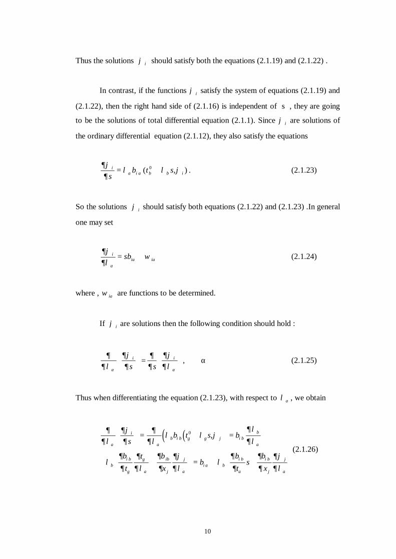
Thus the solutions ϕ i should satisfy both the equations (2.1.19) and (2.1.22) .

In contrast, if the functions ϕ i satisfy the system of equations (2.1.19) and

(2.1.22), then the right hand side of (2.1.16) is independent of s , they are going

to be the solutions of total differential equation (2.1.1). Since ϕ i are solutions of

the ordinary differential equation (2.1.12), they also satisfy the equations

∂ϕ∂

λ λ ϕα α β βi

i isb t s= +( , )0 . (2.1.23)

So the solutions ϕ i should satisfy both equations (2.1.22) and (2.1.23) .In general

one may set

∂ϕ∂λ

ωα

α αi

i isb= + (2.1.24)

where , ω αi are functions to be determined.

If ϕ i are solutions then the following condition should hold :

∂∂ λ

∂ϕ∂

∂∂

∂ϕ∂ λα α

i i

s s

=

, ∀α (2.1.25)

Thus when differentiating the equation (2.1.23), with respect to λ α , we obtain

( )( )∂

∂ λ∂ϕ∂

∂∂λ

λ λ ϕ∂ λ

∂ λ

λ∂

∂

∂

∂ λ

∂

∂

∂ϕ

∂ λλ

∂

∂

∂

∂

∂ϕ

∂ λ

α αβ β γ γ β

β

α

ββ

γ

γ

α

β

αα β

β

α

β

α

ii j i

i i

j

ji

i i

j

j

sb t s b

bt

t bx

bbt

sbx

= + =

+ +

= + +

0 ,

(2.1.26)

11

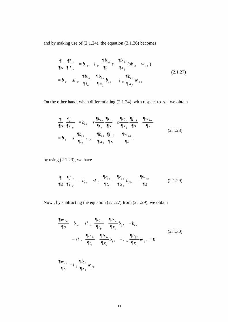
and by making use of (2.1.24), the equation (2.1.26) becomes

∂∂

∂ϕ∂ λ

λ∂

∂

∂

∂ω

λ∂

∂

∂

∂λ

∂

∂ω

αα β

β

α

βα α

α ββ

α

βα β

βα

sb

bt

sbx

sb

b sbt

bx

bbx

ii

i i

jj j

ii i

jj

i

jj

= + + +

= + +

+

( )

(2.1.27)

On the other hand, when differentiating (2.1.24), with respect to s , we obtain

∂∂

∂ϕ∂ λ

∂

∂

∂

∂

∂

∂

∂ϕ

∂

∂ω

∂

∂

∂λ

∂

∂

∂ϕ

∂

∂ω

∂

αα

α

β

β α α

αα

ββ

α α

sb s

bt

ts

sbx s s

b sbt

bx s s

ii

i i

j

j i

ii i

j

j i

= + + +

= + +

+ .

(2.1.28)

by using (2.1.23), we have

∂∂

∂ϕ∂ λ

λ∂

∂

∂

∂

∂ω

∂αα β

α

β

αβ

α

sb s

bt

bx

bs

ii

i i

jj

i

= + +

+ (2.1.29)

Now , by subtracting the equation (2.1.27) from (2.1.29), we obtain

∂ω

∂λ

∂

∂

∂

∂

λ∂

∂

∂

∂λ

∂

∂ω

αα β

α

β

αβ α

ββ

α

βα β

βα

ii

i i

jj i

i i

jj

j

jj

sb s

bt

bx

b b

sbt

bx

bbx

+ + +

−

− +

− = 0

(2.1.30)

∂ω

∂λ

∂

∂ωα

ββ

αi i

jjs

bx

−

12

= sbt

bt

bx

bbx

b si i i

jj

i

jj iλ

∂

∂

∂

∂

∂

∂

∂

∂λβ

β

α

α

β

βα

αβ β β α− + −

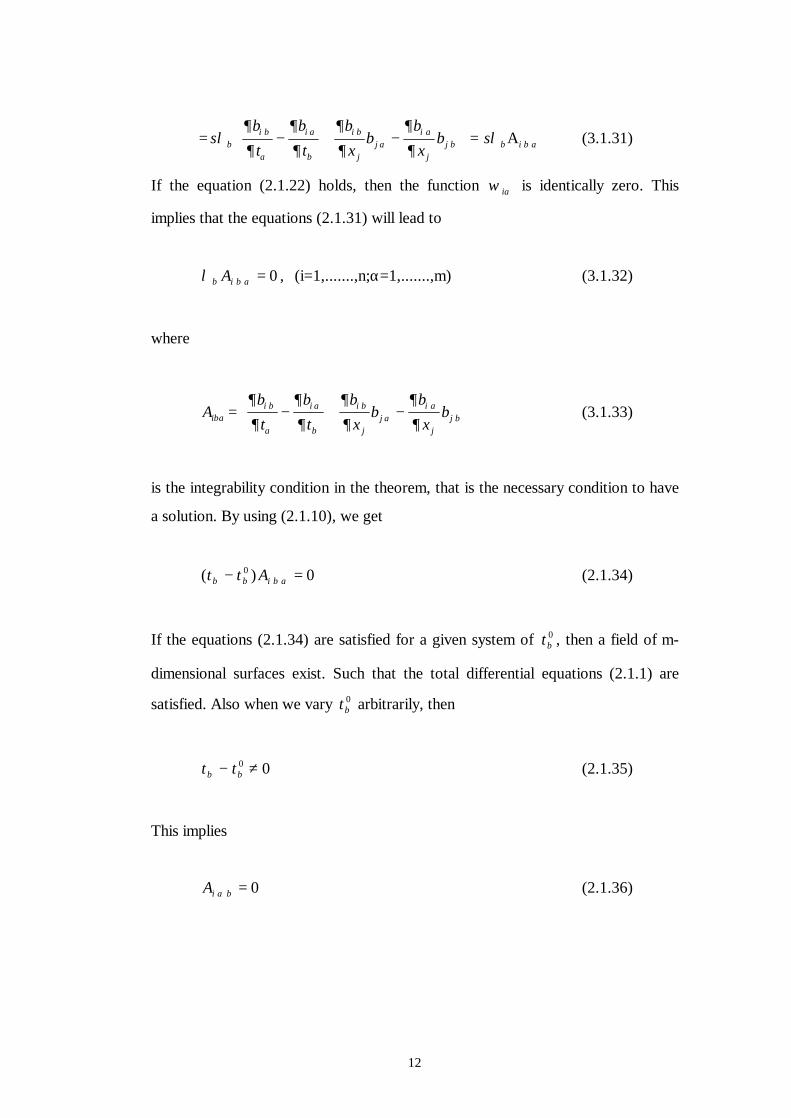
= Α (3.1.31)

If the equation (2.1.22) holds, then the function ω αi is identically zero. This

implies that the equations (2.1.31) will lead to

λ β β αAi = 0 , (i=1,.......,n;α=1,.......,m) (3.1.32)

where

Aiβα =∂

∂

∂

∂

∂

∂

∂

∂β

α

α

β

βα

αβ

bt

bt

bx

bbx

bi i i

jj

i

jj− + −

(3.1.33)

is the integrability condition in the theorem, that is the necessary condition to have

a solution. By using (2.1.10), we get

( )t t Aiβ β β α− =0 0 (2.1.34)

If the equations (2.1.34) are satisfied for a given system of tβ0 , then a field of m-

dimensional surfaces exist. Such that the total differential equations (2.1.1) are

satisfied. Also when we vary tβ0 arbitrarily, then

t tβ β− ≠0 0 (2.1.35)

This implies

Ai α β = 0 (2.1.36)

13

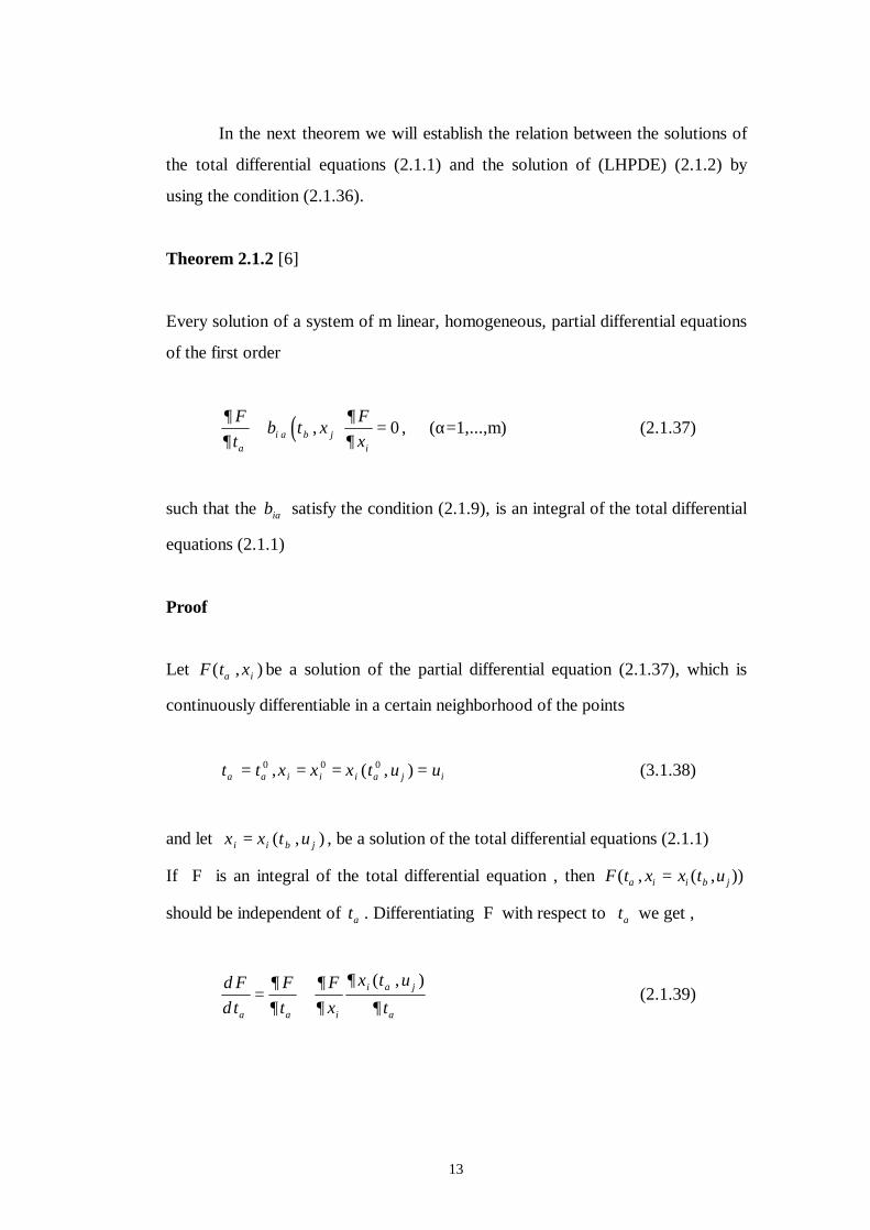
In the next theorem we will establish the relation between the solutions of

the total differential equations (2.1.1) and the solution of (LHPDE) (2.1.2) by

using the condition (2.1.36).

Theorem 2.1.2 [6]

Every solution of a system of m linear, homogeneous, partial differential equations

of the first order

( )∂∂

∂∂α

α β

Ft

b t xFxi j

i

+ =, 0 , (α=1,...,m) (2.1.37)

such that the biα satisfy the condition (2.1.9), is an integral of the total differential

equations (2.1.1)

Proof

Let F t xi( , )α be a solution of the partial differential equation (2.1.37), which is

continuously differentiable in a certain neighborhood of the points

t t x x x t u ui i i j iα α α= = = =0 0 0, ( , ) (3.1.38)

and let x x t ui i j= ( , )β , be a solution of the total differential equations (2.1.1)

If F is an integral of the total differential equation , then F t x x t ui i j( , ( , ))α β=

should be independent of tα . Differentiating F with respect to tα we get ,

d Fd t

Ft

Fx

x t uti

i j

α α

α

α

∂∂

∂∂

∂

∂= +

( , ) (2.1.39)

14

Since x x t ui i j= ( , )α is a solution, it satisfies

∂

∂α

α

x t ut

i j( , ) u gj j= = bi α (2.1.40)

Then

d Fd t

Ft

bFxi

iα αα

∂∂

∂∂

= + = 0 , ∀α (2.1.41)

Hence , F is independent of tα .According to (2.1.5) , we write

F t x t u u g t xi j j j i( , ( , )) ( ) ( ( , )α β αϕ ϕ= = (2.1.42)

Conversely, for any function ϕ( )g ýj , we have

dd t g

gt g

gx

x t ut g

gt

gx

xtj

j

j

j

i

i j

j

j j

i

iϕ ∂ϕ∂

∂

∂∂ϕ∂

∂

∂

∂

∂∂ϕ∂

∂

∂

∂

∂∂∂α α

β

α α α

= + = +

( , )(2.1.43)

By using (2.1.40) , we obtain

ddt

ϕ

α

= 0 (2.1.44)

This means that every function ϕ ( )g j is a solution of (2.1.37) .

Hence we conclude that , a complete manifold of solutions of LHPDE with

more than one independent variable can be obtained by the functionally

15

independent integrals of corresponding total differential equation in analogy with

the case of one independent variables .

2.2 Complete System of LHPDES of the First Order

In this section we would like to define a complete system of partial differential

equations and its solution . Consider the system of linear partial differential

equation.

a xfx

m i j ni ji

α

∂∂

α( ) , ( ,..... , ; , ,...... , )= = =0 1 1 (2.2.1)

where m are linearly independent equations. Here, linear independence means that

the rank of the determinant a iα is m.

To find the solutions, let us define the linear operators Χα , as [6]

Χα α

∂∂

f a xfxi j

i

= =( ) 0 (2.2.2)

These linear operators Χα f satisfy the following relations :

Χ

Χ Χ

α α

α α α α

∂∂

∂∂

∂∂

( ) ( ) ( )

( ) ( )

f g a x f gx

a xfx

a xgx

f g

i ji

i ji

i ji

+ =+

= + = + (2.2.3)

Also

Χ Χ Χα α α α α α

∂∂

∂∂

∂∂

fg a fgx

gafx

fa gx

g f f gii

ii

ii

= = + = +( ) (2.2.4)

16

Now we want to define the bracket of two operators Χ Χα βand .Let us

evaluate

( )

Χ Χ Χ Χ Χ

Χ

β α β α β α α β

β α α β

∂∂

∂∂

∂∂

∂∂

∂∂ ∂

f afx

afx

afx

afx

a a fx x

ii

ii

ii

ii

i ji j

= = +

= +

( ) ( )

2 (2.2.5)

and

( )Χ Χ Χα β α β β α

∂∂

∂∂ ∂

f a fx

a a fx xi

ii j

j i

= +2

(2.2.6)

Now, the symmetry between α and β implies that

a a fx x

a a fx xi j

i ji j

j iα β β α

∂∂ ∂

∂∂ ∂

2 2

= (2.2.7)

Setting the bracket

( ) ( )

( )Χ Χ Χ Χ Χ Χ

Χ Χ Χ Χ Χ Χ

α β α β β α

α β β α α β β α

∂∂

, f f

f f a a fxi i

i

= −

= − = − (2.2.8)

One should notice that

( )Χ Χα β, f = 0 (2.2.9)

represents a set of LHPDE in the form (2.2.1) .

17

Definition 2.2.1

A system of partial differential equations

Χα α

∂∂

f b fxi

i

= (2.2.10)

is called complete if the following relations hold,

( )Χ Χ Χα β αβγ, f fcc= , (α, β, c = 1,.........., m) (2.2.11)

when γ αβc ’s are functions of x j ’s [5], [6].

In other words if the system is complete, the bracket of any two operators can be

written as a linear combination of the operators .So every twice differential

solutions of the equations (2.2.2) should satisfy m(m-1)/2 relations (2.2.9) .The

conclusion is that a complete system , and the linear system (2.2.10) have the same

solutions .Also from the bracket relations (2.2.11), we can obtain the maximum

number of linearly independent equations .

Since the rank of the matrix is m, there are m linearly independent

equations, which satisfy the relation (2.2.9).

If m = n the only solution of equation (2.2.10) is f = constant. .If m < n

there is a possibility of solutions other than the trivial one. Now , if the equations

(2.2.11) hold , then we adjoin this type of relations with relation (2.2.10) and we

have

s ≥ m linearly independent equations . If s >m, we repeat this process and obtain

a system of s` ≥ s linearly independent equations . If s` > s , we continue

18

this process. Finally we have either n independent equations , and the only

solution in this case is f = constant, or we get a number u less than n for which

α,β,c in (2.2.11) take the values 1,.......,u .

In the first case , we say that the system (2.2.10) is complete of order n and in the

other case of order u .

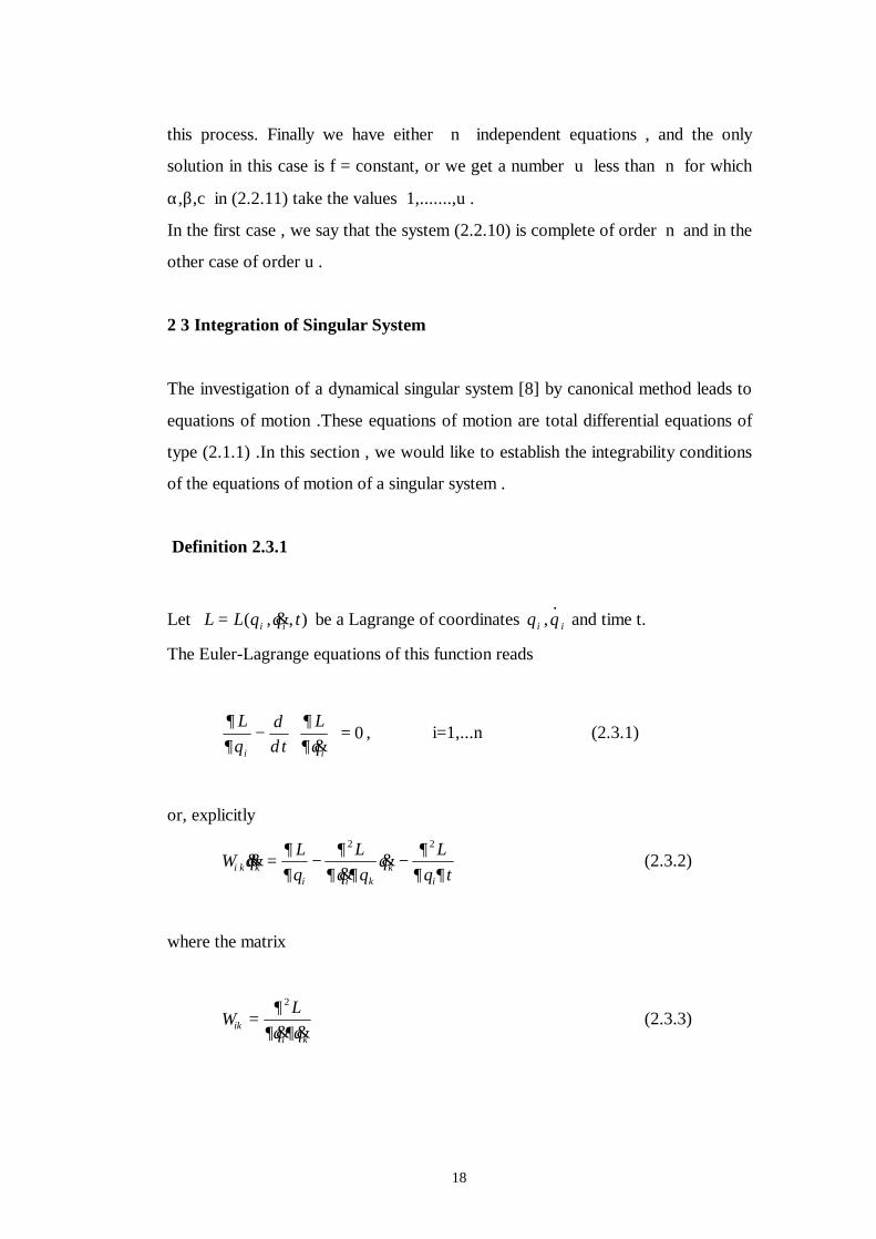
2 3 Integration of Singular System

The investigation of a dynamical singular system [8] by canonical method leads to

equations of motion .These equations of motion are total differential equations of

type (2.1.1) .In this section , we would like to establish the integrability conditions

of the equations of motion of a singular system .

Definition 2.3.1

Let L L q q ti i= ( , & , ) be a Lagrange of coordinates q qi i,.

and time t.

The Euler-Lagrange equations of this function reads

∂∂

∂∂

Lq

dd t

Lqi i

−

=

&0 , i=1,...n (2.3.1)

or, explicitly

W qLq

Lq q

qL

q ti k ki i k

ki

&&&

&= − −∂∂

∂∂ ∂

∂∂ ∂

2 2

(2.3.2)

where the matrix

WL

q qiki k

=∂

∂ ∂

2

& & (2.3.3)

19

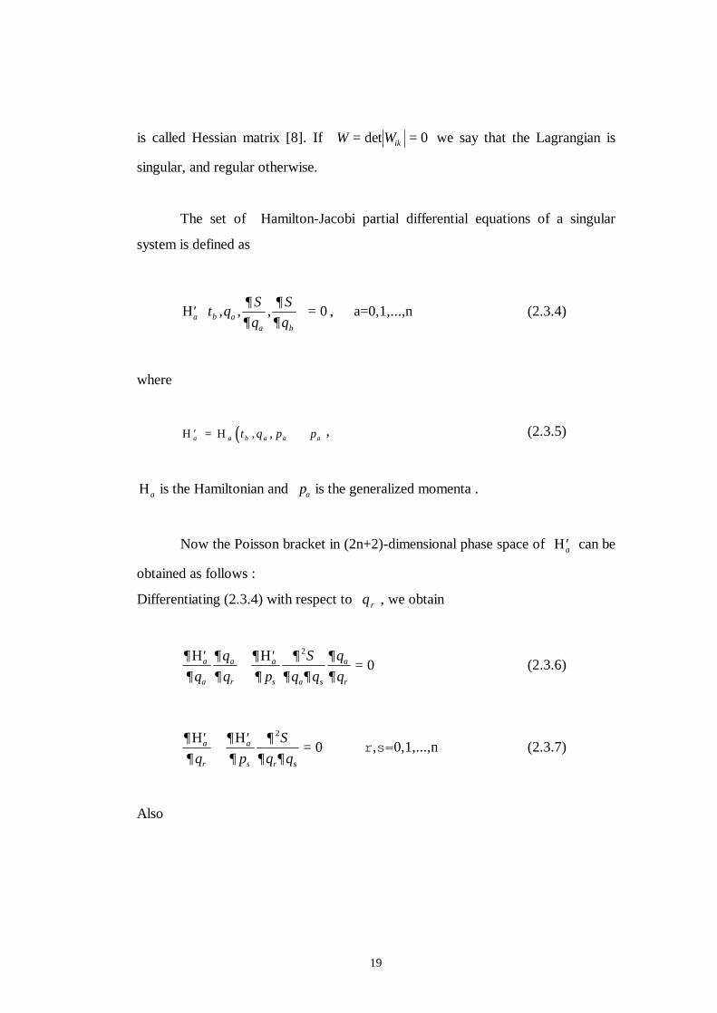
is called Hessian matrix [8]. If W Wik= =det 0 we say that the Lagrangian is

singular, and regular otherwise.

The set of Hamilton-Jacobi partial differential equations of a singular

system is defined as

′

=Ηα β

β

∂∂

∂∂

t q Sq

Sqa

a

, , , 0 , a=0,1,...,n (2.3.4)

where

( )′ = +Η Ηα α β α αt q p pa, , , (2.3.5)

Ηα is the Hamiltonian and pα is the generalized momenta .

Now the Poisson bracket in (2n+2)-dimensional phase space of ′Ηα can be

obtained as follows :

Differentiating (2.3.4) with respect to q r , we obtain

∂∂

∂∂

∂∂

∂∂ ∂

∂∂

α α′+

′=

Η Ηq

qq p

Sq q

qqa

a

r s a s

a

r

2

0 (2.3.6)

∂∂

∂∂

∂∂ ∂

α α′+

′=

Η Ηq p

Sq qr s r s

2

0 ∀r,s=0,1,...,n (2.3.7)

Also

20

∂

∂

∂

∂∂

∂ ∂β β′

+′

=Η Η

q pS

q qr s r s

2

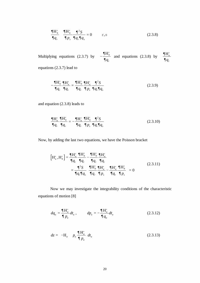
0 ∀r,s (2.3.8)

Multiplying equations (2.3.7) by −′∂

∂βΗ

qr

and equations (2.3.8) by ∂∂

α′Ηqr

equations (2.3.7) lead to

−′ ′

=′ ′∂

∂∂∂

∂

∂∂∂

∂∂ ∂

β α β αΗ Η Η Ηq q q p

Sq qr r r s r s

2

(2.3.9)

and equation (2.3.8) leads to

∂∂

∂

∂∂∂

∂

∂∂

∂ ∂α β α β′ ′

= −′ ′Η Η Η Η

q q q pS

q qr r r s r s

2

(2.3.10)

Now, by adding the last two equations, we have the Poisson bracket

[ ]′ ′ =

′ ′−

′ ′

=′ ′

−′ ′

=

Η ΗΗ Η Η Η

Η Η Η Η

α βα β β α

β α α β

∂∂

∂

∂

∂

∂∂∂

∂∂ ∂

∂

∂∂∂

∂∂

∂

∂

,q q q q

Sq q q p q p

r r r r

r s r s r s

2

0 (2.3.11)

Now we may investigate the integrability conditions of the characteristic

equations of motion [8]

dqp

dtaa

=′∂

∂α

α

Η , dpq

dtaa

= −′∂

∂α

α

Η (2.3.12)

dz pp

dta

= − +′

Η

Ηα α

αα

∂∂

(2.3.13)

21

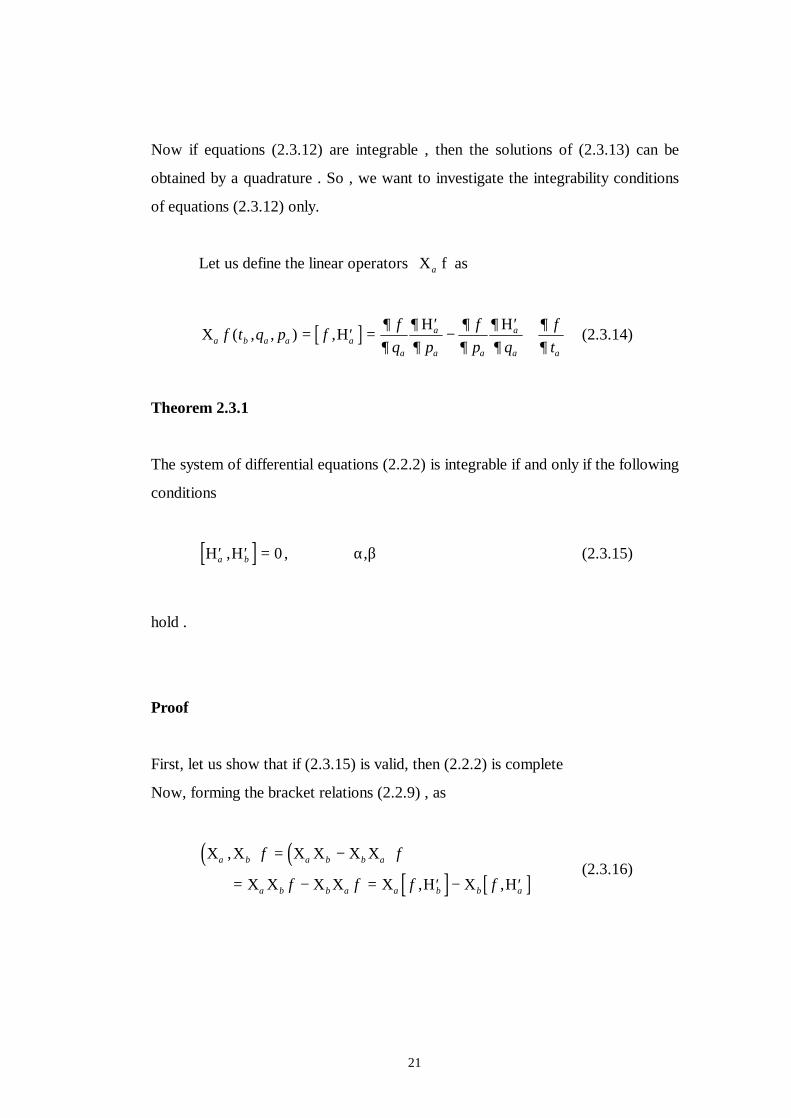
Now if equations (2.3.12) are integrable , then the solutions of (2.3.13) can be

obtained by a quadrature . So , we want to investigate the integrability conditions

of equations (2.3.12) only.

Let us define the linear operators Χα f as

[ ]Χ ΗΗ Η

α β αα α

α

∂∂

∂∂

∂∂

∂∂

∂∂

f t q p f fq p

fp q

fta a

a a a a

( , , ) ,= ′ =′

−′

+ (2.3.14)

Theorem 2.3.1

The system of differential equations (2.2.2) is integrable if and only if the following

conditions

[ ]′ ′ =Η Ηα β, 0 , ∀α,β (2.3.15)

hold .

Proof

First, let us show that if (2.3.15) is valid, then (2.2.2) is complete

Now, forming the bracket relations (2.2.9) , as

( ) ( )

[ ] [ ]Χ Χ Χ Χ Χ Χ

Χ Χ Χ Χ Χ Η Χ Η

α β α β β α

α β β α α β β α

,

, ,

f f

f f f f

= −

= − = ′ − ′ (2.3.16)

22

( ) [ ][ ] [ ][ ]Χ Χ Η Η Η Ηα β β α α β, , , , ,f f f= ′ ′ − ′ ′ (2.3.17)

Making use of the Jacobi relations

[ ][ ] [ ][ ] [ ][ ]f f f, , , , , ,′ ′ + ′ ′ + ′ ′Η Η Η Η Η Ηβ α α β β α =0 (2.3.18)

we have

[ ][ ] [ ][ ]f f, , , ,′ ′ = − ′ ′Η Η Η Ηα β α β (2.3.19)

and relation (2.3.17) becomes

( ) [ ][ ]Χ Χ Η Ηα β β α, , ,f f+ ′ ′

= [ ][ ] [ ][ ] [ ][ ]f f f, , , , , ,′ ′ + ′ ′ + ′ ′Η Η Η Η Η Ηβ α α β β α =0 (2.3.20)

This implies

( ) [ ][ ] [ ][ ]Χ Χ Η Η Η Ηα β β α β α, , , , ,f f f= − ′ ′ = ′ ′ (2.3.21)

Identifying

[ ] ( )′ ′ = =Η Η Αβ α βα, , ,t q pj a a 0 , (2.3.22)

then

( ) [ ]Χ Χ ΑΑ Α

α β β αβ α β α∂

∂

∂

∂

∂

∂∂∂

, ,f ff

q p qf

pa a a a

= = − = 0 (2.3.23)

23

and the system is complete .

conversely, if the system (2.2.2) is integrable, then it completes[5],[6] , this

implies, due to the equation (2.3.23) , that

( ) [ ]Χ Χ ΑΑ Α

α β αβαβ αβ∂

∂

∂

∂

∂

∂∂∂

, ,f f fq p q

fpa a a a

= = − = 0 (2.3.24)

Then

∂

∂

∂

∂αβ αβΑ Α

p qa a

= = 0 (2.3.25)

Thus (2.3.15) is hold, and this is the end of the proof of this theorem.

.

Now , if the integrability conditions are satisfied , then the solutions of the

total differential equations (2.3.12) and (2.3.13) are obtained as

( )q t ua a b= ξ α , , ( )p t ua a b= η α , , ( )z t ub= σ α , (2.3.26)

where ua are arbitrary parameters .

The function

( )z S t q a= α , (2.3.27)

is obtained by solving (2.3.13)

Now, if

24

( ) ( )Λ Ηα β α βα

ξ η η∂ξ∂

t u tta a a a

a, , ,= − + (2.3.28)

then the equation (2.3.13) leads to

dz dt= Λα α (2.3.29)

and this equation is a total differential equation and its solution is

( )σ α α α αt u s u dta, ( )= + ∫ Λ (2.3.30)

Example 2.3.1

Consider a dynamical system of Hamiltonians defined as [6], [8],

Η 012

1

32

2

1 2= −

+/

pa

pa

c (2.3.31)

Η 2 3= −p b (2.3.32)

when a a b1 2, , are constants , and c q( )1 is a function of q1 .

The set of HJPDE (2.3.4) is

∂∂τ

τ∂∂

∂∂

Sq p

Sq

pSqi+ = =

=Η0 1

13

3

0, , , (2.3.33)

∂∂

τ∂∂

∂∂

Sq

q pSq

pSqi

22 1

13

3

0+ = =

=Η , , , (2.3.34)

According to the last theorem, the system is integrable if and only if

25

[ ]′ ′ =Η Η0 2 0, , (2.3.35)

that is

[ ] [ ]′ ′ = + +Η Η Η Η0 2 0 0 2 2, ,p p = − +∂∂τ

∂∂

∂∂

∂∂

Η Η Η Η2 0

2

0

1

2

1q q p

+ − − =∂∂

∂∂

∂∂

∂∂

∂∂

∂∂

Η Η Η Η Η Η0

3

2

3

0

1

2

1

0

3

2

3

0q p p q p q

(2.3.36)

Now, we going to show that

( )Χ Χ0 2 0, f = (2.3.37)

By using definition (2.3.14), we have

( ) [ ] [ ]

[ ][ ] [ ][ ]Χ Χ Χ Χ Χ Χ Χ Η Χ Η

Η Η Η Η0 2 0 2 2 0 0 2 2 0

2 0 0 2

, , ,

, , , ,

f f f f f

f f

= − = ′ − ′

= ′ ′ − ′ ′ (2.3.38)

Making use of Jacobi relation

[ ][ ] [ ][ ] [ ][ ]f f f, , , , , ,′ ′ + ′ ′ + ′ ′Η Η Η Η Η Η2 0 0 2 0 =0 (2.3.39)

the bracket (2.3.38)becomes

( ) [ ][ ] [ ][ ] [ ][ ]

[ ][ ] [ ][ ] [ ][ ] [ ][ ]Χ Χ Η Η Η Η Η Η

Η Η Η Η Η Η Η Η

0 2 2 0 2 0 0 2

2 0 2 0 0 2 2 0 0

, , , , , , ,

, , , , , , , ,

f f f f

f f f f

+ ′ ′ = ′ ′ − ′ ′

+ ′ ′ = ′ ′ + ′ ′ + ′ ′ = (2.3.40)

Then

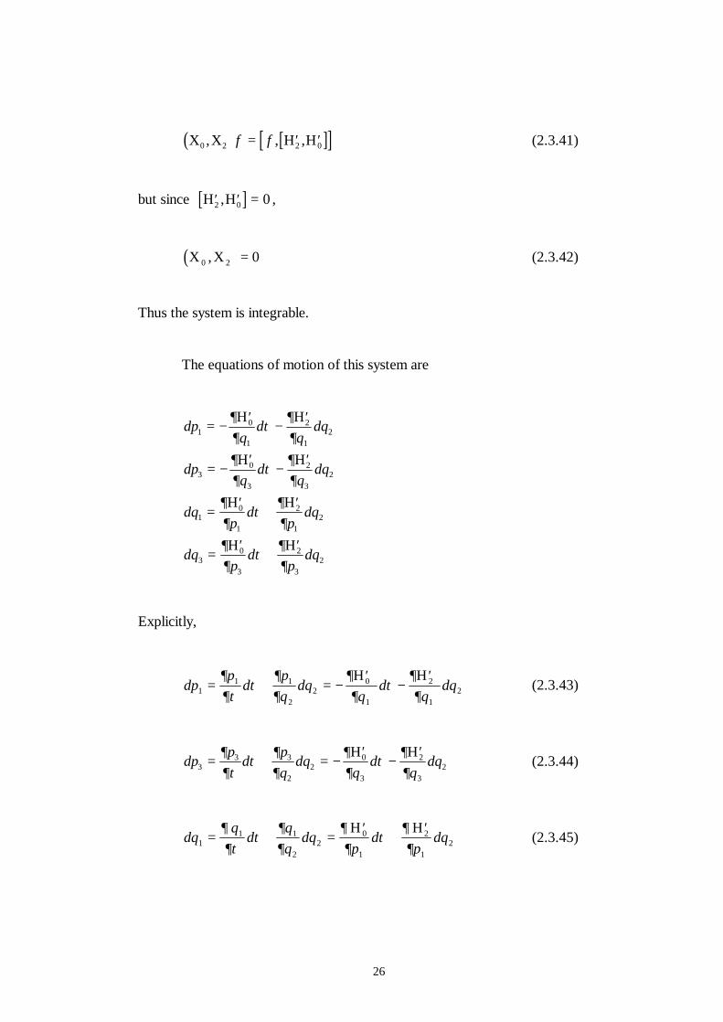
26

( ) [ ][ ]Χ Χ Η Η0 2 2 0, , ,f f= ′ ′ (2.3.41)

but since [ ]′ ′ =Η Η2 0 0, ,

( )Χ Χ0 2 0, = (2.3.42)

Thus the system is integrable.

The equations of motion of this system are

dpq

dq

dq

dpq

dq

dq

dqp

dp

dq

dqp

dp

dq

10

1

2

12

30

3

2

32

10

1

2

12

30

3

2

32

= −′

−′

= −′

−′

=′

+′

=′

+′

∂∂

τ∂∂

∂∂

τ∂∂

∂∂

τ∂∂

∂∂

τ∂∂

Η Η

Η Η

Η Η

Η Η

Explicitly,

dpp

dpq

dqq

dq

dq11 1

22

0

1

2

12= + = −

′−

′∂∂τ

τ∂∂

∂∂

τ∂∂

Η Η (2.3.43)

dp p d pq

dqq

dq

dq33 3

22

0

3

2

32= + = −

′−

′∂∂τ

τ∂∂

∂∂

τ∂∂

Η Η (2.3.44)

dqq

dqq

dqp

dp

dq11 1

22

0

1

2

12= + =

′+

′∂∂τ

τ∂∂

∂∂

τ∂∂

Η Η (2.3.45)

27

dq q d qq

dqp

dp

dq33 3

22

0

3

2

32= + =

′+

′∂∂ τ

τ∂∂

∂∂

τ∂∂

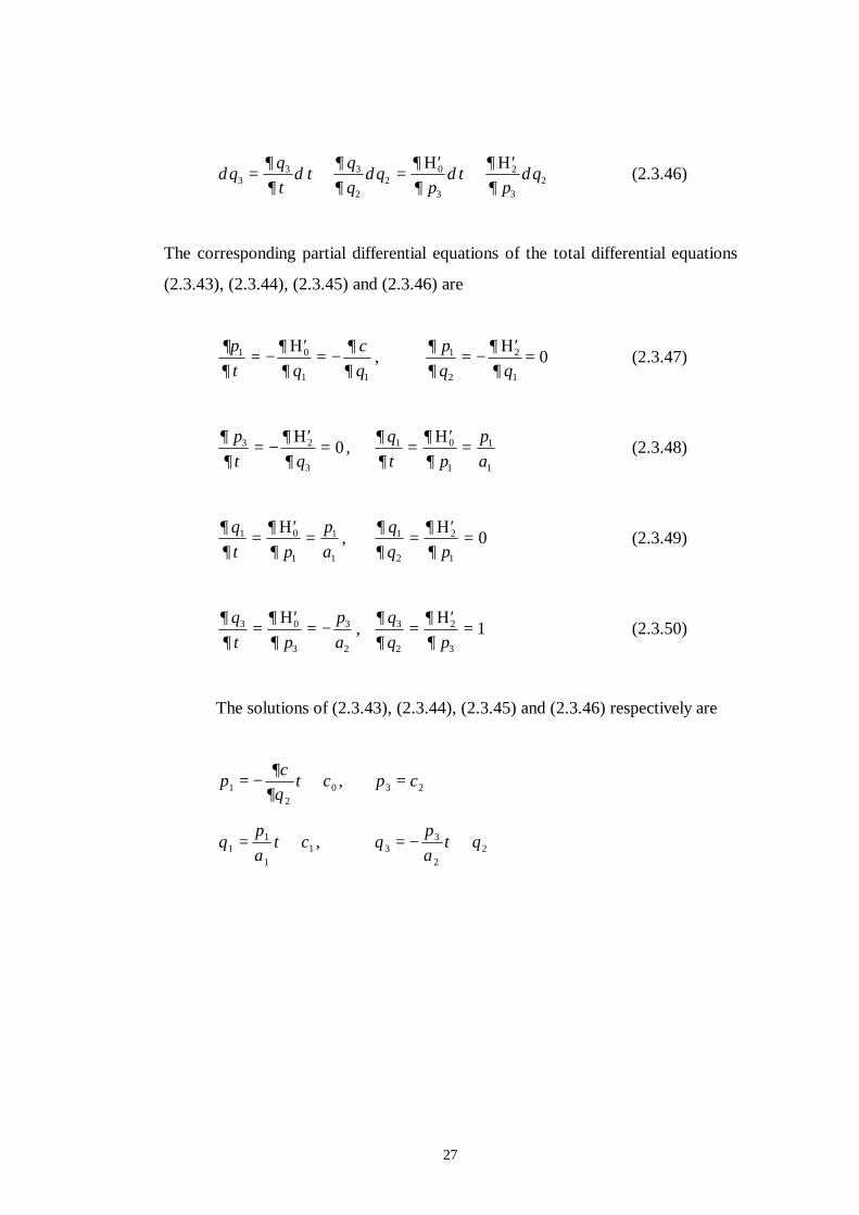
Η Η (2.3.46)

The corresponding partial differential equations of the total differential equations

(2.3.43), (2.3.44), (2.3.45) and (2.3.46) are

∂∂ τ

∂∂

∂∂

pq

cq

1 0

1 1

= −′

= −Η , ∂

∂∂∂

pq q

1

2

2

1

= −′Η = 0 (2.3.47)

∂∂ τ

∂∂

pq

3 2

3

0= −′

=Η , ∂

∂ τ∂∂

qp

pa

1 0

1

1

1

=′

=Η (2.3.48)

∂∂ τ

∂∂

qp

pa

1 0

1

1

1

=′

=Η , ∂

∂∂∂

qq p

1

2

2

1

0=′

=Η (2.3.49)

∂∂ τ

∂∂

qp

pa

3 0

3

3

2

=′

= −Η , ∂

∂∂∂

qq p

3

2

2

3

1=′

=Η (2.3.50)

The solutions of (2.3.43), (2.3.44), (2.3.45) and (2.3.46) respectively are

p cq

c12

0= − +∂

∂τ , p c3 2=

qpa

c11

11= +τ , q

pa

q33

22= − +τ

29

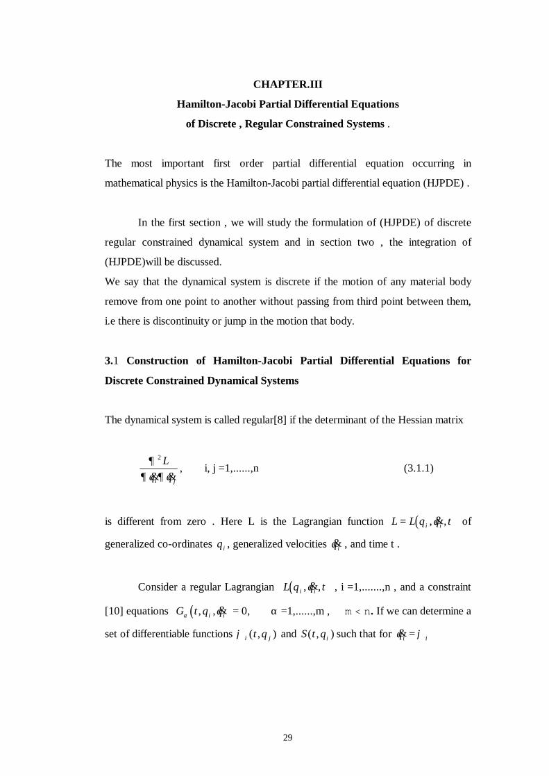
CHAPTER.III

Hamilton-Jacobi Partial Differential Equations

of Discrete , Regular Constrained Systems .

The most important first order partial differential equation occurring in

mathematical physics is the Hamilton-Jacobi partial differential equation (HJPDE) .

In the first section , we will study the formulation of (HJPDE) of discrete

regular constrained dynamical system and in section two , the integration of

(HJPDE)will be discussed.

We say that the dynamical system is discrete if the motion of any material body

remove from one point to another without passing from third point between them,

i.e there is discontinuity or jump in the motion that body.

3.1 Construction of Hamilton-Jacobi Partial Differential Equations for

Discrete Constrained Dynamical Systems

The dynamical system is called regular[8] if the determinant of the Hessian matrix

∂

∂ ∂

2 Lq qi j& &

, i, j =1,......,n (3.1.1)

is different from zero . Here L is the Lagrangian function ( )L L q q ti i= , & , of

generalized co-ordinates q i , generalized velocities &q i , and time t .

Consider a regular Lagrangian ( )L q q ti i, & , , i =1,.......,n , and a constraint

[10] equations ( )G t q qi iα , , & ,= 0 α =1,......,m , m < n. If we can determine a

set of differentiable functions ϕ i jt q( , ) and S t qi( , ) such that for &q i i= ϕ

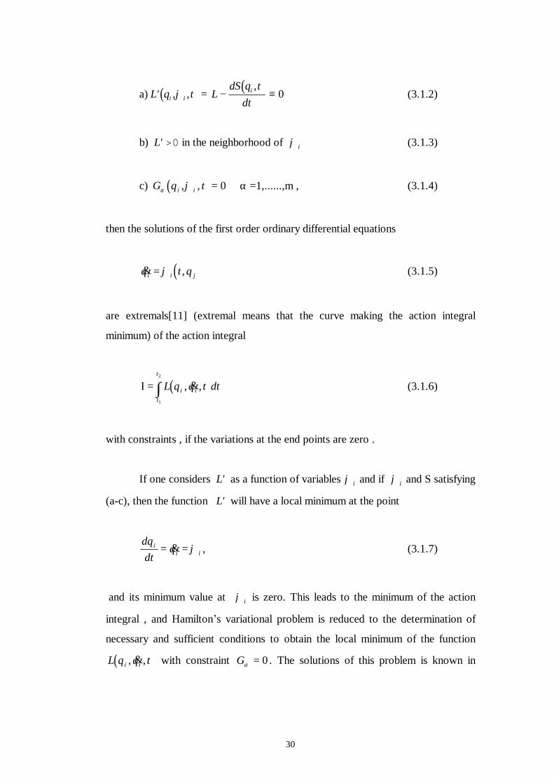
30

a) ( ) ( )′ = − ≡L q t L

dS q tdti i

i, ,,

ϕ 0 (3.1.2)

b) ′L >0 in the neighborhood of ϕ i (3.1.3)

c) ( )G q ti iα ϕ, , = 0 α =1,......,m , (3.1.4)

then the solutions of the first order ordinary differential equations

( )& ,q t qi i j= ϕ (3.1.5)

are extremals[11] (extremal means that the curve making the action integral

minimum) of the action integral

( )Ι = ∫ L q q t dti it

t

, & ,1

2

(3.1.6)

with constraints , if the variations at the end points are zero .

If one considers ′L as a function of variables ϕ i and if ϕ i and S satisfying

(a-c), then the function ′L will have a local minimum at the point

dqdt

qii i= =& ,ϕ (3.1.7)

and its minimum value at ϕ i is zero. This leads to the minimum of the action

integral , and Hamilton’s variational problem is reduced to the determination of

necessary and sufficient conditions to obtain the local minimum of the function

( )L q q ti i, & , with constraint Gα = 0 . The solutions of this problem is known in

31

terms of Lagrange multipliers. If instead of the Lagrangian L, one starts with a

function

( ) ( ) ( )Μ t q q L t q q t G t q qi i i i i i, , & , & , , & & ( ) , , &λ λα α α= + (3.1.8)

then the extremum problem with constraint is reduced to the ordinary extremum

problem. Here &λ α are the Lagrange multipliers [12] to be determined .In this new

formulation the previous Caratheodory’s equivalent Lagrangian [10] method can

be rewritten as follows:

Consider a function ( )Μ t q qi i, , & , &λ α . If it is possible to determine n+p ,

differentiable function ( )η ρ σt q, , ρ,σ =1,......n+p, and function ( )S q tρ ,

such that

a) ( ) ( )′ = − − ≡Μ Μt q t q Sq

Sti i, , , ,η η

∂∂

η∂∂ρ ρ

ρρ 0 (3.1.9)

b) ′Μ >0 in the neighbourhood , (3.1.10)

then the solutions of the system of first order ordinary differential equations

( )dqdt

t qρρ ρη= , (3.1.11)

are the extremals of the action integral (3.1.6), with constraint equations

( )G t q qi iα , , & = 0 (3.1.12)

32

Proposition 3.1.1 [10]

The necessary condition for the function ′Μ to have a local minimum value zero

at the point &qρ ρη= are:

a) ( )∂∂

η∂

∂ηρ

ρρ

St

t q Sqi= −Μ , ,

( ) ( )= + −L t q G t q Sqi i i i, , , ,η η η∂

∂ηα α

ρρ (3.1.13)

b) ∂∂ ρ

Μ&q

&qσ ση= =∂

∂ ρ

Sq

, ρ =1,.....,n+p (3.1.14)

Proof

If ′Μ is a function of the independent variable &qρ , then the necessary condition

to have an extremum at the point &qρ ρη= is

∂∂ ρ

′Μ&q

&qσ ση= = 0 (3.1.15)

since

( ) ( )′ = − −Μ Μt q t q Sq

Sti i, , , ,η η

∂∂

η∂∂ρ ρ

ρρ , (3.1.16)

we have

33

∂∂ ρ

′Μ&q

&qσ ση= = ∂∂ ρ

Μ&q

&qσ ση= − =∂

∂ ρ

Sq

0 (3.1.17)

Thus

∂∂ ρ

Μ&q

&qσ ση= =∂

∂ ρ

Sq

(3.1.18)

Since

( ) ( )′ = − −Μ Μt q t q Sq

Sti i, , , ,η η

∂∂

η∂∂ρ ρ

ρρ = 0, (3.1.19)

( )Μ t q Sq

Sti, ,η ∂

∂η

∂∂ρ

ρρ− = (3.1.20)

Using (3.1.8), (3.1.20) becomes

( ) ( )∂∂

η η η∂

∂ηα α

ρρ

St

L t q G t q Sqi i i i= + −, , , , (3.1.21)

where &λ α &qσ ση αη= = .

Definition 3.1.1

The generalized momentum [10] Ρρ corresponding to the generalized co-ordinate

qρ is defined as

( )

ΡΜ

ρσ

ρ

∂

∂=

t q qq

i, , &

& , ρ, σ =1,.....,n+p (3.1.22)

34

By using this definition we can identify the constraint functions ( )G t q qi iα , , & as

generalized momenta corresponding to generalized velocities &λ α .

Partial derivatives of (3.1.8) with respect to &qi and &λα .are

∂∂

∂∂

λ∂∂α

αΜ& &

&&q

Lq

Gq

pi i i

i= + = , (3.1.23)

and

( )∂∂λ α

α α

Μ&

, & ,= =G t q q pi i (3.1.24)

Now, let us impose the condition that the determinant of the Hessian matrix [7]

Wq qρσ

ρ σ

∂∂ ∂

=2Μ

& & , ρ, σ =1,.....,n+p (3.1.25)

is not zero, then M is regular function. Furthermore, we can solve the set of

equations (3.1.22) for &qσ as

( )& , ,q p q tiσ σ ρψ= (3.1.26)

Definition 3.1.2

The Hamiltonian function H of a constrained system is defined as

( ) ( )Η Μt q p t q pi i, , , ,ρ ρ ρ ρψ ψ= − + . (3.1.27)

35

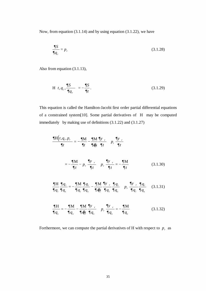
Now, from equation (3.1.14) and by using equation (3.1.22), we have

∂

∂ ρρ

Sq

p= (3.1.28)

Also from equation (3.1.13),

Η t qSq

Sti, ,

∂∂

∂∂ρ

= − . (3.1.29)

This equation is called the Hamilton-Jacobi first order partial differential equations

of a constrained system[10]. Some partial derivatives of H may be computed

immediately by making use of definitions (3.1.22) and (3.1.27)

( )∂

∂∂∂

∂∂

∂ψ

∂

∂ψ

∂ρ

ρ

ρρ

ρΗ Μ Μt q pt t q t

pt

i, ,&

= − − +

= − − + = −∂∂

∂ψ

∂

∂ψ

∂∂∂ρ

ρρ

ρΜ Μt

pt

pt t

(3.1.30)

∂∂

∂∂

∂∂

∂∂

∂∂

∂ψ

∂∂∂

∂ψ

∂∂∂σ σ σ

ρ

σρ

ρ

σ

Η Μ Μq

qq q

qq q q

qq

pq

qqi

i

i

i

i

i

i

i= − − +&

(3.1.31)

∂∂

∂∂

∂∂

∂ψ

∂

∂ψ

∂∂∂σ σ σ

ρ

σρ

ρ

σ σ

Η Μ Μ Μq q q q

pq q

= − − + = −&

(3.1.32)

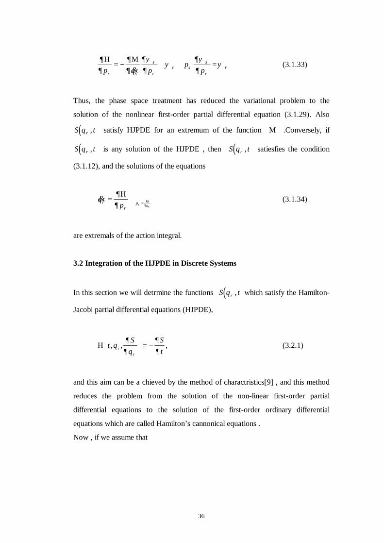
Forthermore, we can compute the partial derivatives of H with respect to pρ as

36

∂∂

∂∂

∂ψ∂

ψ∂ψ∂

ψρ σ

σ

ρρ σ

σ

ρρ

Η Μp q p

pp

= − + + =&

(3.1.33)

Thus, the phase space treatment has reduced the variational problem to the

solution of the nonlinear first-order partial differential equation (3.1.29). Also

( )S q tρ , satisfy HJPDE for an extremum of the function M .Conversely, if

( )S q tρ , is any solution of the HJPDE , then ( )S q tρ , satiesfies the condition

(3.1.12), and the solutions of the equations

&qpρ

ρ

∂∂

=Η

p Sqσ∂

∂ σ=

(3.1.34)

are extremals of the action integral.

3.2 Integration of the HJPDE in Discrete Systems

In this section we will detrmine the functions ( )S q tρ , which satisfy the Hamilton-

Jacobi partial differential equations (HJPDE),

Η t qS

qSti, ,

∂∂

∂∂ρ

= − , (3.2.1)

and this aim can be a chieved by the method of charactristics[9] , and this method

reduces the problem from the solution of the non-linear first-order partial

differential equations to the solution of the first-order ordinary differential

equations which are called Hamilton’s cannonical equations .

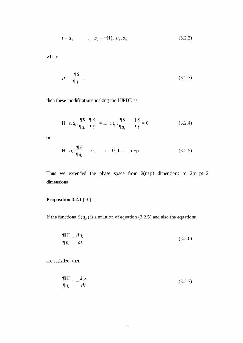
Now , if we assume that

37

( )t q p t q pi= = −0 0 0, , ,Η (3.2.2)

where

pS

qρρ

∂∂

= , (3.2.3)

then these modifications making the HJPDE as

′

=

+ =Η Ηt q S

qSt

t q Sq

Sti i, , , , ,∂

∂∂∂

∂∂

∂∂ρ ρ

0 (3.2.4)

or

′

=Η q

Sqr

r

,∂∂

0 , r = 0, 1,......, n+p (3.2.5)

Thus we extended the phase space from 2(n+p) dimensions to 2(n+p)+2

dimensions

Proposition 3.2.1 [10]

If the functions S q r( ) is a solution of equation (3.2.5) and also the equations

∂∂

′=

Ηp

d qdtr

r (3.2.6)

are satisfied, then

∂∂

′= −

Ηq

d pd tr

r (3.2.7)

38

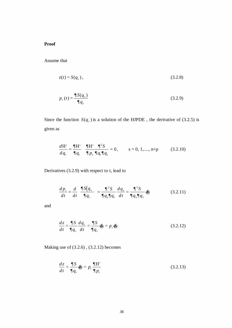
Proof

Assume that

z t S qr( ) ( )= , (3.2.8)

p tS q

qrs

r

( )( )

=∂

∂ (3.2.9)

Since the function S q r( ) is a solution of the HJPDE , the derivative of (3.2.5) is

given as

dd q q p

Sq qr r s r s

′=

′+

′=

Η Η Η∂∂

∂∂

∂∂ ∂

2

0, s = 0, 1,...., n+p (3.2.10)

Derivatives (3.2.9) with respect to t, lead to

( )d p

d tddt

S qq

Sq q

dqd t

Sq q

qr s

r s r

s

s rs=

= =

∂

∂∂

∂ ∂∂

∂ ∂

2 2

& (3.2.11)

and

d zd t

Sq

dqdt

Sq

q p qr

r

rr r r= = =

∂∂

∂∂

& & (3.2.12)

Making use of (3.2.6) , (3.2.12) becomes

d zd t

Sq

q ppr

r rr

= =′∂

∂∂∂

&Η (3.2.13)

39

Adding equations (3.2.11) and (3.2.10) we obtain

∂∂

∂∂

∂∂ ∂

∂∂ ∂

′+

′+ − =

Η Ηq p

Sq q

d pdt

Sq q

qr s r s

r

r ss

2 2

0&

& (3.2.14)

Using (3.2.6), (3.2.14) becomes

∂∂

∂∂ ∂

∂∂ ∂

′+ + − =

Ηq

qS

q qd pd t

Sq q

qr

sr s

r

r ss&

&&

2 2

0 , (3.2.15)

∂∂

′= −

Ηq

d pd tr

r . (3.2.16)

Also since

∂∂

∂∂ρ ρ

′=

Η Ηq q

, (3.2.17)

∂∂ ρ

ρΗq

d pdt

= − ρ =1,.....,n+p (3.2.18)

and

∂∂

∂∂

∂∂

′=

′= = −

Η Η Ηq t t

d pdt0

0 . (3.2.19)

Furthermore , we can obtain the last equation by the following way:

since ( )p t q pi0 = −Η , , ρ ,

40

d pd t

dd t t q

qp

p0 = − = − + +

Η Η Η Η∂∂

∂∂

∂∂ρ

ρρ

ρ& & (3.2.20)

By using (3.2.18), (3.2.20) becomes

d pd t t

0 = −∂∂Η

. (3.2.21)

In this theorem we extend the 2(n+p)-dimensional phase space in the equation

(3.2.1) to 2(n+p)+2 in the equation (3.2.5) by introducing t and H as generalized

co-ordinate and generalized momentum, respectively. Also, we can discuss that

&λ α is explicit independence of H, that is ,

∂∂

∂∂ λα α

′= =

+

Η Η& &qi

0 (3.2.22)

By using the equations (3.1.27) and (3.1.24), we have

∂∂ λα

α

Η& = − p ( )= − =G t q qi iα , , & 0

d pd t

d Gdt

α α= = 0, α = 1,.....,m (3.2.23)

This implies that ( )p G t q qi iα α= , , & are constants of motion .

Now the 2(n+p) first-order ordinary differential equations

41

∂∂

∂∂

ρρ

ρρ

ρ

′= −

′=

Η Ηq

pp

q& , & , =1,....,n+p (3.2.24)

are called Hamilton’s canonical equations[10] .

Now , the general solutions of the canonical equations are given as

( ) ( )q t u p t uρ ρ σ ρ ρ σξ η= =, , , (3.2.25)

where uσ are arbitrarily parameters .

More explicitly

( ) ( ) ( )

( ) ( ) ( ) ( )

q t u q t u p t u

p t u t t u q p t u t

i i i i= = = =

= = = = = −

ξ λ ξ η

η ξ η ξ η

σ α α α σ σ

α α σ σ σ ρ ρ

, , , , ,

, , , , , , ,0 0 0 0 Η

(3.2.26)

Integration of (3.2.12) gives us the Hamilton’s principal function [6], [10]

( )S q tρ , in terms of arbitrary parameters uσ ,

( ) ( )z t t u s u

q pprr r

ru

t

( ) , ( ),

( )

= = + ∫σ η∂

∂ρ ρτ ρ

Η q

pr rr r

d t==ξη

(3.2.27)

with initial values

σ τρ ρ= =s u t u( ) , ( ) . (3.2.28)

42

CHAPTER IV

HAMILTON-JACOBI THEORY OF CONTENUOUS SYSTEMS

In this chapter we will study the construction of the Hamilton-Jacobi partial

differential equation for classical field systems, or continuous systems in 5n-

dimensional phase space and the integration of it by the method of characteristics.

The motivation behind this chapter is to establish a valid Hamiltonian approach of

classical field such that the passage from the Lagrangian to the Hamiltonian

approach follows naturally and the Hamilton-Jacobi partial differential equation

plays the fundamental role in this study.

We say that the dynamical system is continuous if between every two points in the

system there exist a point. For example, if a particle moves on the surface, the

particle will be passing at every point on the surface.

4.1 Determination of the Hamilton-Jacobi Partial Differential Equation

(HJPDE) for Continuous Systems

In this section we will construct the Hamilton-Jacobi partial differential equation

(HJPDE) by using the continuous indices x,y,z[4].

If Q is the configuration manifold, that means the generalized co-ordinates

q i belongs to Q and if we defined the Lagrangian ( )L L q q ti i= , & , is the mapping

from the tangent bundle[12] TQ to R, i.e.

L TQ R: → , (4.1.1)

then we say that the curve qi=qi(t) are extremals [4], [10], [11], [14] of the action

integral

( )Ι = ∫ L q q t dti it

t

, & ,0

1

, (4.1.2)

43

if the Euler-Lagrange equations

ddt

Lq

Lq

ii i

∂∂

∂∂&

− = ∀0 (4.1.3)

are valid under the condition that there is no variation at t and t0 1 . Also, we

define the Euler-Lagrange equations under transformation

( )L L L q q tdF q t

d ti ii→ ′ = −, & ,

( , ) (4.1.4)

where F is an arbitrary at least twice-differentiable function. In the continuous

systems, the equivalent Lagrangian density is defined as

′ℑ = ℑ −d S x

d xiµ ν

µ

ϕ( , ), µ ν, , , ,= 1 2 3 4 (4.1.5)

where ℑ = ℑ

ϕ ∂ϕ∂ µ

νii

x x, , is the Lagrangian density defined on the tangent

bundle of the manifold of field ϕ νi x( ) , and the arbitrary four functions Sµ are at

least twice differentiable .

Proposition 4.1.1

Consider a regular Lagrangian density[4], [14] ′ℑ

ϕ ∂ϕ∂ µ

νii

x x, , . If it is

possible to determine a set of differentiable functions η ϕµ νi i x( , ) and four

functions S xiµ νϕ( , ) such that

a) ( )′ℑ ϕ ηµ νi i x, , =0, (4.1.6)

44

b) ′ℑ > 0 in the neighborhood of the point with co-ordinates η µ i ,

then the solutions of the system of partial differential equations

∂ϕ∂

ηµ

µi

ix= (4.1.7)

are extremals of the action integral

Ι = ℑ

∫ ϕ ∂ϕ

∂ µµ

νi

ix x d x, , 4 (4.1.8)

if all the variations at the boundary are zero. The solutions of the equation

(4.1.7)are extremals of the action integral (4.1.8) as well if the following equations

hold:

( )∂

∂ϕ η

∂

∂ϕηµ

µµ ν

µµ

Sx

xS

i ii

i= ℑ −, , , (4.1.9)

and

∂

∂∂ϕ∂ ν

ℑ

i

x

∂ϕ∂

η

µ

µµ

∂

∂ϕijx i

S=

= (4.1.10)

Proof

Let ℑ′ be a function of variables ∂ϕi/∂xµ , then conditions a) and b) say that ℑ′

has a local minimum at the point ∂ϕ∂

ηµ

µi

ix= , ∀µ, i and it is minimum value at

45

that point is zero. But since equation (4.1.5) is satisfied, ℑ is a local minimum at

ηµi and also the solution of ∂ϕ∂

ηµ

µi

ix= are extremals of the action integral (4.1.8) .

Now from the conditions a) and b), the solutions of equation (4.1.7) are

extremals of the action integral, this implies

′ℑ = ℑ −d S x

d xiµ ν

µ

ϕ( , )= 0 (4.1.11)

or more explicitly

( )ℑ − − =ϕ η∂

∂ϕη

∂

∂µ νµ

µµ

µi i

iix

S Sx

, , 0 (4.1.12)

and this implies

( )ℑ − =ϕ η∂

∂ϕη

∂

∂µ νµ

µµ

µi i

iix

S Sx

, , (4.1.13)

Since ′ℑ is minimum at ηµ i and equals zero at this point,

∂

∂∂ϕ∂ ν

ℑ

i

x

∂ϕ

∂η

µµ

jjx

== ∂

∂∂ϕ∂ ν

ℑ

i

x

∂ϕ

∂η

µ

µµ

∂

∂ϕjjx i

S=

− = 0 (4.1.14)

and equation the (4.1.10) is hold .

46

Definition 4.1.1

If ℑ

ϕ ∂ϕ

∂ ννi

ix x, , is a regular Lagrangian density[8], the generalized

momentum Ρµ i is defined as

Ρµ

µ

∂

∂∂ϕ∂

i

i

x

=ℑ

(4.1.15)

since ℑ is regular, we can solve equation (4.1.15) ∂ϕi/∂xµ in terms of

Ρν νϕi i and x, , i.e.

( )∂ϕ∂

ξ ϕµ

µ ν νi

i i jxx= Ρ , , (4.1.16)

When using equations (4.1.15) and (4.1.16), the equation (4.1.9) leads to

( )ℑ − =ϕ ξ ξ∂

∂µ ν µ µµ

µi i i ix

Sx

, , Ρ (4.1.17)

Definition 4.1.2

The Hamiltonian density H of classical field systems is defined on Τ ∗ Q [13] as

( ) ( )H x xi i i i i iϕ ϕ ξ ξµ ν µ ν µ µ, , , ,Ρ Ρ= −ℑ + (4.1.18)

Using (4.1.17) and (4.1.18) the Hamilton-Jacobi equation of a continuous system

will be

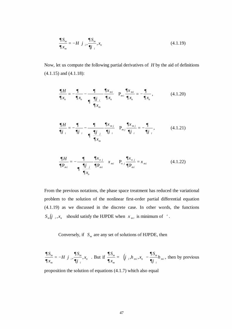
47

∂

∂ϕ

∂

∂ϕµ

µ

µν

Sx

HS

xii

= −

, , (4.1.19)

Now, let us compute the following partial derivatives of H by the aid of definitions

(4.1.15) and (4.1.18):

∂∂

∂∂

∂

∂∂ϕ∂

∂ξ

∂

∂ξ

∂∂∂ν ν

µ

µ

νµ

µ

ν ν

Hx x

xx x x

i

ii

i= −ℑ

−ℑ

+ = −ℑ

Ρ , (4.1.20)

∂∂ϕ

∂∂ϕ

∂

∂∂ϕ

∂

∂ξ

∂ϕ

∂ξ

∂ϕ∂∂ϕ

µ

µµ

µH

xi i j

j

ij

j

i i

= −ℑ

−ℑ

+ = −ℑ

Ρ , (4.1.21)

∂∂

∂

∂∂ϕ

∂

∂ξ

∂ξ

∂ξ

∂ξ

µ

ν

ν

µµ ν

ν

µµ

H

xi j

j

ii j

j

iiΡ Ρ

ΡΡ

= −ℑ

+ + = (4.1.22)

From the previous notations, the phase space treatment has reduced the variational

problem to the solution of the nonlinear first-order partial differential equation

(4.1.19) as we discussed in the discrete case. In other words, the functions

( )S xiµ νϕ , should satisfy the HJPDE when ξ µ i is minimum of ′ℑ .

Conversely, if Sµ are any set of solutions of HJPDE, then

∂

∂ϕ

∂

∂ϕµ

µ

µν

Sx

HS

xii

= −

, , . But if ( )∂

∂ϕ η

∂

∂ϕηµ

µµ ν

µµ

Sx

xS

i ii

i= ℑ −, , , then by previous

proposition the solution of equations (4.1.7) which also equal

48

∂ϕ∂

∂∂µ µ

i

ixH

=Ρ

Ρν

ν∂∂ ϕj

j

S=

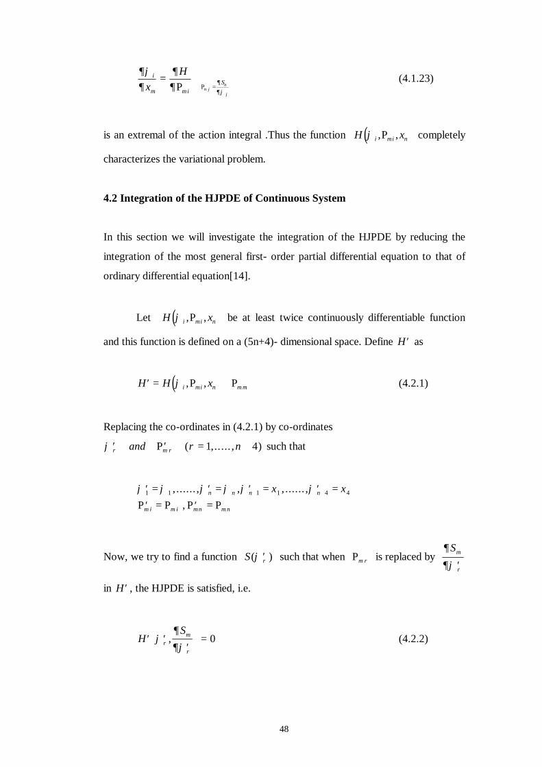
(4.1.23)

is an extremal of the action integral .Thus the function ( )H xi iϕ µ ν, ,Ρ completely

characterizes the variational problem.

4.2 Integration of the HJPDE of Continuous System

In this section we will investigate the integration of the HJPDE by reducing the

integration of the most general first- order partial differential equation to that of

ordinary differential equation[14].

Let ( )H xi iϕ µ ν, ,Ρ be at least twice continuously differentiable function

and this function is defined on a (5n+4)- dimensional space. Define ′H as

( )′ = +H H xi iϕ µ ν µ µ, ,Ρ Ρ (4.2.1)

Replacing the co-ordinates in (4.2.1) by co-ordinates

′ ′ = +ϕ ρρ µ ρand nΡ ( ,..... , )1 4 such that

′ = ′ = ′ = ′ =′ = ′ =

+ +ϕ ϕ ϕ ϕ ϕ ϕ

µ µ µ ν µ ν

1 1 1 1 4 4, ...... , , , ...... ,,

n n n n

i i

x xΡ Ρ Ρ Ρ

Now, we try to find a function S( )′ϕ ρ such that when Ρµ ρ is replaced by ∂

∂ϕµ

ρ

S′

in ′H , the HJPDE is satisfied, i.e.

′ ′′

=H

Sϕ

∂

∂ϕρµ

ρ

, 0 (4.2.2)

49

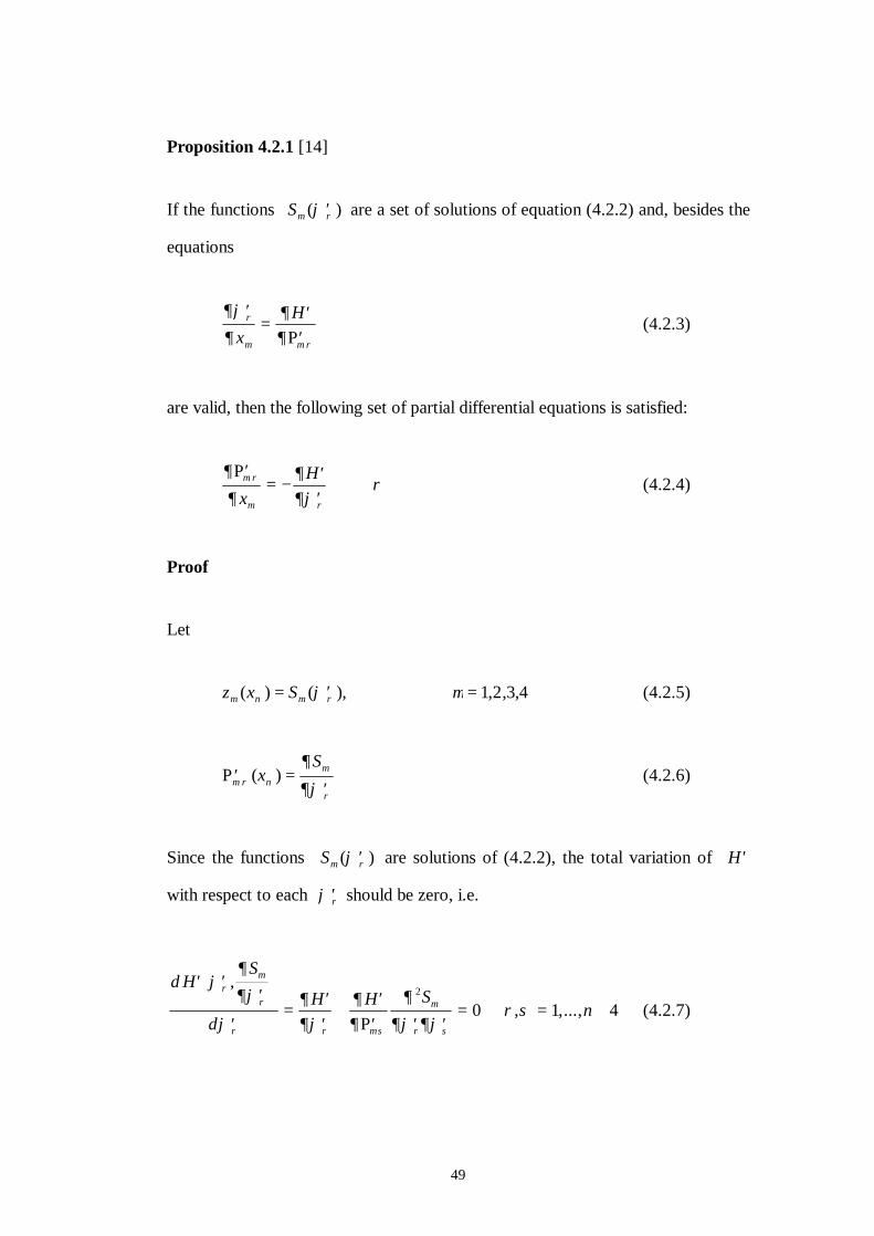
Proposition 4.2.1 [14]

If the functions Sµ ρϕ( )′ are a set of solutions of equation (4.2.2) and, besides the

equations

∂ϕ

∂∂∂

ρ

µ µ ρ

′=

′′x

HΡ

(4.2.3)

are valid, then the following set of partial differential equations is satisfied:

∂

∂∂∂ϕ

ρµ ρ

µ ρ

′= −

′′

∀Ρ

xH (4.2.4)

Proof

Let

z x Sµ ν µ ρϕ µ( ) ( ), , , ,= ′ = 1 2 3 4 (4.2.5)

′ =′

Ρµ ρ νµ

ρ

∂

∂ϕ( )x

S (4.2.6)

Since the functions Sµ ρϕ( )′ are solutions of (4.2.2), the total variation of ′H

with respect to each ′ϕ ρ should be zero, i.e.

d HS

dH H S

n′ ′

′

′=

′′

+′

′ ′ ′= ∀ = +

ϕ∂

∂ϕ

ϕ∂∂ϕ

∂∂

∂

∂ϕ ∂ϕρ σ

ρµ

ρ

ρ ρ µ σ

µ

ρ σ

,, ,...,

Ρ

2

0 1 4 (4.2.7)

50

Also since (4.2.5) is valid,

( )∂

∂

∂ ϕ

∂

∂

∂ϕ

∂ϕ

∂µ

ν

µ ρ

ν

µ

ρ

ρ

ν

zx

Sx

Sx

=′

=′

′( ) (4.2.8)

From (4.2.3) and (4.2.6), (4.2.8) becomes

∂

∂

∂

∂ϕ

∂ϕ

∂∂∂

∂∂

µ

ν

µ

ρ

ρ

νµ ρ

ν ρµ ν µ

ν

zx

Sx

H Hi

i

=′

′= ′

′′

= +ΡΡ

Ρ ΡΡ

(4.2.9)

Partial derivative of (4.2.6) with respect to xµ gives us

∂

∂

∂

∂ϕ ∂ϕ∂ϕ∂

µ ρ

µ

µ

ρ σ

σ

µ

′=

′ ′′Ρ

xS

x

2

(4.2.10)

Adding equations (4.2.7) and (4.2.10), and using (4.2.3), we have

∂∂ϕ

∂

∂

∂

∂ϕ ∂ϕ∂ϕ∂

∂∂ρ

µ ρ

µ

µ

ρ σ

σ

µ µ σ

′′

+′

=′ ′

′−

′′

=

Hx

Sx

HΡ

Ρ

2

0 (4.2.11)

Equation (4.2.11) leads to

∂∂ϕ

∂

∂ρ

µ ρ

µ

′′

= −′H

xΡ

(4.2.12)

Using equations (4.2.1), one may writes another form of HJPDE as

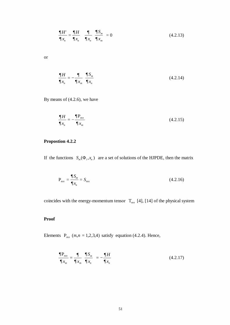
51

∂∂

∂∂

∂∂

∂

∂ν ν ν

µ

µ

′= +

Hx

Hx x

Sx

= 0 (4.2.13)

or

∂∂

∂∂

∂

∂ν µ

µ

ν

Hx x

Sx

= −

(4.2.14)

By means of (4.2.6), we have

∂∂

∂

∂ν

µ ν

µ

Hx x

= −Ρ

(4.2.15)

Propostion 4.2.2

If the functions S xiµ ν( , )Φ are a set of solutions of the HJPDE, then the matrix

Ρµ νµ

νµ ν

∂

∂= =

Sx

S (4.2.16)

coincides with the energy-momentum tensor Τµ ν [4], [14] of the physical system

Proof

Elements Ρµ ν µ ν( , , , , )= 1 2 3 4 satisfy equation (4.2.4). Hence,

∂

∂∂

∂

∂

∂∂∂

µ ν

µ µ

µ

ν ν

Ρ

x xSx

Hx

=

= − (4.2.17)

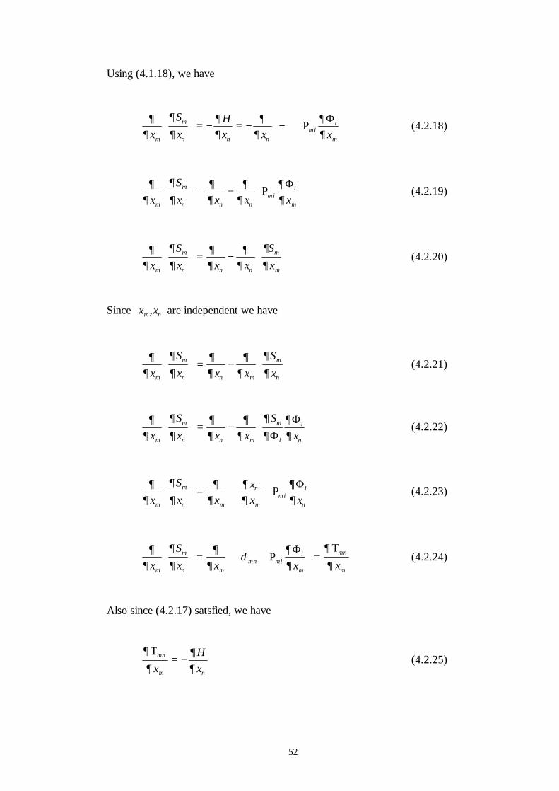
52

Using (4.1.18), we have

∂∂

∂

∂∂∂

∂∂

∂∂µ

µ

ν ν νµ

µxSx

Hx x xi

i

= − = − −ℑ +

Ρ

Φ (4.2.18)

∂∂

∂

∂∂∂

∂∂

∂∂µ

µ

ν ν νµ

µxSx x x xi

i

=

ℑ−

Ρ

Φ (4.2.19)

∂∂

∂

∂∂∂

∂∂

∂

∂µ

µ

ν ν ν

µ

µxSx x x

Sx

=

ℑ−

(4.2.20)

Since x xµ ν, are independent we have

∂∂

∂

∂∂∂

∂∂

∂

∂µ

µ

ν ν µ

µ

νxSx x x

Sx

=

ℑ−

(4.2.21)

∂∂

∂

∂∂∂

∂∂

∂

∂∂∂µ

µ

ν ν µ

µ

νxSx x x

Sxi

i

=

ℑ−

ΦΦ (4.2.22)

∂∂

∂

∂∂

∂∂∂

∂∂µ

µ

ν µ

ν

µµ

νxSx x

xx xi

i

= ℑ +

Ρ

Φ (4.2.23)

∂∂

∂

∂∂

∂δ

∂∂

∂

∂µ

µ

ν µµ ν µ

µ

µ ν

µxSx x x xi

i

= ℑ +

=Ρ

Φ Τ (4.2.24)

Also since (4.2.17) satsfied, we have

∂

∂∂∂

µ ν

µ ν

Τ

xHx

= − (4.2.25)

53

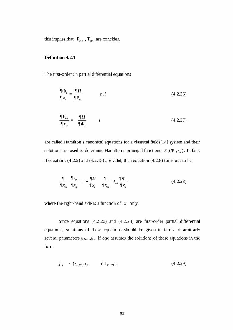
this implies that Ρ Τµ ν µ ν, are concides.

Definition 4.2.1

The first-order 5n partial differential equations

∂∂

∂∂

µµ µ

ΦΡ

i

ixH i= ∀ , (4.2.26)

∂

∂∂∂

µ ι

µ ι

Ρ

ΦxH i= − ∀ (4.2.27)

are called Hamilton’s canonical equations for a classical fields[14] system and their

solutions are used to determine Hamilton’s principal functions S xiµ ν( , )Φ . In fact,

if equations (4.2.5) and (4.2.15) are valid, then equation (4.2.8) turns out to be

∂∂

∂

∂∂∂

∂∂

∂∂µ

µ

ν ν µµ

νxzx

Hx x xi

i

= − +

Ρ

Φ (4.2.28)

where the right-hand side is a function of xν only.

Since equations (4.2.26) and (4.2.28) are first-order partial differential

equations, solutions of these equations should be given in terms of arbitrarly

several parameters u1,...,uk. If one assumes the solutions of these equations in the

form

ϕ ξ νi i jx u= ( , ) , i=1,....,n (4.2.29)

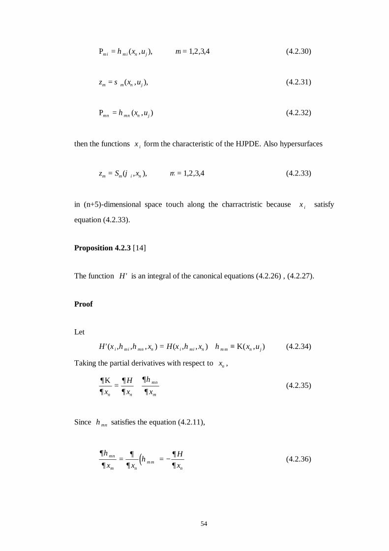
54

Ρµ µ νη µi i jx u= =( , ), , , ,1 2 3 4 (4.2.30)

z x u jµ µ νσ= ( , ), (4.2.31)

Ρµ ν µ ν νη= ( , )x u j (4.2.32)

then the functions ξ i form the characteristic of the HJPDE. Also hypersurfaces

z S xiµ µ νϕ µ= =( , ), , , ,1 2 3 4 (4.2.33)

in (n+5)-dimensional space touch along the charractristic because ξ i satisfy

equation (4.2.33).

Proposition 4.2.3 [14]

The function ′H is an integral of the canonical equations (4.2.26) , (4.2.27).

Proof

Let

′ = + ≡H x H x x ui i i i j( , , , ) ( , , ) ( , )ξ η η ξ η ηµ µ ν ν µ ν µ µ νΚ (4.2.34)

Taking the partial derivatives with respect to xν ,

∂∂

∂∂

∂η

∂ν ν

µ ν

µ

Κx

Hx x

= + (4.2.35)

Since ηµ ν satisfies the equation (4.2.11),

( )∂η

∂∂

∂η

∂∂

µ ν

µ νµ µ

νx xHx

= = − (4.2.36)

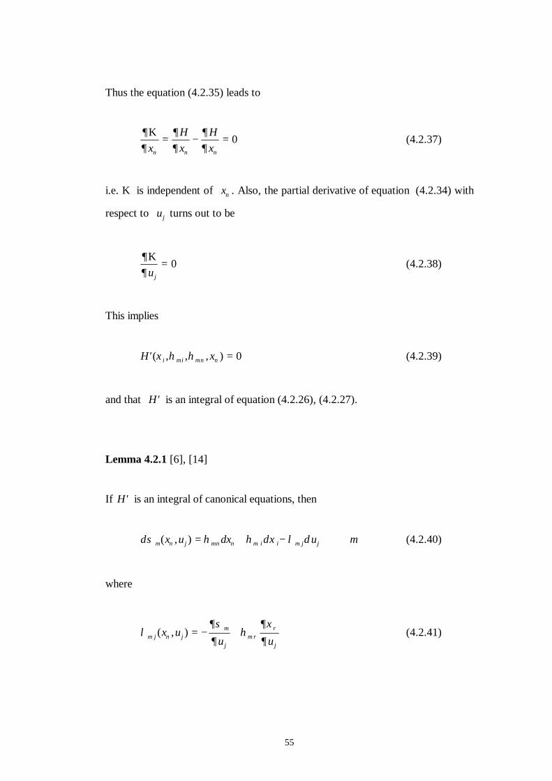
55

Thus the equation (4.2.35) leads to

∂∂

∂∂

∂∂ν ν ν

Κx

Hx

Hx

= − = 0 (4.2.37)

i.e. K is independent of xν . Also, the partial derivative of equation (4.2.34) with

respect to u j turns out to be

∂∂

Κu j

= 0 (4.2.38)

This implies

′ =H xi i( , , , )ξ η ηµ µ ν ν 0 (4.2.39)

and that ′H is an integral of equation (4.2.26), (4.2.27).

Lemma 4.2.1 [6], [14]

If ′H is an integral of canonical equations, then

d x u dx d d uj i i j jσ η η ξ λ µµ ν µ ν ν µ µ( , ) = + − ∀ (4.2.40)

where

λ∂σ

∂η

∂ξ

∂µ νµ

µ ρρ

j jj j

x uu u

( , ) = − + (4.2.41)

56

Proof

If equation (4.2.39) is valid, then

d Kdu

Hu

Hu

Hz uj j j j

=′

+′

′+

′=

∂∂

∂ξ

∂∂∂

∂η

∂∂∂

∂σ

∂ρ

ρ

µ ρ

µ ρ

µ

µ

Φ Ρ0 (4.2.42)

Now with the help of equations (4.2.3) and (4.2.4), we obtain

∂∂

∂ξ

∂µ ρ

ρ

µ

′′

=H

xΡ, (4.2.43)

and

∂∂

∂∂

∂∂

∂∂

∂

∂ρ ρ µ

µ

ρ

′′

=′

′+

′′

H H Hz

S

i

i

Φ ΦΦΦ Φ

(4.2.44)

∂∂

∂∂

∂∂

∂

∂ρ ρ µ

µ

ρ

′′

=′′

+′

′H H H

zS

Φ Φ Φ (4.2.45)

∂∂

∂η

∂∂∂

ηρ

µ ρ

µ µµ ρ

′′

= − +′H

xHzΦ

(4.2.46)

also ∂∂

∂∂µ µ

′=

Hz

Hz

, equation (4.2.42) leads to

d Kdu x u x u

Hz u uj j j j j

= − + − +

=

∂η

∂

∂ξ

∂

∂ξ

∂

∂η

∂∂∂

∂σ

∂η

∂ξ

∂µ ρ

µ

ρ ρ

µ

µ ρ

µ

µµ ρ

ρ 0 (4.2.47)

From the equation (4.2.8)

57

∂σ

∂η

∂ξ

∂µ

µµ ρ

ρ

µx x= (4.2.48)

Thus

∂ σ

∂ ∂∂

∂η

∂ξ

∂

∂η

∂

∂ξ

∂

∂ ξ

∂ ∂ηµ

µµ ρ

ρ

µ

µ ρ ρ

µ

ρ

µµ ρ

2 2

x u u x u x u xj j j j

=

= + (4.2.49)

since ∂ ξ

∂ ∂η

∂∂

η∂ξ

∂

∂η

∂

∂ξ

∂ρ

µµ ρ

µµ ρ

ρ µ ρ

µ

ρ2

u x x u x uj j j

=

− ,

∂ σ

∂ ∂

∂η

∂

∂ξ

∂∂

∂η

∂ξ

∂

∂η

∂

∂ξ

∂µ

µ

µ ρ ρ

µ µµ ρ

ρ µ ρ

µ

ρ2

x u u x x u x uj j j j

= +

− (4.2.50)

∂ σ

∂ ∂∂

∂η

∂ξ

∂

∂η

∂

∂ξ

∂

∂η

∂

∂ξ

∂µ

µ µµ ρ

ρ µ ρ

µ

ρ µ ρ ρ

µ

2

x u x u x u u xj j j j

=

= − + (4.2.51)

∂∂

∂σ

∂η

∂ξ

∂

∂η

∂

∂ξ

∂

∂η

∂

∂ξ

∂µ

µµ ρ

ρ µ ρ

µ

ρ µ ρ ρ

µx u u x u u xj j j j

−

= − + (4.2.52)

Inserting the right-hand side of the equation (4.2.52) in the equation (4.2.47), one

obtains

∂ λ

∂∂∂

λµ

µ µµ

jjx

Hz

− = 0 (4.2.53)

since σ σµ µ ν= ( , )x u j ,

58

dx

dxu

duj

jσ∂σ

∂

∂σ

∂µµ

νν

µ= + (4.2.54)

From the definition (4.2.41), and the equation (4.2.48), the equation (4.2.54) leads

to

dx

dxu

dujj

jσ η∂ξ

∂λ η

∂ξ

∂µ µ ρρ

νν µ µ ρ

ρ= + − +

(4.2.55)

The variation of ξ ξρ ρ ν= ( , )x u j gives dx

dxu

duj

jξ∂ξ

∂

∂ξ

∂ρρ

νν

ρ= + , and the

equation (4.2.55) leads to

dx

dxu

du du d duj

j j j j jσ η∂ξ

∂

∂ξ

∂λ η ξ λµ µ ρ

ρ

νν

ρµ µ ρ ρ µ= +

− = − (4.2.56)

or explicitly.

d d dx dui i j jσ η ξ η λµ µ µ ν ν µ= + − (4.2.57)

let us parametrize the initial values by arbitrary function τ ν ( )u j as

x ujν ντ0 = ( ) (4.2.58)

and define the initial values of Φ Ρi and, µ ρ µσ as

ξ ρ ν ρ( , ) ( ),x u uj j0 ≡ Α (4.2.59)

ηµ ρ ν µ ρ( , ) ( ),x u uj j0 ≡ Β (4.2.60)

59

σ µ ν µ( , ) ( ).x u s uj j0 ≡ (4.2.61)

Lemma 4.2.2 [6], [14]

The functions λ µ j are independent of xν , i.e.

λ λµ ν µ νj i j ix u x u( , ) ( , )= 0 (4.2.62)

Proof

Consider the partial derivatives of (4.2.61) with respect to u j

− − = − ∀∂σ

∂∂τ∂

∂σ

∂

∂

∂µµ

ν

ν µ µ

x u usu

jj j j

, (4.2.63)

Also, consider the partial derivatives of (4.2.59) with respect to u j

∂ξ

∂∂τ∂

∂ξ

∂

∂

∂ρ

ν

ν ρ ρ

x u u uj j j

+ =Α

(4.2.64)

Multiplying equation (4.2.64) with ηµ ρ , one obtains

η∂ξ

∂∂τ∂

η∂ξ

∂

∂

∂µ ρρ

ν

νµ ρ

ρµ ρ

ρ

x u u uj j j

+ = ΒΑ

(4.2.65)

Adding equations (4.2.63) and (4.2.65) and noticing that equation (4.2.48) is valid,

one arrives at the result

60

− + = − + =∂

∂

∂

∂

∂σ

∂η

∂ξ

∂λµ

µ ρρ µ

µ ρρ

µ

su u u uj j j j

jΒΑ

(4.2.66)

This means that λ µ j are independent of xν .

Lemma 4.2.3 [14]

The initial total differential d x u jσ µ ν( , )0 is

d x u d x u s u dj j jσ σµ ν ν µ µ ρ ρ( , ) [ ( , ) ( )]0 = − + Β Α (4.2.67)

Proof

By replacing λ µ j in the equation (4.2.66) by its value in the equation (4.2.56), we

have

d x u d du dsu

d uu

d uj j jj

jj

jσ η ξ λ η ξ∂

∂

∂

∂µ ν µ ρ ρ µ µ ρ ρµ

µ ρρ( , ) = − = + − Β

Α(4.2.68)

d x u ds d d d x uj jσ η ξ σµ ν µ µ ρ ρ µ ρ ρ µ ν( , ) ( , )− + = =Β Α 0 (4.2.69)

At this step one may arrange the prescribed initial values

Α Βρ µ ρ µ( ) , ( ) ( )u u and s uj j j in such a way that the left-hand side of equation

(4.2.66) is zero. Hence all functions λµj(xν,ui) will be set to zero. For the sake of

simplicity, assume that the functions s u and uj i jµ ( ) ( )Α are given. The problem

now is to calculate the functions Βµ ρ µ νλ µ( ) ( , ) ,u such that x u jj j i0 0= ∀ .

Lemma 4.2.4 [6], [14]

61

For given functions s u jµ ( ) and Αρ ( )u j the set of equations

λ∂

∂

∂

∂µµ ν

µµ ρ

ρj j

j j

x usu u

j( , ) ,0 0= − + = ∀ΒΑ

(4.2.70)

can be solved for the functions Βµ ρ ( )uj if

∂ξ∂

i

ju≠ 0 (4.2.71)

Proof

The explicit form of equation (4.2.66) is

− + + =∂

∂∂∂

∂τ∂

µµ µ ν

νsu u

Cuj

ii

j j

ΒΑ 0 (4.2.72)

where the functions C u jµ ν ( ) are the initial values of Ρµ ν , i.e.

Ρµ ν ν µ ν( , ) ( )x u C uj j0 = (4.2.73)

In this case, the equation (4.2.1) can be written as

H x C Hi i( , , )ν µ µ µη ξ0 0+ = = ′ (4.2.74)

By using the implicit function theorem , which states that one can solve the set of

equations (4.2.72) for Βµ i if the following condition holds:

62

∂∂

∂

∂∂∂

∂τ∂

∂∂

∂

∂∂τ∂µ

µµ µ ν

ν µ ν

µ

ν

ΒΒ

Α ΑΒi j

ii

j j

i

j i j

su u

Cu u

Cu

− + −

= + ≠ 0 (4.2.75)

where Cµ ν are not independent of Βµ i but

∂

∂η

∂

∂∂∂η

µ ν

µ

µ ν

µ

C CH

H

i i

=′

′ (4.2.76)

By using (4.2.74), we have

δ∂

∂ηδ

∂∂ηµ ν

µ µ

µµ ν

µ

C H

i i

= − (4.2.77)

∂

∂ηδ

∂∂η

∂∂η

µ ν

µµ ν

µ ν

C H H

i i i

= − = − (4.2.78)

The equation (4.2.76) becomes

∂

∂η

∂

∂∂∂η

µ ν

µ

µ ν

µ

C CH

H

i i

=′

′= − = −δ

∂∂η

∂∂ηµ ν

µ ν

H H

i i

(4.2.79)

Thus the determinant (4.2.75) reads as

∂∂

∂∂η

∂τ∂ν

νΑi

j i juH

u− ≠ 0 (4.2.80)

since ξ τν ν νi j i j jx u u x u( , ) ( ) , ( ),0 0= =Α

63

∂ξ∂

∂∂

∂ξ∂

∂τ∂ν

νi

j

i

j

i

ju u x u= −

Α (4.2.81)

and from equation (4.2.26), we have

∂ξ∂

∂∂ην ν

i

ixH

= . (4.2.82)

Then

∂ξ∂

∂∂

∂ξ∂

∂τ∂ν

νi

j

i

j

i

ju u x u= −

Α= −

∂∂

∂∂η

∂τ∂ν

νΑi

j i juH

u (4.2.83)

Condition (4.2.80) takes the form

∂ξ∂

i

ju≠ 0 i, j =1,.....,n. (4.2.84)

As a conclusion, if we choose those characteristics for which the condition

(4.2.71) is valid, then it is always possible from the last lemma to set all functions

λ µ νj ix u( , ) to be zero such that the total differential reads as

d x u dx dj i iσ η η ξµ ν µ ν ν µ( , ) = + (4.2.85)

ensuring that

Ρ Ρµ νµ

νµ

µ∂

∂

∂

∂ϕ= =

Sx

Si

i

, . (4.2.86)

Lemma 4.2.5 [14]

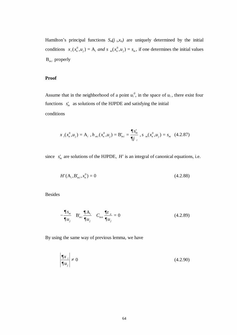
64

Hamilton’s principal functions Sµ(ϕi,xν) are uniquely determined by the initial

conditions ξ σν µ ν µi j i jx u and x u s( , ) ( , )0 0= =Α , if one determines the initial values

Βµ i properly

Proof

Assume that in the neighborhood of a point ui0, in the space of ui , there exist four

functions ′sµ as solutions of the HJPDE and satisfying the initial

conditions

ξ η∂

∂ϕσν µ ν µ

µµ ν µi j i i j i

ijx u x u

sx u s( , ) , ( , ) , ( , )0 0 0= = ′ =

′=Α Β (4.2.87)

since ′sµ are solutions of the HJPDE, ′H is an integral of canonical equations, i.e.

′ ′ =H xi i( , , )Α Βµ ν0 0 (4.2.88)

Besides

− + ′ + =∂

∂∂∂

∂τ∂

µµ µ ν

νsu u

Cuj

ii

j j

ΒΑ 0 (4.2.89)

By using the same way of previous lemma, we have

∂ξ∂

i

ju≠ 0 (4.2.90)

65

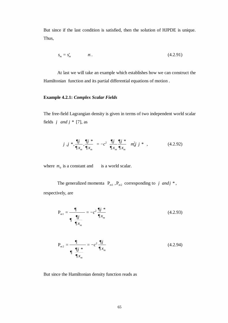
But since if the last condition is satisfied, then the solution of HJPDE is unique.

Thus,

s sµ µ µ= ′ ∀ . (4.2.91)

At last we will take an example which establishes how we can construct the

Hamiltonian function and its partial differential equations of motion .

Example 4.2.1: Complex Scalar Fields

The free-field Lagrangian density is given in terms of two independent world scalar

fields ϕ ϕand ∗ [7], as

ℑ ∗∗

= −

∗+ ∗

ϕ ϕ

∂ϕ∂

∂ϕ∂

∂ϕ∂

∂ϕ∂

µ ϕϕµ µ µ µ

, , ,x x

cx x

202 , (4.2.92)

where µ 0 is a constant and ℑ is a world scalar.

The generalized momenta Ρ Ρµ µ1 2, corresponding to ϕ ϕand ∗ ,

respectively, are

Ρµ

µ

µ

∂

∂∂ϕ∂

∂ϕ∂1

2=ℑ

= −∗

x

cx

(4.2.93)

Ρµ

µ

µ

∂

∂∂ϕ∂

∂ϕ∂2

2=ℑ

∗

= −

x

cx

(4.2.94)

But since the Hamiltonian density function reads as

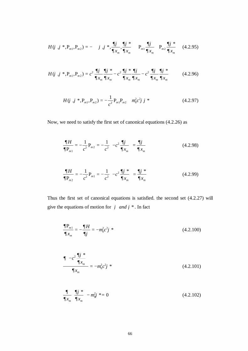
66

Hx x x x

( , , , ) , , ,ϕ ϕ ϕ ϕ∂ϕ∂

∂ϕ∂

∂ϕ∂

∂ϕ∂µ µ

µ µµ

µµ

µ

∗ = −ℑ ∗∗

+ +

∗Ρ Ρ Ρ Ρ1 2 1 2 (4.2.95)

H cx x

cx x

cx x

( , , , )ϕ ϕ∂ϕ∂

∂ϕ∂

∂ϕ∂

∂ϕ∂

∂ϕ∂

∂ϕ∂µ µ

µ µ µ µ µ µ

∗ =∗

−∗

−∗

Ρ Ρ1 22 2 2 (4.2.96)

Hc

c( , , , )ϕ ϕ µ ϕϕµ µ µ µ∗ = − + ∗Ρ Ρ Ρ Ρ1 2 2 1 2 02 21 (4.2.97)

Now, we need to satisfy the first set of canonical equations (4.2.26) as

∂∂

∂ϕ∂

∂ϕ∂µ

µµ µ

Hc c

cx xΡ

Ρ1

2 2 221 1

= − = − −

= (4.2.98)

∂∂

∂ϕ∂

∂ϕ∂µ

µµ µ

Hc c

cx xΡ

Ρ2

2 1 221 1

= − = − −∗

=

∗ (4.2.99)

Thus the first set of canonical equations is satisfied. the second set (4.2.27) will

give the equations of motion for ϕ ϕand ∗ . In fact

∂

∂∂∂ϕ

µ ϕµ

µ

Ρ 102 2

xH c= − = − ∗ (4.2.100)

∂

∂ϕ∂

∂µ ϕµ

µ

−∗

= − ∗

cx

xc

2

02 2 (4.2.101)

∂∂

∂ϕ∂

µ ϕµ µx x

∗

− ∗=0

2 0 (4.2.102)

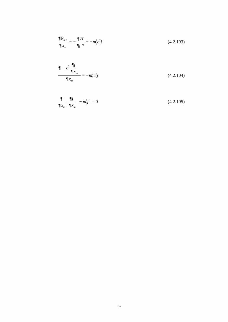
67

∂

∂∂∂ϕ

µ ϕµ

µ

Ρ 202 2

xH c= −∗

= − (4.2.103)

∂

∂ϕ∂

∂µ ϕµ

µ

−

= −

cx

xc

2

02 2 (4.2.104)

∂∂

∂ϕ∂

µ ϕµ µx x

− =0

2 0 (4.2.105)

68

CHAPTER V

CONCLUSION

The importance of partial differential equations clearly appears in many physical

problems. If we can solve such differential equations, we will be able find out the

equations of motion of physical system.

The solution of the partial differential equation is more complicated than

the solution of the ordinary differential equation. As shown in chapter two, we

could simplify the problem. We proved that every solution of a system of partial

differential equations of the form

∂∂

∂∂α

α β

Ft

b t x Fxi j

i

+ =( , ) 0 , α =1,.....,m (5.1)

is an integral of the total differential equations in the form

d x b t x d ti i j= α β α( , ) (5.2)

We also found out the integrability conditions of the total differential equations

(5.2).

A canonical formulation of singular system leads to equations of motion.

These equations of motion are total differential equations of the type (5.2). The

construction and integration of the equations of motion of singular system are

discussed. The equations of motion of a singular system with constraints are

integrable if the variation of these constraints is identically zero. This method needs

more elaboration in future work.

69

In chapter three, Caratheodory’s equivalent Lagrangians method is used to

construct the Hamilton-Jacbi formulation of a regular constrained system. This

method allows us to treat the variational problem as the problem of minimization

undetermined multipliers λα as generalized velocities makes it possible to define

the constraint functions as the generalized momenta pα conjugate to λα . The

necessary condition to have a minimum of the function Μ( , & , & )t qi λα at a specific

point leads to the Hamiltonian function and the Hamilton--Jacobi partial

differential equation in 2(n+p)-dimensional phase space.

In chapter four, Hamiltion-Jacobi partial differential equation of classical

field systems is studied treating x, y, z, and t as parameters. Hamiltion’s canonical

equations, which are equivalent to the Euler-Lagrange equations, are treated as the

first step to integrate the HJPDE, which is the fundamental equation of the

Hammiltion theory. Hamiltion’s principal functions S xiµ νϕ( , ) , µ =1, 2, 3, 4, have

the peculiar feature that their space-time partial derivatives form the energy-

momentum tensor of the physical system.

REFERENCES

[1] P.W.BERG, J.L.MCGREGOR, Elementary Partial Differential Equations

(Holden-Day Ocland, California), pp. 1-2, (1966).

[2] G.STEPHENSON, Mathematical Methods for Science Students, Long Man,

pp. 461-480, (1973).

[3] W.BOYCE, R.C.DIPRIMA, Elementary D.E and Boundary Value Problem,

John Wiley & Sons, pp. 25-27, (1986).

[4] H.GOLDSTEIN, Classical Mechanics, Addeson-Wesley, pp. 438-440, (1980).

[5] L.P. EISENHART, Continuous Groups of Transformations (Prenceton

University Press, London, Humphrey Milford Oxford University Press), pp. 1-10,

(1933).

70

[6] C.CARATHEODARY, Calculus of Variation and Partial Differential Equations

of The First Order, Part I (Holden-Day, Inc. San Francisco, London, Amsterdam),

pp. 24-67, (1965).

[7] Y.GULER, Nuvo Cimento, B, 107, 1143 (1992).

[8] SUNDERMEYER.K., Constrained Dynamics, Springer-Verlag, Berlin, pp. 1-

10, (1982).

[9] Y.GULER, Nuvo Cimento, B, 107, 1389 (1992).

[10] Y.GULER, Nuvo Cimento, B, 100, 267 (1987).

[11] C.CARATHEODARY, Calculus of Variation and Partial Differential

Equations of The First Order, Part II (Holden-Day, Inc. San Francisco, London,

Amsterdam), pp. 198-201, (1967).

[12] M.L.BOAS, Mathematical Methods in the Physical Sciences, Johen Wiley &

Sons, pp. 241-245, (1966).

[13] R.HERMANN, Differential Geometry and the Calculus of Variations,

Academic Press, pp. 6-10, (1968).

[14] Y.GULER, Nuvo Cimento, B, 100, 251 (1987).