2.1 DEFAULTABLE CLAIMS

指導教授：戴天時學生：王薇婷

T*>0, a finite horizon date

(Ω,F,P): underlying probability space

:real world probability

:spot martingale measure (the risk-neutral probability) – The short-term interest rate process r– The firm’s value process V– The barrier process v– The promised contingent claim X

the firm’s liabilities to be redeemed at T<T*– The process A (promised dividends)– The recovery claim (recovery payoff received at T, if

default occurs T)≦– The recovery process Z

X

*0( )t t TF

F

P

P *

Technical assumptions

• V, Z, A and v are measurable with respect to the filtration

• r.v : X and -measurable

•

• All random objects introduced above satisfy suitable integrability conditions that are needed for evaluating the functionals defined in the sequel.

F

0( ) , 0Var A A X F

Default time • In structure approach, the default time will be defined

in terms of the value process V and the barrier process v.

•

• (2.1)

• •

It’s means that there exists a sequence of increasing stopping times announcing the default time, the default time can be forecasted with some degree of certainty.

: -stopping time

In most structural models, since is generated by a standard BM,

will be -predictable stop ping tian me

F

F

F

: the random time of default: inf{ 0 : , }t tt t V v T: a Borel measurable subset of the time interval [0,T]T

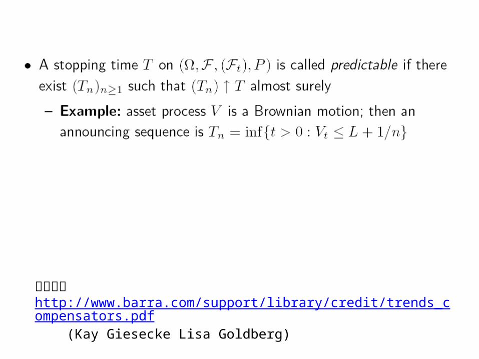
資料來源http://www.barra.com/support/library/credit/trends_compensators.pdf (Kay Giesecke Lisa Goldberg)

Default time

• In the intensity-based approach, the default time will not be a predictable stopping time with respect to the ‘enlarged’ filtration

• The occurrence of the default event comes as a total surprise.

• For any date t, the PV of the default intensity yields the conditional probability of the occurrence of default over an infinitesimally small time interval [t,t+dt].

. ( )G G F

Recovery rules

• If default occurs after time T, the promised claim X is paid in full at time T.

• Otherwise, depending on the adopted model,

• In general,

• In most practical,

• The date T,

is paid at

is paid at the maturity dateT

Z

X

( , , , , )DCT X A X Z

1

2

0 : recovery at maturity (DCT of the first type), ( , , , )

0 : recovery at default (DCT of the second type), ( , , , )

Z DCT X A X

X DCT X A Z

and are intrinsic components.F P

2.1.1 Risk-Neutral Valuation Formula • Suppose the underlying financial market

model is arbitrage-free.

• the price process (no coupons or dividends, follows an F-martingale under P*) discounted by the savings account B.

0

{ t}

d{ } { T}

: exp( )

I

all the CF received by the owner of a defaultable claim

(T) I I

t

t u

t

T

B r du

H

D

X X X

Definition 2.1.1 The dividend process D of a defaultable contingent claim , which settles at time T, equals

------------------------------------------------------------------

The default occurs at some date t, the promised dividend At-At- .

( , , , , )DCT X A X Z

d[T, ] [0. ] [0, ]

(T) I ( ) (1 ) .t u u u ut tD X t H dA Z dH

{ } { t} { }[0. ] [0. ](1 ) I I Iu u u u t tt t

H dA dA A A

{ t} { t}[0, ] I Iu u tt

Z dH Z Z

• The promised payoff X could be considered as a part of the promised dividends process A. However, such a convention would be inconvenient, since in practice the recovery rules concerning the promised dividends A and the promised claim X are generally different.

• r.v: Xd(t,T) -- At any time t<T, the current value of all future CFs associated with a given defaultable claim DCT. (set Xd(T,T)= Xd(T). )

Definition 2.1.2

• The risk-neutral valuation formula is known to give the arbitrage price of attainable contingent claims.

• Structural models typically assume that assets of the firm represent a tradable security. (In practice, the total market value of firm’s shares is usually taken as V)

• The issue of existence of replicating strategies for defaultable claims can be analyzed in a similar way as in standard default-free financial models.

d

d 1* [ , ]

d

The (ex-dividend) price process X ( , ) of the defaultable claim

( , , , , ), which settles at time T, is given as

X ( , ) , t [0.T). (2.2)

where X ( ,

t P u u tt T

T

DCT X A X Z

t T B E B dD F

T T

d) X ( ).T

• Assume is generated by the price processes of tradable asset.

• Otherwise, when the default time τ is the first passage time of V to a lower threshold, which does not represent the price of a tradable asset (so that τ is not a stopping time with respect to the filtration generated by some tradable assets), the issue of attainability of defaultable contingent claims becomes more delicate.

F

,

, 1* [ , ]

We examin in some detail the two special cases of expression

(2.2). price process ( , ) of a defaultable claim equals,

for 1,2 : ( , ) : , (2.3u

d i i

d i it P u tt T

X T DCT

i X t T B E B dD F

1{ } { T} {t T} [0. ]

2{ } {t T} [0. ] [0, ]

)

where

( I I )I ( ) (1 ) ,

and

I I ( ) (1 )

t

t

T u ut

T u u u ut t

D X X t H dA

D X t H dA Z dH

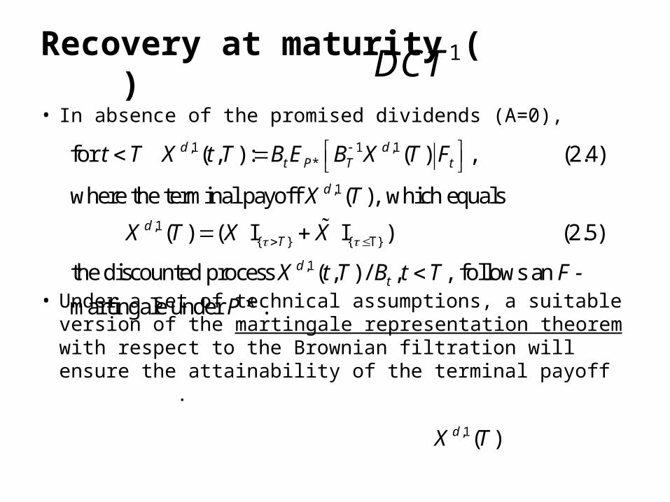
Recovery at maturity ( )

• In absence of the promised dividends (A=0),

• Under a set of technical assumptions, a suitable version of the martingale representation theorem with respect to the Brownian filtration will ensure the attainability of the terminal payoff .

1DCT

,1 1 ,1*

,1

,1{ } { T}

for ( , ) : ( ) , (2.4)

where the terminal payoff ( ), which equals

( ) ( I I ) (2.5)

the discounte

d dt P T t

d

dT

t T X t T B E B X T F

X T

X T X X

,1d process ( , ) / , , follows an

martingale under .

dtX t T B t T F -

P *

,1( )dX T

• In absence of the promised dividends (A=0), (2.3) defines only the pre-default value of a defaultable claim.

• The value process vanishes identically on the random interval [τ,T].

Recovery at default ( )2DCT

,2 ( , )dX t T

,2the discounted process ( , ) / , , will follows an

martingale under only when we consider this process prior

to the default time .

dtX t T B t T

F -

P*,

Another possible solution

• Assuming that the recovery payoff Zτ is invested in default-free zero-coupon bonds of maturity T.

• When we search for the pre-default value of a defaultable claim, such a convention does not affect the valuation problem for DCT2.

,2 ( , ) on [ ,T]dX t T

1

Under this convention, one finishes with a defaultable claim of

the first type with ( , )X Z B T

A formal justification of Definition 2.1.2 based on the no-arbitrage argument.

• Price process of k primary securities Si, i=1,…,k– Si –semimartingales , i=1,…,k-1

and non-dividend-paying assets

– Sk : saving account

• A trading strategy process:

2.1.2 Self-Financing Trading Strategies

,

the discounted price processes / .

kt t

i it t t

S B

S S B

0( ,..., ), -predictablek F-

• Assume that we have an additional security that pays dividends during its lifespan according to a process of finite variation D, with D0 =0. Let S0 denote the yet unspecified price process of this security.

• Since we do not assume a priori that S0 follows a semimartingale, we are not yet in a position to consider general trading strategies involving the defaultable claim anyway.

• Suppose that we purchase one unit of the 0th asset 00(at time 0, initial price ). Then hold it to time T, and invest

all the proceeds from dividends in a savings account.

Consider a - - strategy: (1,0,...,0, ),

wealth process ( ) equals

k

S

buy and hold

U

0

00 0 0

( ) , [0, ] (2.6)

with some initial value ( ) . We assume that the

strategy introduced above is - ;

. ., for every [0, ]

kt t t t

k

U S B t T

U S

self financing

i e t T

0 0

0 0 [0, ] ( ) ( ) . (2.7)k

t t t u utU U S S D dB

Lemma 2.1.11

0 0 10 0 [0, ]

The discounted wealth ( ) ( ) of a self-financing

trading strategy satisfies, for every [0, ] ,

( ) ( ) . (2.8)

Proof. We define an auxiliary

t t t

t t u ut

U B U

t T

U U S S B dD

0

0 [0, ]

ˆ process ( ) by setting

ˆ ( ) : ( ) . In view of (2.7), we have

ˆ ˆ ( ) ( ) ,

ˆand so the process ( ) follows a semimartingale.

kt t t t t

kt t u ut

U

U U S B

U U D dB

U

1

1

1

1 1

1

0

1

ˆ ˆ ( ) ( )

exp( ),

ˆ ( (

)) t t t t

k kt t

t t

t t

t t tt t t

t

t u t t

B dB B dB

B dU U dB

B dD

B

d B U

B d

d

D

r du B r B

1 1 1 1

1 0 1 0 10 0 0 [0, ]

0 0 1

[ , ]

( ) 0

Integrating the last equality

( ) ( ) ,

For every [0, ],

( ) ( ) . (2.9)

t

t t t t t t t t t t

t t t u ut

T t T t u ut T

B dB B dB B r B B r B

B U S B U S B dD

t T

U U S S B dD

2.1.3 Martingale Measures• Goal: derive the risk-neutral valuation formula for the ex-

dividend price

• Assume:

0

the model is arbitrage-free

it admit a (not necessarily unique)

spot martingale measure * equivalent to .

the discoun

tS

P P.

1

ted price

of any non-dividend paying primary security

the discounted wealth process ( )

of any self-financing trading strategy (0, ,..., )

i

t

k

S

U

admissible

follow martingales under *.

In addition, the trading strategy (in Sect 2.1.2) is also admissible,

so that ( ) follows a *-martingale with repect to the filtration . tU

P

P F

Proposition 2.1.1

th

0 0 0

We make an assumption that the market value at time t of the

0 security comes exclusively from the future dividends stream;

0. In view of this convention, we shall refer to as

the -

T TS S S

ex div

th of the 0 asset, e.g., a defaultable claim.idend price

0

0 1* [ , ]

The ex-dividend price process satisfies, for t 0, ,

(2.10)t t u u tt T

S T

S B B dD F

PE

*

Proof.

In view of the martingale property of the discounted wealty

process ( ), for any 0, we have

( ) ( ) 0.

Taking into account (2.9), we thus obtain

t

T t t

U t T

U U F

PE

0 0 1* [ , ]

0 0

.

Since by assumption 0, the last formula yields (2.10).

t T u u tt T

T T

S S B dD F

S S

PE

Proposition 2.1.1

1

0

0

Let us now examine a (0, ,..., ).

The associated wealth process ( ) equals ( ) .

A stratigy is said to be if ( ) ( ) ( )

for every 0,

-

k

k i it t ti

t tsel

general trading strateg

f finan

y

U U S

ng Ui G

t

c U

0

[0, ] [0, ]0

, where the ( ) is defined as

follows:

( ) :

.k

i it u u u ut t

i

gains processT G

G dD dS

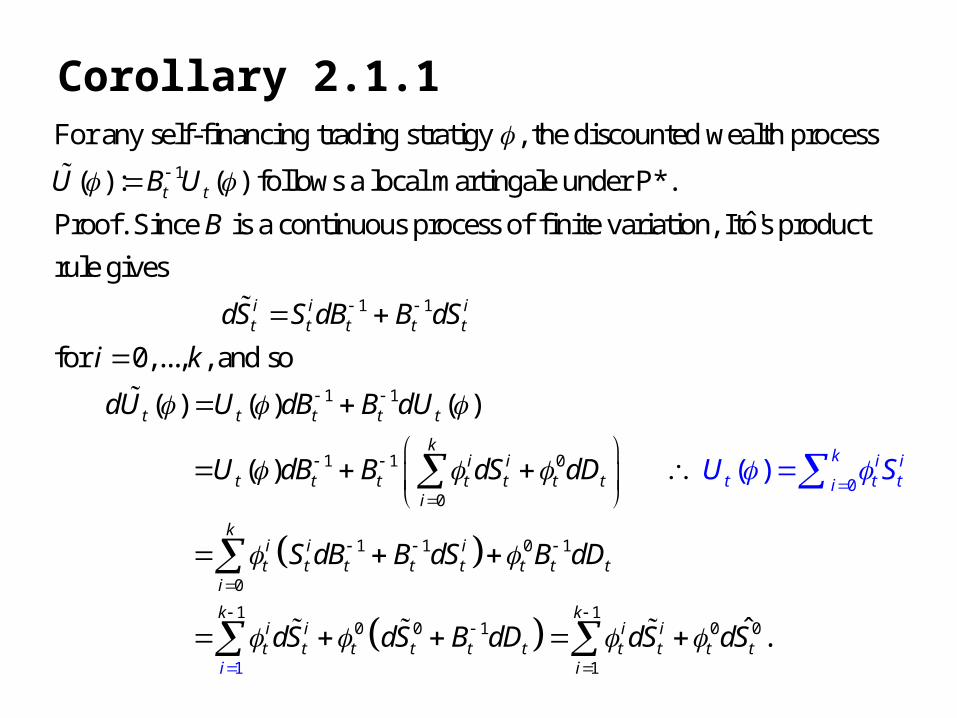
Corollary 2.1.1

1

For any self-financing trading stratigy , the discounted wealth process

( ) : ( ) follows a local martingale under *.

ˆProof. Since is a continuous process of finite variation, Ito's productt tU B U

B

P

1 1

1 1

1 1 0

00

rule gives

for 0,..., , and so

( ) ( ) ( )

( )

(

)

i i it t t t t

t t t t t

ki i

t t t t t

k i it t tt

iit

dS S dB B dS

i k

dU U dB B dU

U dB B dS dD U S

1 1 0 1

0

1 10 0 0

1

1 0

1

ˆ .

ki i it t t

i

t t t t ti

k ki i i it t t t t t t t t t

i

S dB B dS B dD

dS dS B dD dS dS

0

0 0 1

[0, ]

0

ˆwhere the process is given by the formula

ˆ : .

ˆTo conclude,ot suffices to observe that in view of (2.10) the process

satisfies

t t u ut

t

S

S S B dD

S

0 1* [0, ]

ˆ ,

and thus it follows a martingale under *.

t u u tTS B dD F PE

P

Remarks• It is worth noticing that represents the discounted cum-

dividend price at time t of the 0th asset.

• Under the assumption of uniqueness of a spot martingale measure , any -integrable contingent claim is attainable, and the valuation formula can be justified by means of replication. Otherwise - that is, when a martingale probability measure is not unique - the right-hand side of (2.10) may depend on the choice of a particular martingale probability.

• In this case, a process defined by (2.10) for an arbitrarily chosen spot martingale measure can be taken as the no-arbitrage price process of a defaultable claim.

*P *P

0ˆtS

*P