1

2010 年两岸暑期学术交流 专题报告

利用地震訊號测量滑波发生位置以及大小Monitoring Landslide with Seismic Waveforms

作者 清华大学 物理系 黄柏轩

指导老师 中国科学技术大学 地空物理系 倪四道教授

日期：2010.8.25

Abstract Because the seismic signals generated by large landslide (volume

>10 M ), like 2005 Mt. Stellar avalanche in this study, can be detected by seismic stations, we are able to reconstruct the landslide by simulating the seismic signals with single force, and then attain the theoretical value of the energy the landslide released. Compiling seismic data from stations near Mt. stellar, Alaska, we found that the

magnitude of the single force is about the scale of 〖〗 ^

D_Dd__________-ðϨϨ________________ 〖 〗 ^

^_D_Dd__________ˮĻϨϨ_ 〖〗^ ^

Then, we compare the volume of the landslide estimated by seismic signals with that by airborne observation to test our hypothesis of the mechanism of the landslide. We assume big landslide happened on steep slope can be analogous to the motion of free fall body. The result differs from the airborne observation by 4 times, which may partially stems from the imperfection of the free-

2

fall hypothesis. Thus, we tried other landslide mechanisms based on horizontal single force, which are proposed for good compatibility (Mario La Rocca,1993, and Emily E. Brodsky, 2003). Nevertheless, the situation worsened, indicating that there must be other causes of the error. The inaccuracy of parameters of the earth crust model used in signal simulation is another problem. The topography the landslide area and the property of the crust can make considerable influence on the seismic waves. Without necessary geological and geographic data, the precision of the estimation can hardly make breakthrough advance.

Index

Motivation and purpose………..3

Introduction…………………….3

Hypothesis………………….…...6

Methodology and procedures.…6

Discussion……………..………15

Conclusion..................................16

Acknowledgments……………16

References………………16

3

Motivation and purpose Thanks to glacial earthquakes caused by avalanches and landslides, monitoring

low frequency seismic signals enables seismologists to detect landslides and avalanches occur in remote region where people can barely visit, such as arctic region and Antarctic region. Analysis of the frequency, amplitude and the duration of these low-frequency signals provide crucial geophysical information about the landslides, such as locations and scales, which help understand more about the mechanism of avalanches in glacial area. As climate change has become a severe issue, researching avalanches through analyzing earthquake signals started being view as an important resort to help investigate how avalanches occur with given thermal condition. (Huggel, C., Gruber, S. 2008). These studies not only tell us how climate change

4

glacial environment, but help prevent avalanche hazard. Therefore, more intensive further studies of the low-frequency seismic waves are necessary. This paper describes how to simulate low-frequency signals to estimate the size of landslides. The signals we picked here is from landslide of Mt. Stellar, Alaska.

Introduction Earthquakes may be caused by several reasons. Tectonic earthquakes caused by tectonic activities, volcanic earthquakes caused by volcanic activities, collapse earthquakes caused by collapses of caves and mines, and artificial explosion earthquakes of nuclear weapon tests are all often heard and play crucial roles in our lives.

Although being less famous, landslides cause earthquakes as well. A huge landslide of scale of

can induce a small to moderate tremor (

M<5 ). Some of the earthquakes are smaller, only to be detected by regional seismic stations, which are located not farther than 1000km from the epic center. On Sept.14.2005, however, a landslide

of 50 in Alaska (Fig.1) was detected by seismic stations around the globe. It was positioned soon after, and being found located in remote southeast Alaska wilderness, where can only be reached by planes. The quickest way to estimate the size of the landslide is to analysis the seismic signals it generated. This study aims at reconstruct the size of the exceptionally big earthquakes with long period seismic waves through model summation method and the. Besides, I will use the polarization analysis of Rayleigh waves and short-period P waves to locate the position of the landslide. The 2005 Mt. Steller landslide

Figure1. Photo showing the flow path through the glacial valley of the south flank of Mr.Steller and the runout area of the rock-ice avalanche on the Bering Glacier. For scale, refer to Fig.2

5

Mt.Steller (3236ma.s.l.,60 ) is part

of the Waxell Ridge, which separates the Bagley Ice Field from Bering Glacier (Fig. 1). The Waxell Ridge is a very remote area that almost only visited from the air. The 14 September 2005 rock-ice avalanche from Mt. Steller was identified because its associated seismic signals were recorded at seismometers throughout

Alaska and around the world. The Alaska Earthquake Information Center reported that the event had an equivalent local magnitude of 3.8, while analysis of global long period waves yielded a magnitude of 5.2 (G. Ekstrom, personal communication, 2005). Due to the difficult access conditions of Mt. Steller, the reconstruction of the ice-rock avalanche was based on remotely operating systems such as satellite imagery, airborne observations, and seismic recordings.

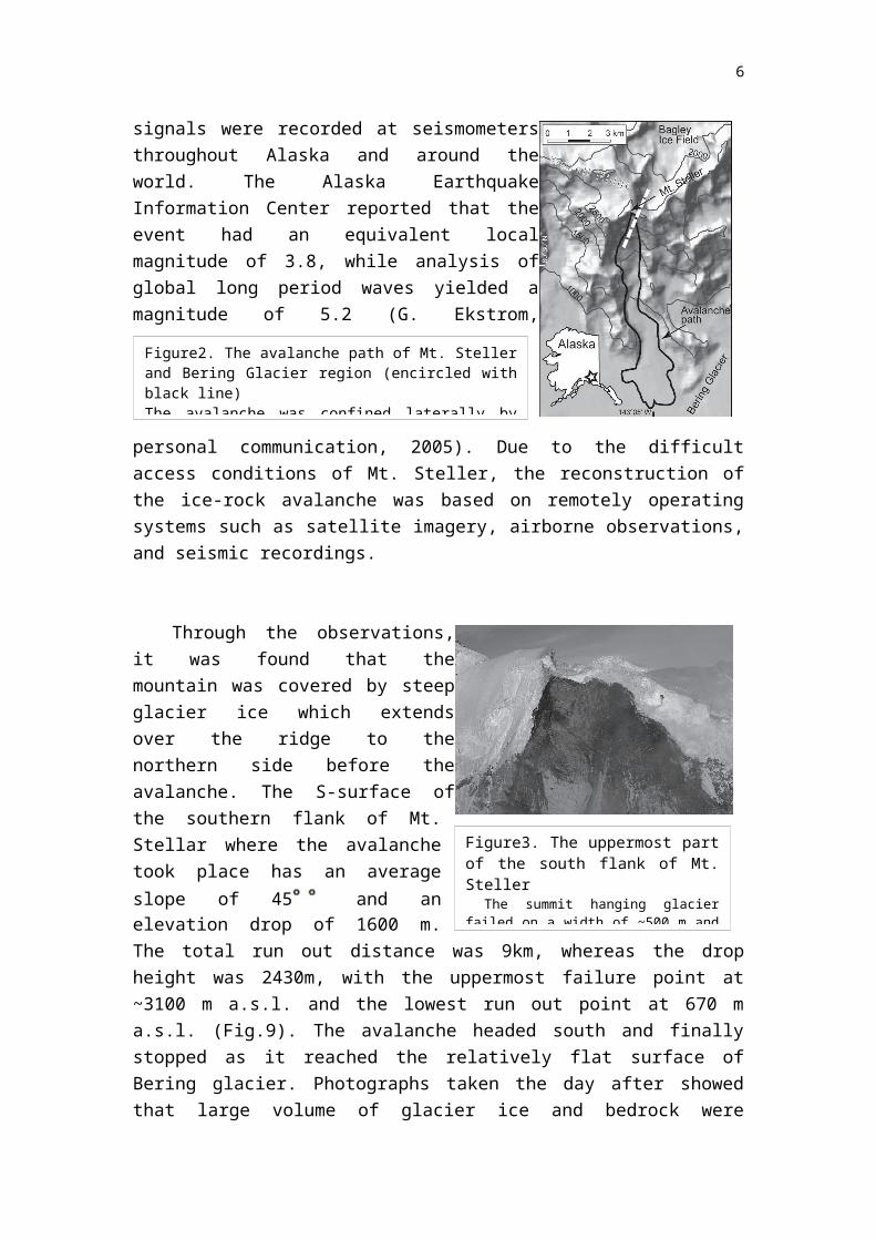
Through the observations, it was found that the mountain was covered by steep glacier ice which extends over the ridge to the northern side before the avalanche. The S-surface of the southern flank of Mt. Stellar where the avalanche took place has an average slope of 45 and an elevation drop of 1600 m. The total run out distance was 9km, whereas the drop height was 2430m, with the uppermost failure point at ~3100 m a.s.l. and the lowest run out point at 670 m a.s.l. (Fig.9). The avalanche headed south and finally stopped as it reached the relatively flat surface of Bering glacier. Photographs taken the day after showed that large volume of glacier ice and bedrock were involved in the landslide. It is estimated from

observation of the photographs that 3 to 4.5 million of glacier ice with ice thickness of 20 to 30m m failed. Due to the lack of precise topographic data, the failure volume of rock is difficult to evaluate. A crude estimation suggested that about

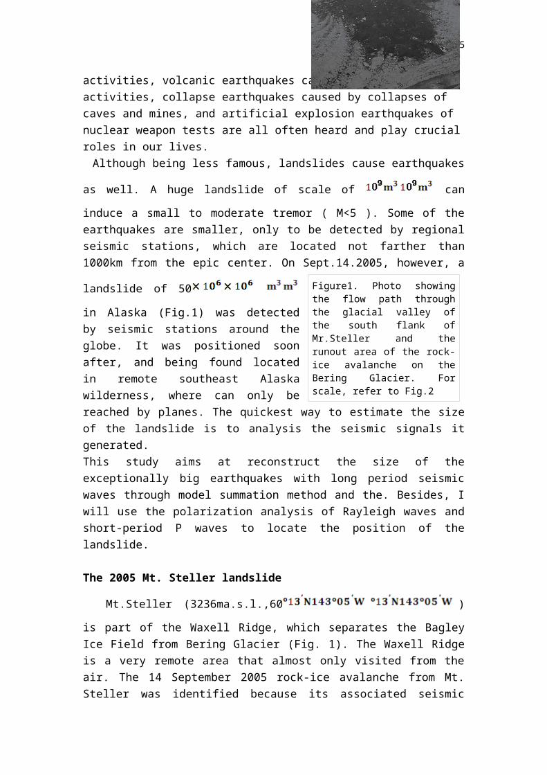
Figure2. The avalanche path of Mt. Steller and Bering Glacier region (encircled with black line)The avalanche was confined laterally by the valley, and spread out at the relatively flat surface of Bering Glacier.

Figure3. The uppermost part of the south flank of Mt. Steller The summit hanging glacier failed on a width of ~500 m and an elevation range of ~200 m. The ice thickness is in the range of 20–30 m.

6

10 to 20 million of bedrock failed. The total avalanche volume deposited on Bering Glacier can be reconstructed with an area of 4 and an average deposit thickness of 10 to 15 m using the undulating topography of the moraine ridges that were filled by the avalanche deposits as a height reference. This yields a total

avalanche volume of 40 to 60 million .

Force model of the landslideThe occurrences of nature earthquake are because of the tectonic motion. Under

the governance of Newton’s 3rd law of motion, the force of the tectonic motion must be generated in pairs with opposite direction and equal magnitude. We call the dual forces “coupling force.” To satisfy conservation of angular momentum in the coordinate of the Earth, the torques acting on faults must be a pair, too. Torques causing the earthquake can be sorted into two types – alone the fault and perpendicular to the fault.

On the other hand, earthquakes yield by landslides and avalanches are not necessarily rendering coupling force, for the reacting force acting on the sliding mass of rocks or ice, which is discrete from the bedrock and have a loose structure, will not propagate through ground. Hence, only the force acting on the bedrock will be recorded by seismograms. This force, which cause earthquake of landslide, is called “single force.”

Single force is actually a force drop due to the recoil of the ground when a large mass starts sliding down. Since rock inherits certain elasticity, the ground is actually elastic in microscope. Before the landslide, the bedrock yields to a reacting force caused by the gravitational force acting on the mass, and thus slightly transformed. When the landslide starts, the pressure vanished, and the bedrock recoils like a spring. (Refer to Fig.4).

This single force model has been adopted by several authors (Mario La Rocca et al., 2004) and proved applicable.

Frictional force

Figure 4.The mass is in equilibrium prior to the landslide, and the bed rock yields a reacting force caused by the gravitational force and the frictional force, slightly transformed. After the landslide, reacting force vanished, and the bedrock recoils like the spring.

gravitational force

Recoil

7

Theory for landslide detecting Generally speaking, landslides with scale of cubic kilometer are detectable around

the world. On the other hand, signal of smaller landslides can only be found in regional stations.

According to empirical formula garnered by observation, time durations of most

earthquakes are proportional to , where M is the magnitude of the earthquake.

That is, durations of earthquakes below Ritcher magnitude 7 are usually shorter than 20 seconds. The typical duration for a magnitude 5 earthquake is 2 seconds.

Inheriting tremendous energy, tectonic earthquakes must radiate seismic waves with high frequencies (~1 Hz) to give out stored strength in few seconds. Nevertheless, since landslides inherit much less energy and have much longer durations, they generate relatively long period seismic waves which are outside the pass band usually used to monitor tectonic earthquakes. Appling pass band of lower frequency (0.05~0.1 Hz), many undiscovered earthquakes when adopting high frequency filter are revealed, and some of which are outside tectonically active zones. By analysis seismic waves and through simulation and other remotely operating systems, such as satellite imagery, we can distinguish earthquakes caused by landslides with others. This discovery opens a door for seismologist to learn more about big avalanches and landslides.

Hypothesis Since the southern flank of Mt. stellar, where the avalanche took place was steep.

We assume that the single force of the landslide can be considered as a vertical force. With the snow as lubricant, the coefficient of fiction of the bedrock is small. We consequently speculate that the process of the landslide may be similar to that of free fall motion, so the final velocity of the landslide is known with the formula:

Then we can calculate the magnitude of single force with following equation:

mass

8

Then, we get the volume of the landslide if we know the density

()/√D_Dd__________

With some rearrangement:

Another postulate is that the mass must be rigid instead of deformable; there is no inner dissipation of energy within the sliding mass.

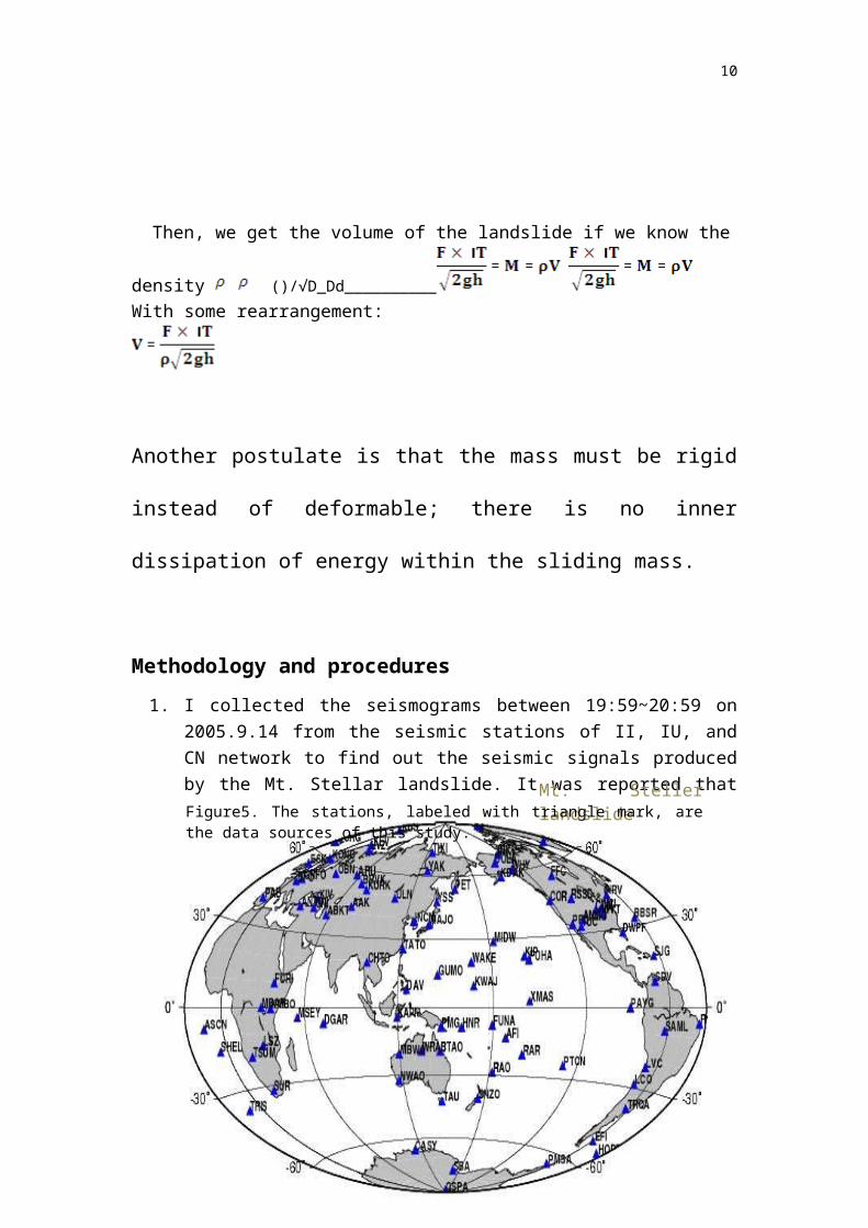
Methodology and procedures1. I collected the seismograms between 19:59~20:59 on 2005.9.14 from the

seismic stations of II, IU, and CN network to find out the seismic signals produced by the Mt. Stellar landslide. It was reported that the landslide generated global long period waves which yielded a magnitude of 5.2 (G.

Ekstrom, personal communication, 2005)

Mt. Steller landslideFigure5. The stations, labeled with triangle mark, are the data sources of this study.

9

2. The waveforms we see on the seismogram so far are not what the landslide actually generated. The error caused by the instruments must be considered. To attain the actual seismic waveforms, the removal of frequency responses of the seismometers is necessary.

3. Some of the seismograms from some stations are useless and discarded, for they didn’t record significant signals during the landslide.

4. Next, we have to remove the noise from the useful part of the seismic signals

so that we can identify more detailed event during the landslide. Since the signals of landslides have longer wave periods than tectonic earthquakes, I choose a pass band of 0.05~0.1 Hz to filter the signals (M. Rocca et. al., 2004). Then, I pick out the seismograms with meaningful signals.

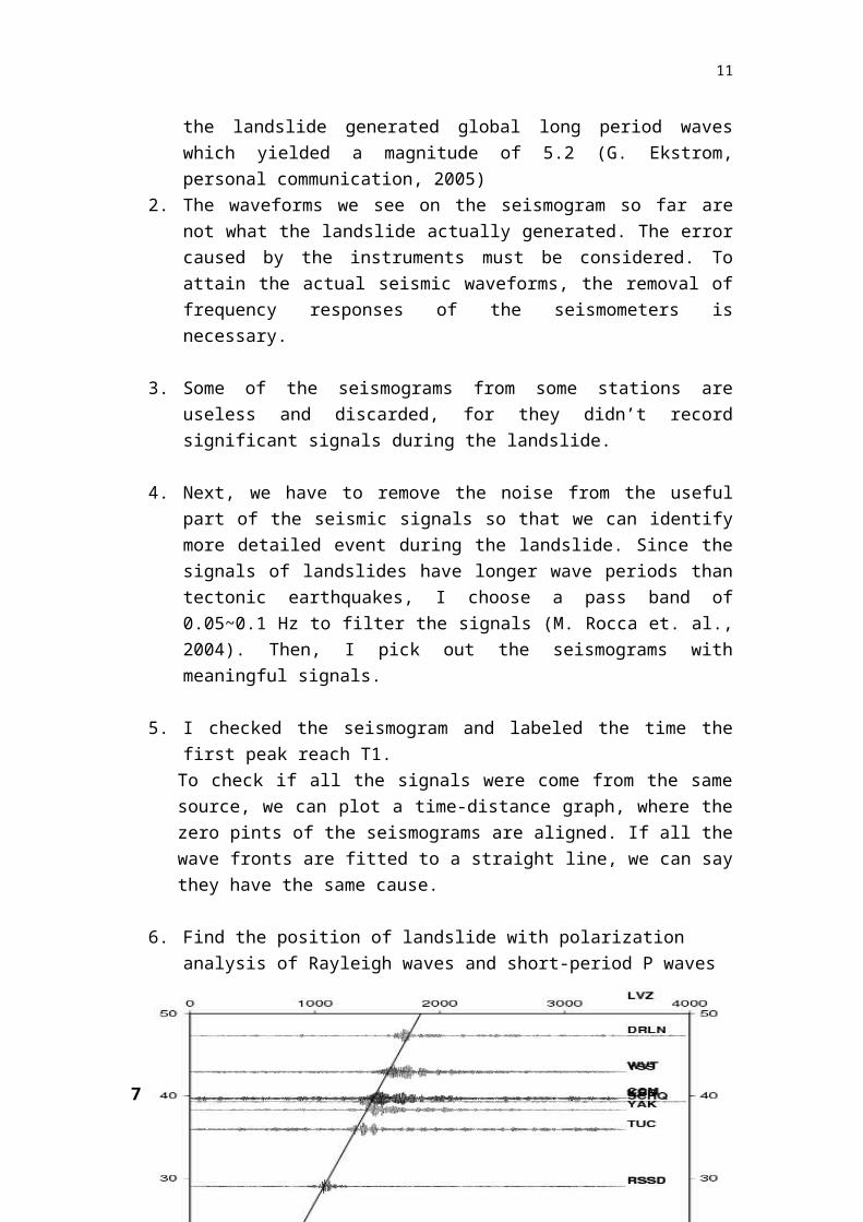
5. I checked the seismogram and labeled the time the first peak reach T1.

To check if all the signals were come from the same source, we can plot a time-distance graph, where the zero pints of the seismograms are aligned. If all the wave fronts are fitted to a straight line, we can say they have the same cause.

6. Find the position of landslide with polarization analysis of Rayleigh waves and short-period P waves

7.

Figure6. The unit of x-axis is second, and the y-axis unit is 100km. The slope of the straight line is the reciprocal of the velocity of the landslide signal, which is constant. The signal detected by the stations lies on the straight line means they are generated by the same source.

10

Use Model summation method to simulate the real waveforms.I simulate the waveforms with three kinds of force source. The forces are in

N (north-south), E (east-west), and Z (vertical) directions. To produce the synthetic waves, I construct an earth model which consists of the density, thickness, and velocity of P wave and S wave of each layer of the curst. Then, I chose the nearest four stations, labeled with COLA, WHY, KDAK, INK (fig. 5) to make comparison with the synthetic wave produced by the model. The four stations are seated less than 1000 km from the force source.

It brings much convenience to focus our study on signals near the epic center. First, the signals are less disturbed by the noise caused by ground property and other seismic events. Second, the frequency dispersions are indistinctive, so the tolerable ranges of the parameters of the earth model are wider, which make our work to estimate the scale of the landslide a lot easier.

A perfect simulation means that the synthetic wave is completely identical to the real waveform. The more similar the synthetic wave is to the real one, the better simulation it is. In seismological jargon, the perfect simulation has a cross correlation of 1. When the cross correlation is closer to 1, a better simulation are made. In reality, rather than pursuing perfect simulation, the comparisons of some characteristics of the waveforms are a more sensible approach to conduct. Generally speaking, good compactness of amplitudes, frequencies, and arriving times of the signals are fairly enough to pin down an acceptable simulation. In this study, we aimed at finding out the volume and released energy of the landslide, so the fitness of the amplitudes dominates the others.

When the single force is dyne, vertical to the ground, we attain good

simulations, in which the amplitudes of the synthetic and real waveforms are in the same scale.

11

Figure 7-a. the simulation diagrams in Z direction using vertical force

The following four diagrams are the results of four stations lies in distance-to-source order.

The red line is the synthetic waveform detected in Z direction; the black line is the real one.

They are in the same scale when the force is dyne. Amplitude (cm)

Arriving time (100 sec)

Amplitude (cm)

12

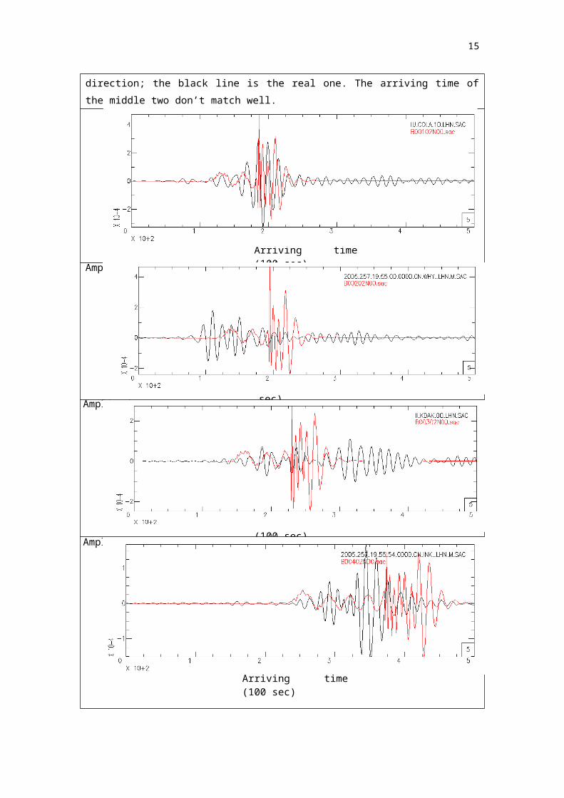
Figure 7-b. the simulation diagrams in N direction using vertical force

The red line is the synthetic waveform detected in N direction; the black line is the real one.

The arriving time of the middle two don’t match well.

Amplitude (cm)

Arriving time (100 sec)

Amplitude (cm)

Arriving time (100 sec)

Arriving time (100 sec)

Amplitude (cm)

13

Arriving time (100 sec)

Amplitude (cm)

Amplitude (cm)

Arriving time (100 sec)

14

Figure 7-c. the simulation diagrams in E direction using vertical force

The red line is the synthetic waveform detected in E (east-west) direction; the black line is the

real one. Base on the mechanism used in model summation method, The vertical single force

doesn’t generate vibrations in east-west direction, so the seismograms of the rest stations are not

shown.

Amplitude (cm)

Arriving time (100 sec)

Arriving time (100 sec)

Amplitude (cm)

15

However, some essays indicate that the effective single force should be in horizontal direction (E. Brodsky et al., 2003). Therefore I also did the simulation using horizontal single force. They fit well, too.

Figure 8-a. the simulation diagrams in Z direction using horizontal force

The red line is the synthetic waveform detected in vertical direction; the black line is the real

one. The amplitude of the two waves are in the same scale. The single force is dyne.

479km

Arriving time (100 sec)

Amplitude (cm)

Amplitude (cm)

Arriving time (100 sec)

16

D

D

Arriving time (100 sec)

Amplitude (cm)

Amplitude (cm)

Arriving time (100 sec)

17

)

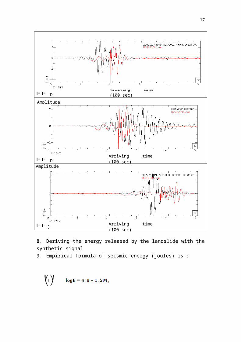
8. Deriving the energy released by the landslide with the synthetic signal9. Empirical formula of seismic energy (joules) is :

, where is the magnitude of the surface wave. According to the postulation, the landslide was caused by sallow vertical single force, which only produces P waves (body wave). We substitute with body-wave magnitude

.

Measured values from the seismograms (refer to Fig.6, Fig.7) :

Arriving time (100 sec)

18

Amplitude of the P wave (A) = 0.02 m Duration (T) ~ 65 seconds The duration of the landslide is shorter than the duration of the signal

because it takes some time attenuate after the landslide. We chose the data from the nearest station, for it shows the shortest duration. As landslides much leave signals on the seismogram, it is impossible the duration of Mt. Stellar landslide to be longer than the shortest duration recorded by the station. Besides, considering attenuation, the actual landslide duration must be shorter.

It was proposed that the maximum durations are based on the rapid amplitude increase and decrease (Caplan-Auerback, J. et al., 2004). We assume the landslide started and ended when the amplitude of the signal is 30% of the maximum amplitude.

Observing seismogram from the nearest station COLA below, sit in the middle of Alaska (Refer to fig.5, 65 __D_Dd__________ዝ ԷϨϨ________________

D_Dd__________ÿԷϨϨ________________ ()/_D_Dd__________-ĝϨϨ________________

()/()___⇨_⇪_ _ _ _ _ _ _⇬ ⇰ ⑄ ⑆ ⑈⇸ ⒐_⒒_⒔_⒘_⒜_⒞_⒢_ⓨ_⓪_ _ _⓬ ⓰

Amplitude (cm)

Figure9. The duration of the landslide can be view as the moment the amplitudes change rapidly. T0 is the starting time, and T1 is the ending time. The blue lines mark 30% of the maximum amplitude.

Arriving time (100 sec)

T1T0

19

Distance in degree ()/ R is the radius of the Earth.

= .

Substitute into (2), and calculation shows that the energy released by the Mt. Stellar avalanche is 2.8 joule, which is equivalent to the explosion of 67 kg of TNT.

10. calculation of the volume of the landslideI.Supposing the landslide was a rigid body, and the process of the slide was

similar to a free fall motion. Then, we can calculate the single force by the formula beneath:

Where ()/√________________________________________________________________________

___________________________________________________________________________

___

Making some change of the formula, we can estimate the falling volume of the landslide:

Where ^_D_Dd__________ŨĬϨϨ________________ 〖 〗 ^

D_Dd__________ ̛ĻϨϨ_ . The drop height is about 2430m, and the duration of the landslide is about 20 seconds. Use the result of the simulation, the scale of the

single force is ()/(√)(〖〗^)/(√())_D_Dd__________ᚎʲϨϨ________________

___ million cubic meters.

20

The volume of the landslide of Mt. Stellar, Alaska is about ()/(√( /))()/(√)_D_Dd__________ᴼԷϨϨ________________

〖 〗 ^_D_Dd__________ƤĬϨϨ________________ _

_D_Dd__________ ᩬԷϨϨ________________

D_Dd__________ÒĝϨϨ________________

D_Dd__________ĻĝϨϨ________________ __ㇴ_ㇶ_ㇸ_ㇼ_㑄_㑆_㑊_㒤_㒦_㒨_㒬_

㡄_㡆_㡈_㢐_㢒_㢖_㢞_㣤_㣦_㣨_㣬_㤴_膒槽鷖勢藖勈劯旖体腄______________

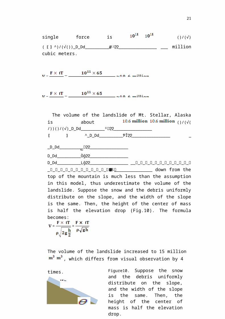
__ down from the top of the mountain is much less than the assumption in this model, thus underestimate the volume of the landslide. Suppose the snow and the debris uniformly distribute on the slope, and the width of the slope is the same. Then, the height of the center of mass is half the elevation drop (Fig.10). The formula becomes:

The volume of the landslide increased to 15 million , which differs from visual observation by 4 times.

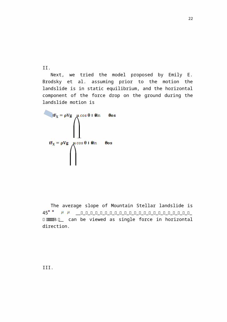
II.Next, we tried the model proposed by Emily E. Brodsky et al. assuming prior

to the motion the landslide is in static equilibrium, and the horizontal component of the force drop on the ground during the landslide motion is

Figure10. Suppose the snow and the debris uniformly distribute on the slope, and the width of the slope is the same. Then, the height of the center of mass is half the elevation drop.

21

The average slope of Mountain Stellar landslide is 45 __ㇴ_ㇶ_ㇸ_ㇼ_

㑄_㑆_㑊_㒤_㒦_㒨_㒬_㡄_㡆_㡈_㢐_㢒_㢖_㢞_㣤_㣦_㣨_㣬_㤴_膒槽鷖勢藖勈劯旖体腄__ can be viewed as single force in horizontal direction.

III.

Lastly, we used the force model

D_Dd__________ƤĝϨϨ______the landslide volume, where/(^ )D_Dd__________ѴȺϨϨ________________

^_D_Dd__________ŨĬϨϨ________________

^__________________________________________________________________________

___

Since the the avalanche was about 99,000 ~1.5 M .

Discussion Summing up the above results, the scale of the landslide volume is 4~6 times

smaller than the airborne observation. There are several possible causes. I. Incorrect simulationThe simulation may be incorrect, which means the single force is not

〖 〗 ^ D_Dd__________مĻϨϨ________________()

()/(√)D_Dd__________ჟԷϨϨ_____ ()

()/(√)D_Dd__________ჟԷϨϨ________________ D_Dd__________ĝ� ϨϨ________________

22

〖〗^〖〗^ _______________________________________㶞_㶠_㶤_䁄_

II. Crude model The theoretic models explaining the mechanism of the landslides so far are too simple to derive accurate results. Like Emily E. Brodsky et al. written in their paper in discussion of the force model:

The mobility method has been often criticized as inapplicable to deformable slides with internal dissipation and subject to geometric biases.

To certain degree, avalanche and landslide can be viewed as a sort of fluid, rather than rigid body. Bring hydromechanics into the physics of landslide and avalanche will resolve the problem of internal dissipation.

III. Geological data of the plate of Alaska regionAs for the result of simulation, readers can easily find that the closer the seismic

station is to the source, the better the simulation is. Since we assume ground is homogeneous in the earth model, the distance of the station to the epic center is the only variable between stations. Observing the compactness of the four stations in each direction in fig. 6, the arriving time of the phase of synthetic wave gradually shift away from the real wave. The error stems from the inaccuracy of the earth model used in simulation, which can be improved by adjusting the parameters of the densities, elasticity and wave velocities of earth crust model. To get this geological data, more geological investigations of the crust of Alaska and other Antarctic region are necessary.

IV. Band Pass Range The signal pass through the band pass filter is incomplete. Some signals caused by

the failing rock are filtered out. To find the best band pass range not only requires knowledge but also experiences, since we don’t understand the actual mechanism work behind landslides.

The pass band I picked is 0.05Hz~0.1Hz, which was used and proved successful (M. Rocca et al., 2004). However, the landslide M. Rocca studied is triggered by volcano eruption, whose mechanism may be different from glacial landslide. On the other hand, it was suggested to use 0.006 Hz~0.02 Hz as pass band for glacial earthquakes (Göran Ekström, 2003). Nonetheless, whether it will bring a better-defined signal is uncertain, for there are still too much undetermined variables so far.

23

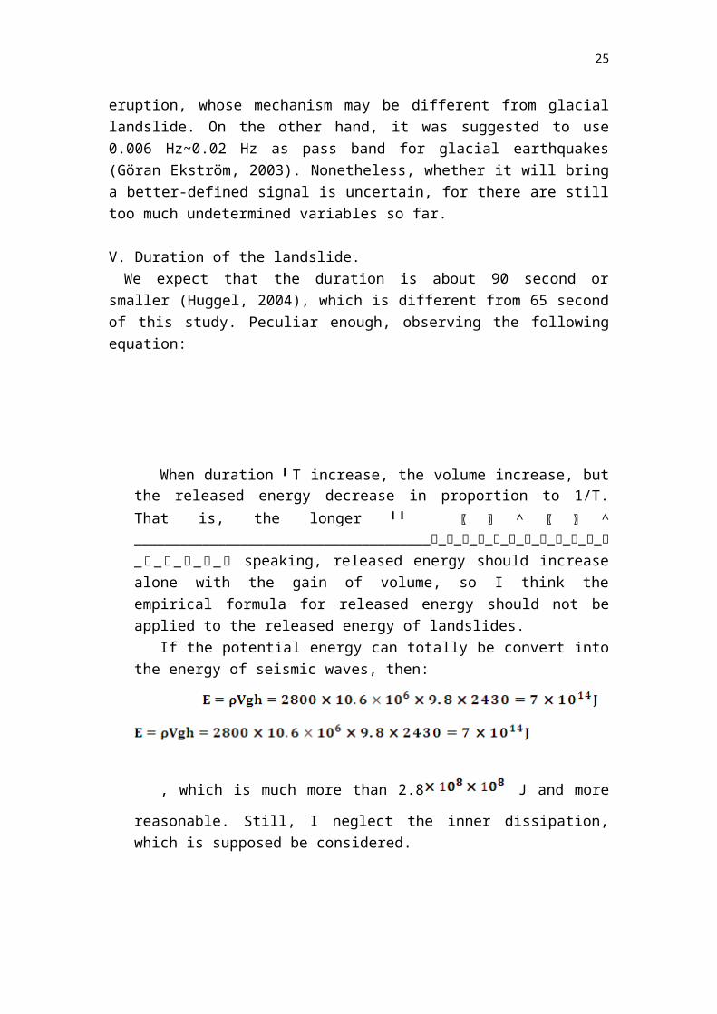
V. Duration of the landslide. We expect that the duration is about 90 second or smaller (Huggel, 2004), which is different from 65 second of this study. Peculiar enough, observing the following equation:

When duration T increase, the volume increase, but the released energy decrease in proportion to 1/T. That is, the longer 〖 〗 ^ 〖 〗 ^

_______________________________________㶞_㶠_㶤_䁄_䁆_䁈_䁌_䂘_䂚_䂜_䂠_䃬_

䃮_䃰_䃲_䃴_䃶 speaking, released energy should increase alone with the gain of volume, so I think the empirical formula for released energy should not be applied to the released energy of landslides.

If the potential energy can totally be convert into the energy of seismic waves, then:

, which is much more than 2.8 J and more reasonable. Still, I neglect

the inner dissipation, which is supposed be considered.

ConclusionAmong the three methods of estimating the volume of Mt. Steller landslide,

the free-fall model is the best one, which gives a result of 1.5 million cubic meters. The answer differs from the visual observation by 4 times, for several possible sources of error discussed above, including incorrect simulation, crude model, lack of geological data, and improper choose of the pass band. Even so, the model brings us an answer that is in correct scale of magnitude.

Neglecting the inner dissipation and the dissipation of friction, the released

energy of the avalanche of Mt. Steller is about DDd䬀⻠Ɨ½The hypothesis used in this study may not be totally right, but it practically

give an answer that is helpful for us to get better understanding of the landslide.

The landslide of Mt. Steller is one of the biggest landslides that have ever happened on Earth. The seismic signal it produced was so clear that it gives us a chance to understand more about avalanches by seismology means. To understand why the landslide happened is the most important topic because

24

there are innumerable mountains in Alaska and arctic region that are in the same condition as Mt. Steller were before its sudden unexpected collapse. If we can find out the cause, we will save considerable amount of people in the future. If we can estimate volume of a landslide beforehand, we may be able to estimate the number of injuries and the degree of damage of the landslide-stricken region before the medical aid and disaster relief could reach some remote regions.

More studies of similar landslides are needed to improve the model and the theory we used.

Acknowledgments

指导教授 倪四道

指导师兄 曾祥方 崇加军

谢均 吳澄波

陈伟文包峰

References Göran Ekström, et al., Glacial Earthquakes, Science 302, 622 ,2003.

Bruce A. Bolt, Earthquakes 4th edition, June 23, 1999

Christian Huggel et al., The 2005 Mt. Stellar, Alaska, Rock-Ice Avalanche: A Large Slope Failure in

Cold Permafrost, 2008.

Mario La Rocca, Dannilo Gualluzzo et. al., Seismic Signals Associated with Landslides and with a

Tsunami at Stromboli Volcano, Italy, 2004.

Emily E. Brodsky et al., Landslide basal friction as measured by seismic waves, Geophysical

research letters, vol. 30, No, 24, 2003. Caplan-Auerbach, J., Prejean, S.G. & Power, J.A. 2004. Seismic recordings of ice and debris

avalanches on Iliamna Volcano (Alaska). Acta Vulcanologica 16: 9-20.

Mario La Rocca, Dannilo Gualluzzo et. al., Seismic Signals Associated with Landslides and

with a Tsunami at Stromboli Volcano, Italy. , Bulletin of the Seismological Society of America, Vol.

94, No 5, pp. 1850~1867, October 2004.

C. Huggel, J. Caplan-Auerbach, and R. Wessels, Recent Extreme Avalanches: Triggered by Climate

Change? Eos, Vol. 89, No. 47, PAGES 469–470, 18 November 2008.

25