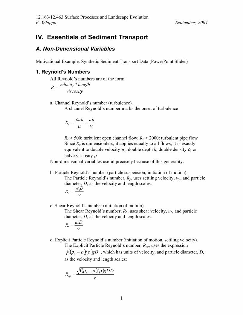
12.163/12.463 Surface Processes and Landscape Evolution K. Whipple September, 2004

IV. Essentials of Sediment Transport

A. Non-Dimensional Variables

Motivational Example: Synthetic Sediment Transport Data (PowerPoint Slides)

1. Reynold’s Numbers All Reynold’s numbers are of the form:

viscosity

lengthvelocityR

*=

a. Channel Reynold’s number (turbulence).A channel Reynold’s number marks the onset of turbulence

!µ

" huhuRe

==

Re > 500: turbulent open channel flow; Re > 2000: turbulent pipe flow Since Re is dimensionless, it applies equally to all flows; it is exactly equivalent to double velocity u , double depth h, double density ρ, or halve viscosity µ.

Non-dimensional variables useful precisely because of this generality.

b. Particle Reynold’s number (particle suspension, initiation of motion). The Particle Reynold’s number, Rp, uses settling velocity, ws, and particle diameter, D, as the velocity and length scales: Rp =

wsD

!

c. Shear Reynold’s number (initiation of motion). The Shear Reynold’s number, R*, uses shear velocity, u*, and particle diameter, D, as the velocity and length scales:

!

DuR

*

*=

d. Explicit Particle Reynold’s number (initiation of motion, settling velocity). The Explicit Particle Reynold’s number, ( )( )gDs !!! "

Rep, uses the expression , which has units of velocity, and particle diameter, D,

as the velocity and length scales:

( )( )

!

""" DgDR

s

ep

#=

1

12.163/12.463 Surface Processes and Landscape Evolution K. Whipple September, 2004

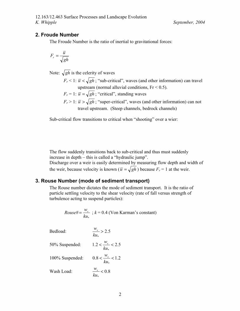
2. Froude Number The Froude Number is the ratio of inertial to gravitational forces:

gh

uFr =

Note: gh is the celerity of waves

Fr < 1: ghu <

Fr = 1: ghu =

Fr > 1: ghu >

; “sub-critical”, waves (and other information) can travel upstream (normal alluvial conditions, Fr < 0.5).

; “critical”, standing waves

; “super-critical”, waves (and other information) can not travel upstream. (Steep channels, bedrock channels)

Sub-critical flow transitions to critical when “shooting” over a wier:

The flow suddenly transitions back to sub-critical and thus must suddenly increase in depth – this is called a “hydraulic jump”. Discharge over a weir is easily determined by measuring flow depth and width of the weir, because velocity is known ( ) because Fr = 1 at the weir. ghu =

3. Rouse Number (mode of sediment transport) The Rouse number dictates the mode of sediment transport. It is the ratio of particle settling velocity to the shear velocity (rate of fall versus strength of turbulence acting to suspend particles):

*

#ku

wRouse

s= ; k = 0.4 (Von Karman’s constant)

Bedload: 5.2

*

>ku

ws

50% Suspended: 5.22.1

*

<<ku

ws

100% Suspended: 2.18.0

*

<<ku

ws

Wash Load: 8.0

*

<ku

ws

2

12.163/12.463 Surface Processes and Landscape Evolution K. Whipple September, 2004

4. Non-Dimensional Settling Velocity Several different non-dimensional groupings are used in describing the controls on settling velocity. The standard non-dimensional settling velocity uses the group ( )( )gDs !!! " to accomplish the non-dimensionalization:

( )( )gD

ww

s

ss

!!! "=

*

Dietrich et al (1983) is a key paper tabulating particle settling velocity dependencies on grain size and shape and uses a related variable W* as their non-dimensional settling velocity:

W*= ws*

2

Rp =ws

3

!s " !( ) !( )g#

However, there is a complication since both W* and the drag coefficient CD depend on particle Reynold’s number, Rp. Therefore, some workers use the Explicit Particle Reynold’s number, which is related to the non-dimensional settling velocity, ws*, by the relation:

Rp =wsD

!= ws*Rep

Excel spreadsheet for calculating settling velocity using equations in Dietrich et al (1983) is available on the class website.

5. Shield’s Stress (sediment transport, initiation of motion). Initiation of motion and sediment transport must depend on, at least: boundary shear stress, sediment and fluid density (buoyancy), and grain-size. Early 1900’s Shields (German) did many experiments on sediment transport and determined a non-dimensional grouping that combines these factors and served to collapse a great range of experimental data to a single curve:

( )gDs

b

!!

""

#=

*

Where boundary shear stress can be approximated by the relation for steady-uniform flow, Shields Stress, τ*, can be written as:

( )( )DhS

s!!!

"#

=*

3

12.163/12.463 Surface Processes and Landscape Evolution K. Whipple September, 2004

At the critical condition for initiation of motion, shear stress = τcr, the critical Shields stress is of course:

!*cr =

!cr

"s # "( )gD

Shields plotted against the Shear Reynold’s number, R*, in his original work. This nicely collapses the data, but is difficult to work with in practice, because both τ* and R* depend on u*, meaning iteration is required to find τcr from the plot (recall !"

bu =*

). Therefore, Shield’s diagram is usually recast in terms of the Explicit Particle Reynold’s number by plotting against:

( )( )2

3

2

**

!

"""#

gDRD sep

$===

6. Non-Dimensional Sediment Transport Rate Qs = total volumetric sediment transport rate through a given river cross section. Sediment flux per unit channel width is by definition:

w

Qq ss =

Einstein (the son) worked on the sediment transport problem and first defined the non-dimensional volumetic sediment flux as:

qs* =qs

!s " !( ) !( )gDD=

qs

Rep#

We will write all sediment transport relationships in terms of this (or very similar) non-dimensional group.

7. Transport Stage Transport stage describes the intensity of sediment transport and is defined simply as the ratio of boundary shear stress to the critical boundary shear stress:

crcr

b

sT

*

*

!

!

!

!==

4

12.163/12.463 Surface Processes and Landscape Evolution K. Whipple September, 2004

B. Sediment Transport Relations

1. Bedload Transport: rolling, sliding, saltating Generally:

( )( )!!!" /,,** #= seps Rfq

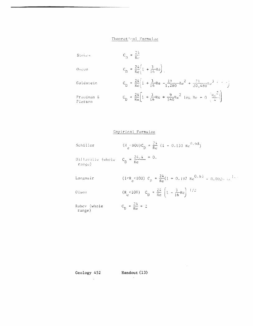
Theoretical relations have been developed, and volumetric flux solved by integrating individual grain motions – much is known about bedload sediment transport. In this class we will restrict ourselves to empirical relations determined in the lab and in the field. They must be applied only to conditions similar to those under which they were determined.

a. Meyer-Peter Mueller (1948) (generalized)

( ) 23

***8

crsq !! "=

Where for gravels, τcr* is a constant: Shields (gravel) ~ 0.06; Parker ~ 0.03 (mixed size gravel); Meyer-Peter Mueller = 0.047 (well sorted fine gravel, at moderate transport stage, Ts ~ 8).

b. Fernandez-Luque and van Beck (1976)

( ) 23

***7.5

crsq !! "=

conditions similar to M-P-M, only at low transport stage (Ts ~ 2).

c. Wilson (1966)

( ) 23

***12

crsq !! "=

conditions similar to M-P-M, only at high transport stage (Ts ~ 100).

Summary:Wiberg and Smith (1989) point out that the observed variation in the transportcoefficient is well captured by a simple dependence on shield’s stress (t*), givinga generalized bedload transport relation:

( )ncrss

q***

!!" #=

23=n

( ) 166.0

**64.98.9ln6.1 !!" =+=

s(R2 for power-law fit: .989)

5

12.163/12.463 Surface Processes and Landscape Evolution K. Whipple September, 2004

d. Bagnold (1977, 1980)

Many versions of the Bagnold relation (empirical fit to lab and field data) exist. A recent adaptation by Bridge and Dominic (1984) is:

qs* = at ! * " !cr*( ) !*

1 2

"! cr*

1 2( )

Where at is a dimensionless constant. Note that Bagnold’s relation is also often written in terms of “unit stream power” (stream power dissipated per unit bed area) ! w =" = #gQS w = $ bu .

e. Parker (1982) Sub-surface Transport Model

Parker (1990, 1992) later revised this empirical relation based on sub-surface D50 (field data) to a surfaced-based model. The difference is whether you need data on the surface D50 or sub-surface D50. For convenience, Parker defined a new, slightly different non-dimensional volume flux of sediment transport to replace the classic qs*:

He also writes the non-dimensional shear stress in terms of the D50 of the subpavement (D50sp) and as a ratio of shear stress to the critical shear stress:

!50

=hS

"s # "( ) "( )D50sp

$

%

& &

'

(

) ) 0.0876 =

**sp

0.0876

Where 0.0876 is the critical shields stress for D50sp, such that φ50cr = 1. Given that D50p/D50sp ~ 2.5, this result implies τ*pcr = 0.035 (ie. lower than the “standard” shields curve result of τ*pcr = 0.06 for uniform-sized gravel).

With these definitions, Parker (1982) fit the following relations to the field data:

( ) ( )[ ]25050*

50

128.912.14exp0025.0

65.195.0

!!!=

""

##

#

w

!50

> 1.65

w*

= 11.2 1 "0.822

!50

#

$

% %

&

'

( (

4.5

6

12.163/12.463 Surface Processes and Landscape Evolution K. Whipple September, 2004

2. Suspended Sediment Transport Suspended sediment transport depends on the product of sediment concentration profiles (for each size class) and the velocity profile, which are of course closely related. Dietrich (1982) presents a graphical tabulation of all sediment settling velocity data as a function of grain size and shape in terms of the non-dimensional

reynold’s number ( ) defined earlier. These

settling velocity W* and non-dimensional grain-size D* or the explicit particle ( )( )

2

3

2

**

!

"""#

gDRD sep

$===

data are critical to computation of sediment concentration profiles. For m size classes, a general expression for suspended sediment flux can be written:

qs = Ciz( )

0

h

!i=1

m

" u z( )dz

Further elaboration of this approach must be saved for a course on sediment transport theory. We will take a simpler approach and review empirical relations for total load in sandy systems (dominated by suspended load).

a. Engelund and Hansen (1967): Total load for sand (bedload plus suspended load).

qs* =0.05

Cf

!*

2.5

Note that for sand, τ* >> τ*cr is often assumed. Cf is importantly influenced by ripples and dunes and must be accounted for in application of the Engelund and Hansen relation.

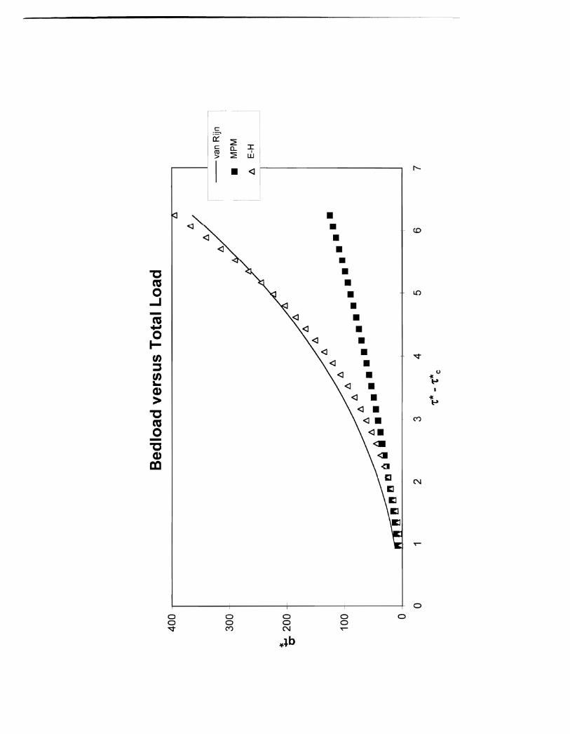
b. Van Rijn (1984 a,b).

From an extensive empirical analysis of field data, Van Rijn developed a complex empirical relation for total load in sandy systems that in practice is similar to Engelund and Hansen’s simple relation, but is more general. His relations must be implemented in a spreadsheet and one can be made available to you. Also, it is worth noting that Van Rijn’s relations can be closely matched with a form similar to the Meyer-Peter Mueller bedload relation, where the excess shear stress is raised to a power in the range 1.8 – 2.5, depending on conditions.

Powerpoint graph comparing bedload and suspended load flux.

7

Dimensional Data

0.00E+00 1.00E+01 2.00E+01 3.00E+01 4.00E+01 5.00E+01 6.00E+01

0.00E+0 0

1.00E+0 1

2.00E+0 1

3.00E+0 1

4.00E+0 1

5.00E+0 1

Shear Stress (Pa)

/s)

1 cm, qtz 4 cm, coal 2 cm, qtz 3 cm, glycerin

Dimensional Data

y = 0.0003x3.1545

R2 = 0.755

0.00E+00 1.00E+01 2.00E+01 3.00E+01 4.00E+01 5.00E+01 6.00E+01

0.00E+0 0

1.00E+0 1

2.00E+0 1

3.00E+0 1

4.00E+0 1

5.00E+0 1

Shear Stress (Pa)

/s)

Series1 Power (Series1)

Dimensionless Data

0

0.1

0.2

0.3

0.4

0.5

0.00E+00 5.00E-02 1.00E-01 1.50E-01 2.00E-01 2.50E-01

Shields Stress

1 cm, qtz 4 cm, coal 2 cm, qtz 3 cm, glycerin

Sed

Flux

(cm

^2

Sed

Flux

(cm

^2N

on-d

Sed

Flu

x

GRAIN SIZE SCALES FOR SEDIMENTS

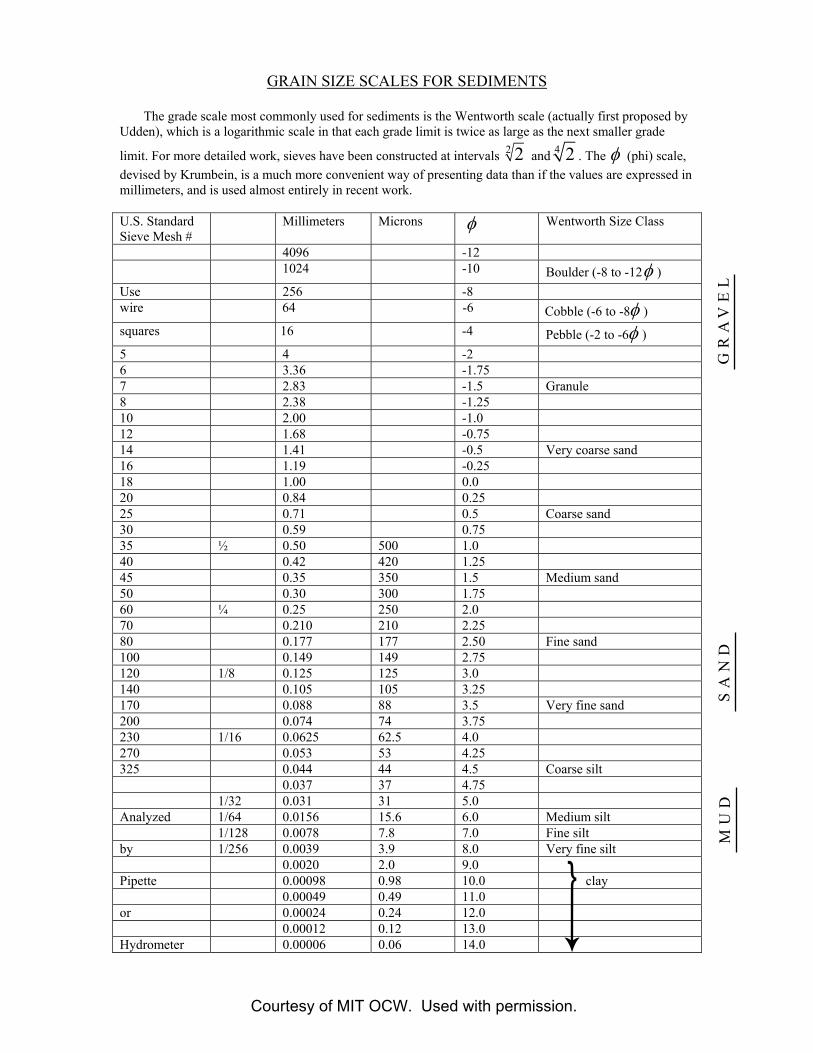
The grade scale most commonly used for sediments is the Wentworth scale (actually first proposed by Udden), which is a logarithmic scale in that each grade limit is twice as large as the next smaller grade

limit. For more detailed work, sieves have been constructed at intervals 2 2 and 4 2 . The φ (phi) scale, devised by Krumbein, is a much more convenient way of presenting data than if the values are expressed in millimeters, and is used almost entirely in recent work.

U.S. Standard Sieve Mesh #

Millimeters Microns φ Wentworth Size Class

4096 -12 1024 -10 Boulder (-8 to -12φ )

Use 256 -8 wire 64 -6 Cobble (-6 to -8φ ) squares 16 -4 Pebble (-2 to -6φ ) 5 4 -2 6 3.36 -1.75 7 2.83 -1.5 Granule 8 2.38 -1.25 10 2.00 -1.0 12 1.68 -0.75 14 1.41 -0.5 Very coarse sand 16 1.19 -0.25 18 1.00 0.0 20 0.84 0.25 25 0.71 0.5 Coarse sand 30 0.59 0.75 35 1⁄2 0.50 500 1.0 40 0.42 420 1.25 45 0.35 350 1.5 Medium sand 50 0.30 300 1.75 60 1⁄4 0.25 250 2.0 70 0.210 210 2.25 80 0.177 177 2.50 Fine sand 100 0.149 149 2.75 120 1/8 0.125 125 3.0 140 0.105 105 3.25 170 0.088 88 3.5 Very fine sand 200 0.074 74 3.75 230 1/16 0.0625 62.5 4.0 270 0.053 53 4.25 325 0.044 44 4.5 Coarse silt

0.037 37 4.75 1/32 0.031 31 5.0 Analyzed 1/64 0.0156 15.6 6.0 Medium silt

1/128 0.0078 7.8 7.0 Fine silt by 1/256 0.0039 3.9 8.0 Very fine silt

0.0020 2.0 9.0 Pipette 0.00098 0.98 10.0 clay

0.00049 0.49 11.0 or 0.00024 0.24 12.0

0.00012 0.12 13.0 Hydrometer 0.00006 0.06 14.0

MU

D

SA

ND

G

RA

VE

L

Courtesy of MIT OCW. Used with permission.

Image courtesy of USGS.

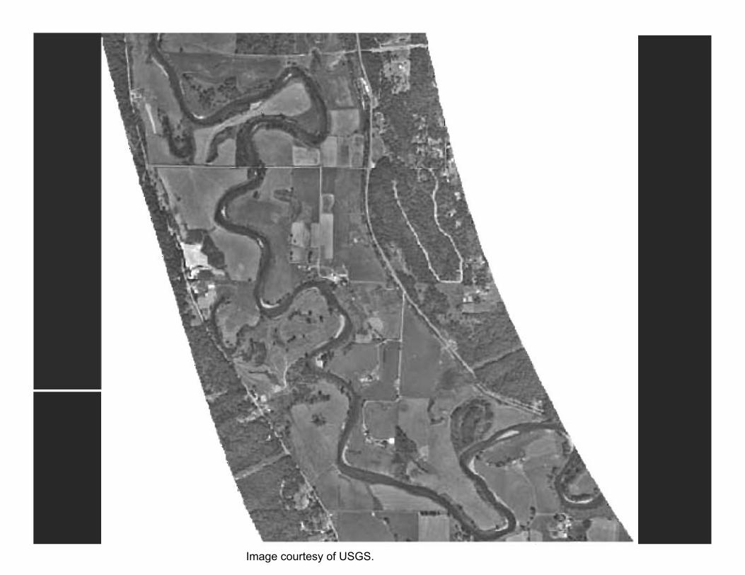
Image courtesy of USGS.

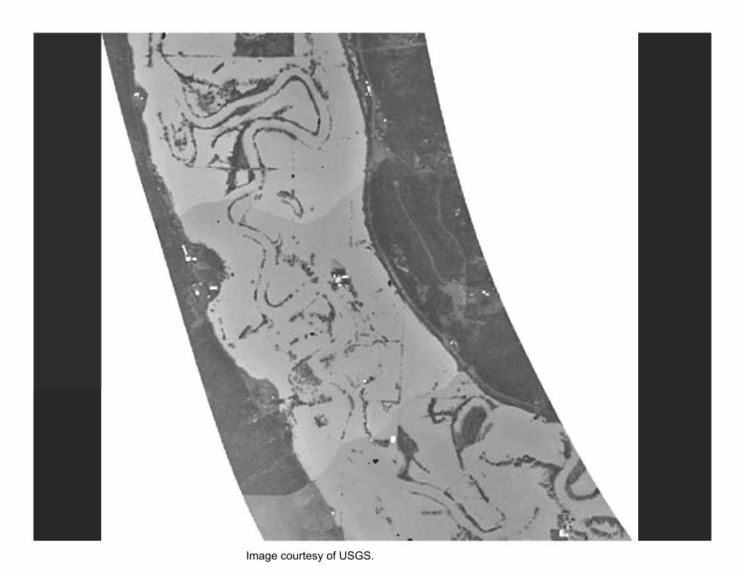
Image courtesy of USGS.

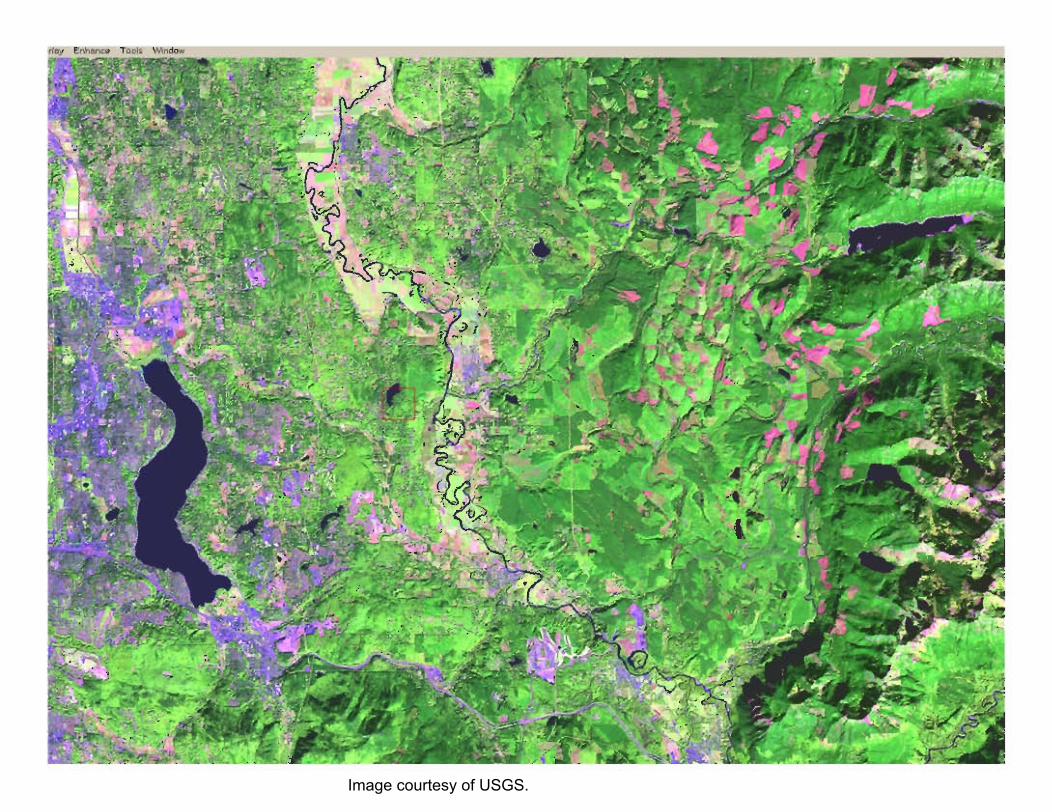
Image courtesy of USGS.