高等輸送二 — 質傳

Lecture 3Dispersion

郭修伯 助理教授

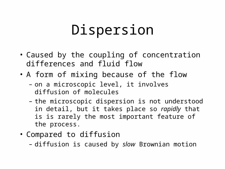
Dispersion

• Caused by the coupling of concentration differences and fluid flow

• A form of mixing because of the flow– on a microscopic level, it involves diffusion of molecules

– the microscopic dispersion is not understood in detail, but it takes place so rapidly that is is rarely the most important feature of the process.

• Compared to diffusion– diffusion is caused by slow Brownian motion

Smoke pouring from a smokestack

Affected by wind, weather, and different amounts of smoke

Qualitatively similar to diffusion: the concentration profile is a Gaussian profile.From our previous calculation on a sharp pulse of solute:

Dt

y

eDtA

Mc

4

1

2

4

tE

y

y

ye

vx

E

c 4

0

1

2

1

Speed of windDispersion coefficient (L2/t)

Dispersion coefficient

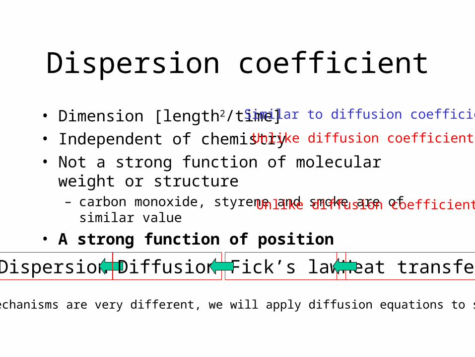
• Dimension [length2/time]

• Independent of chemistry

• Not a strong function of molecular weight or structure– carbon monoxide, styrene and smoke are of similar value

• A strong function of position

Similar to diffusion coefficient

Unlike diffusion coefficient

Unlike diffusion coefficient

Dispersion Diffusion Fick’s law Heat transfer

Although the mechanisms are very different, we will apply diffusion equations to study dispersion

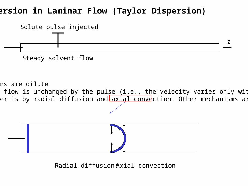
Dispersion in Laminar Flow (Taylor Dispersion)

Solute pulse injected

z

Steady solvent flow

Assumption:• the solutions are dilute• the laminar flow is unchanged by the pulse (i.e., the velocity varies only with radius)• mass transfer is by radial diffusion and axial convection. Other mechanisms are neglected.

Radial diffusion Axial convection

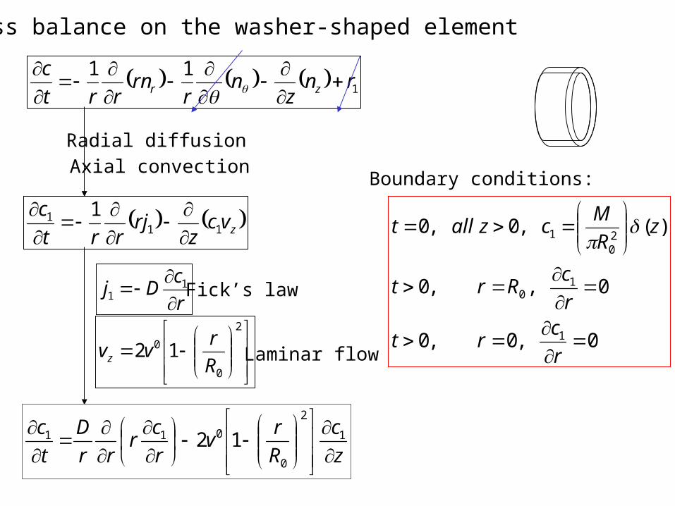
A mass balance on the washer-shaped element

1

11rn

zn

rrn

rrt

czr

Radial diffusionAxial convection

zvcz

rjrrt

c11

1 1

r

cDj

11 Fick’s law

2

0

0 12R

rvvz Laminar flow

z

c

R

rv

r

cr

rr

D

t

c

1

2

0

011 12

Boundary conditions:

0,0,0

0,,0

)(,0,0

1

10

20

1

r

crt

r

cRrt

zR

Mczallt

z

c

R

rv

r

cr

rr

D

t

c

1

2

0

011 12

0,0,0

0,,0

)(,0,0

1

10

20

1

r

crt

r

cRrt

zR

Mczallt

0R

r

0

0 )(

R

tvz

12

001

2

12

cRv

cD

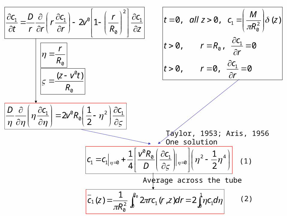
Taylor, 1953; Aris, 1956One solution

42

010

0

011 2

1

4

1 c

D

Rvcc

1

0 10 120

1 2),(21

)(0

dcdrzrrc

Rzc

R

Average across the tube

(1)

(2)

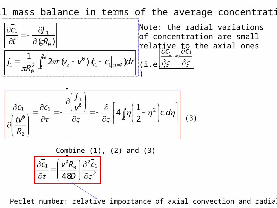
An overall mass balance in terms of the average concentration:

)( 0

11

R

J

t

c

Note: the radial variations of concentration

are small relative to the axial ones

(i.e., )

11 cc

0

0 0110

20

1 ))((21 R

z drccvvrR

j

1

0 12

01

1

0

0

1

2

14

dc

vJ

c

Rtv

c(3)

Combine (1), (2) and (3)

2

12

00

1

48

c

D

Rvc

Peclet number: relative importance of axial convection and radial diffusion

2

12

00

1

48

c

D

Rvc

0,0,0

0,,0

)(,0,0

1

1

30

1

ct

c

R

Mcall

tE

tvz

z

zetE

RMc 4

)(20

1

20

4

D

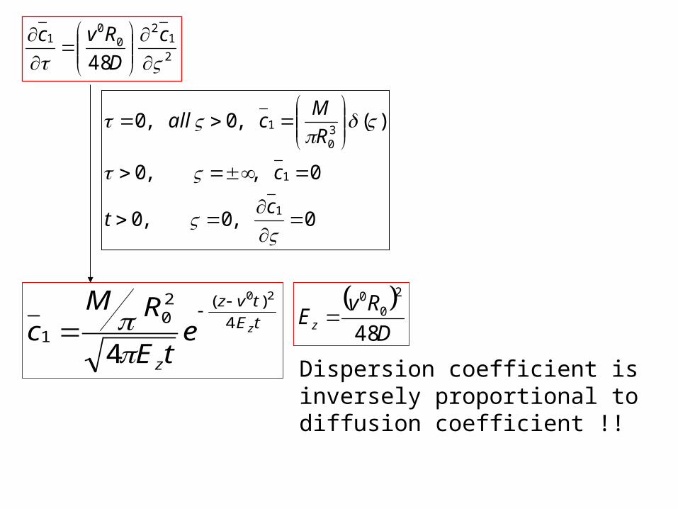
RvEz 48

2

00

Dispersion coefficient is inversely proportional to diffusion coefficient !!

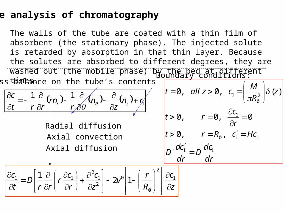
The analysis of chromatography

The walls of the tube are coated with a thin film of absorbent (the stationary phase). The injected solute is retarded by absorption in that thin layer. Because the solutes are absorbed to different degrees, they are washed out (the mobile phase) by the bed at different times.

A mass balance on the tube’s contents

1

11rn

zn

rrn

rrt

czr

Radial diffusionAxial convection

z

c

R

rv

z

c

r

cr

rrD

t

c

1

2

0

021

211 12

1

Axial diffusion

Boundary conditions:

dr

dcD

dr

cdD

HccRrtr

crt

zR

Mczallt

11

110

1

20

1

,,0

0,0,0

)(,0,0

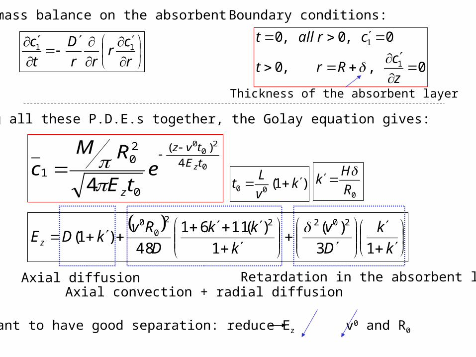
A mass balance on the absorbent

r

cr

rr

D

t

c 11

Boundary conditions:

0,,0

0,0,0

1

1

z

cRrt

crallt

Thickness of the absorbent layer

Solving all these P.D.E.s together, the Golay equation gives:

0

20

0

4

)(

0

20

14

tE

tvz

z

zetE

RMc

k

k

D

v

k

kk

D

RvkDEz 13

)(

1

)(1161

48)1(

20222

00

)1(00 k

v

Lt

0R

Hk

Axial diffusionAxial convection + radial diffusion

Retardation in the absorbent layer

We want to have good separation: reduce Ez v0 and R0

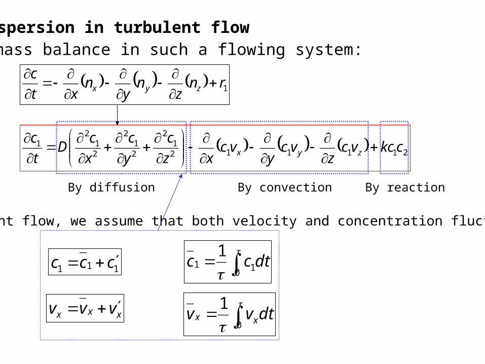
Dispersion in turbulent flowThe mass balance in such a flowing system:

1rnz

ny

nxt

czyx

2111121

2

21

2

21

21 ckcvc

zvc

yvc

xz

c

y

c

x

cD

t

czyx

By diffusion By convection By reaction

In turbulent flow, we assume that both velocity and concentration fluctuate:

111 ccc

0 111

dtcc

xxx vvv

0

1dtvv xx

2121111

1112

12

2

12

2

12

1

cckcckvcz

vcy

vcx

vcz

vcy

vcxz

c

y

c

x

cD

t

c

zyx

zyx

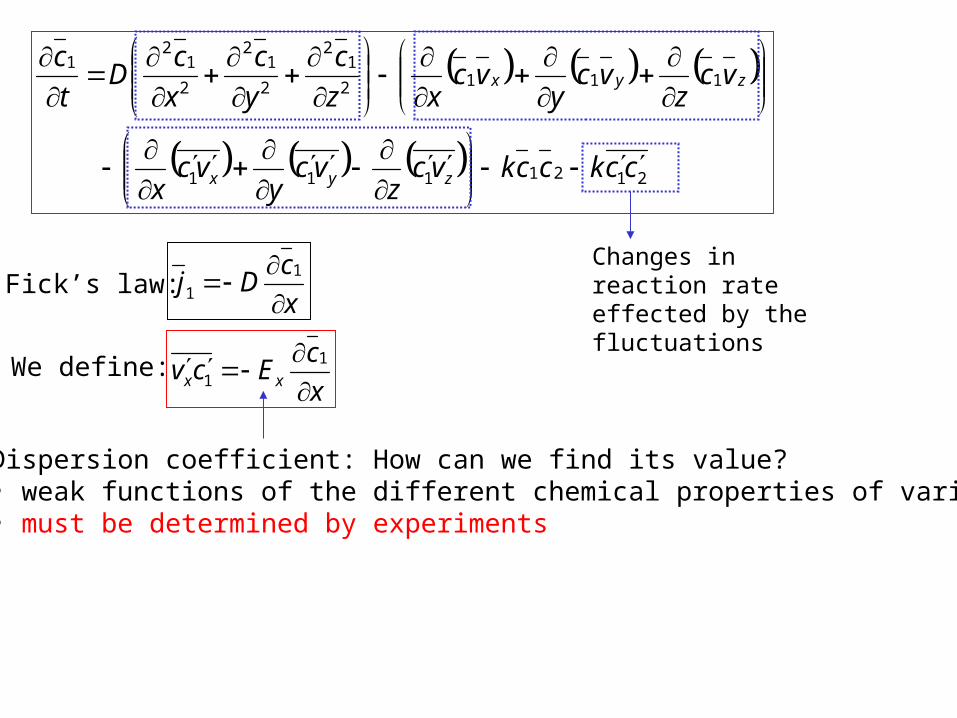
Changes in reaction rate effected by the fluctuations

x

cDj

1

1

We define:x

cEcv xx

1

1

Fick’s law:

Dispersion coefficient: How can we find its value?• weak functions of the different chemical properties of various solute• must be determined by experiments

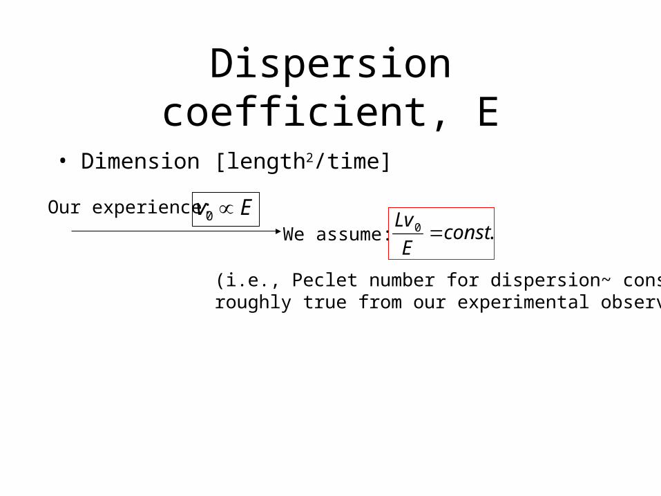
Dispersion coefficient, E

• Dimension [length2/time]

.0 constE

Lv

(i.e., Peclet number for dispersion~ constant)roughly true from our experimental observation

Ev 0Our experience:

We assume:

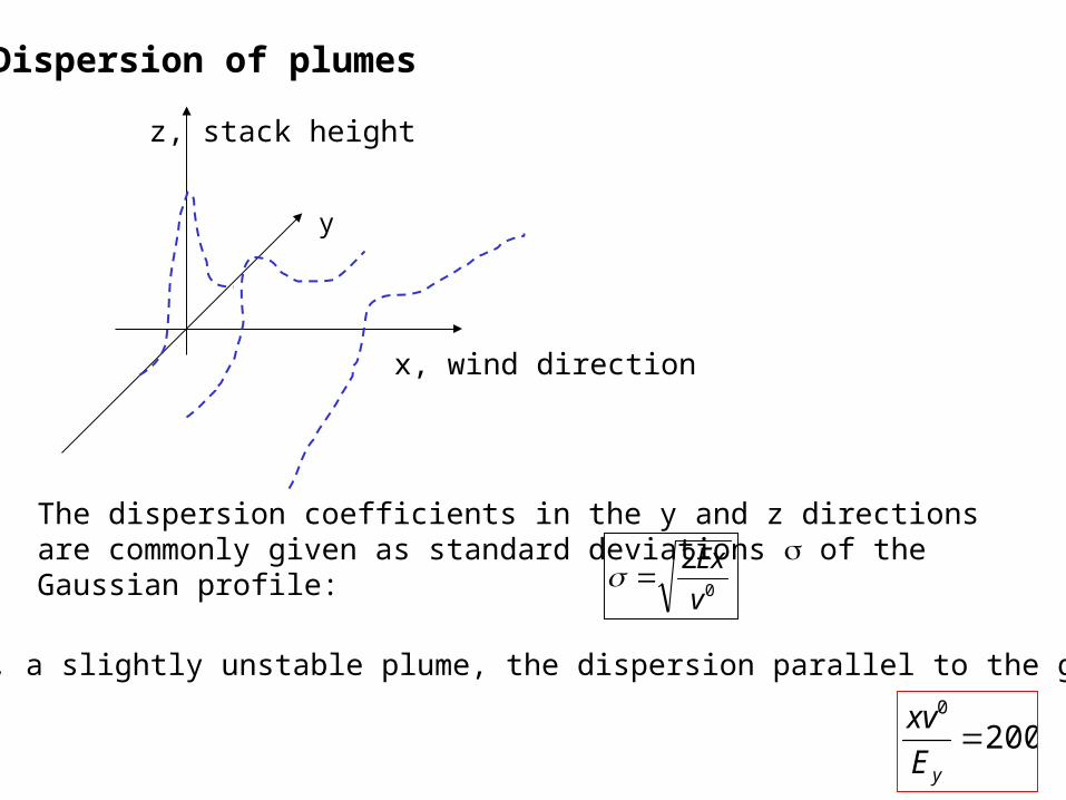
Dispersion of plumes

x, wind direction

z, stack height

The dispersion coefficients in the y and z directions are commonly given as standard deviations of the Gaussian profile:

0

2

v

Ex

y

For example, a slightly unstable plume, the dispersion parallel to the ground is:

2000

yE

xv

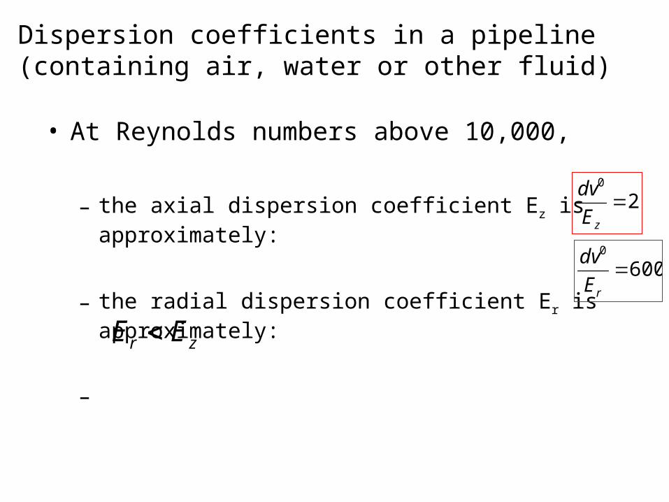
Dispersion coefficients in a pipeline (containing air, water or other fluid)

20

zE

dv

• At Reynolds numbers above 10,000,

– the axial dispersion coefficient Ez is approximately:

– the radial dispersion coefficient Er is approximately:

–

6000

rE

dv

zr EE

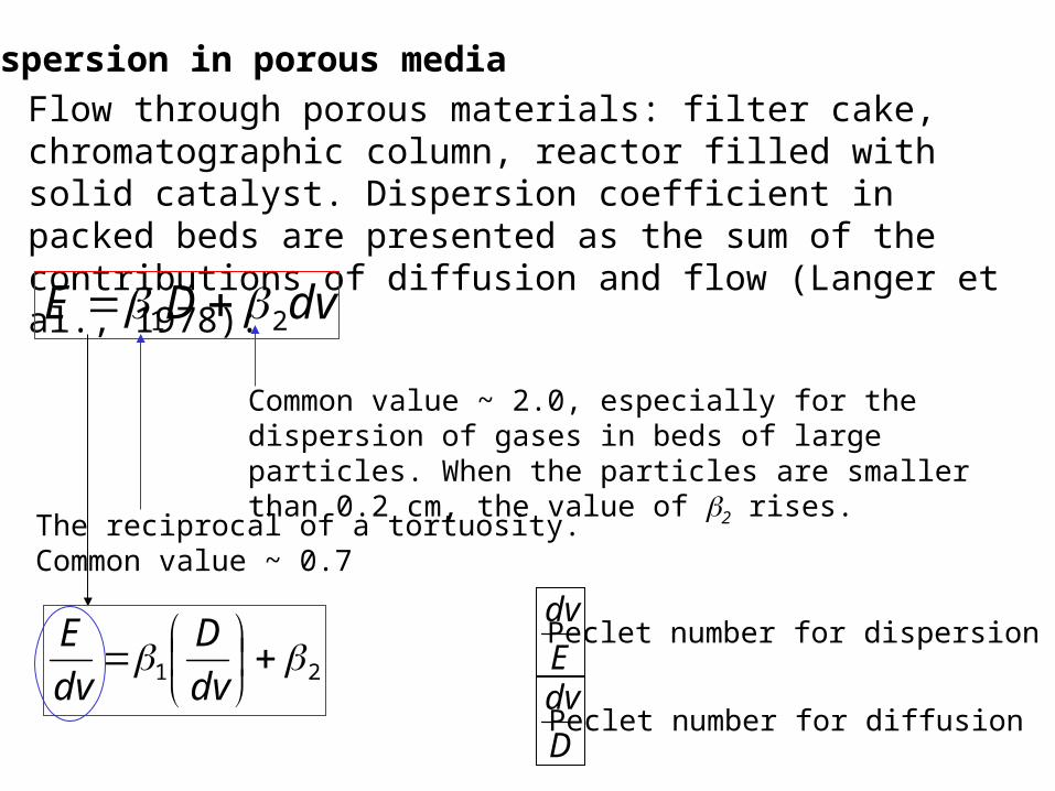
Dispersion in porous media

Flow through porous materials: filter cake, chromatographic column, reactor filled with solid catalyst. Dispersion coefficient in packed beds are presented as the sum of the contributions of diffusion and flow (Langer et al., 1978):

dvDE 21

The reciprocal of a tortuosity.Common value ~ 0.7

Common value ~ 2.0, especially for the dispersion of gases in beds of large particles. When the particles are smaller than 0.2 cm, the value of 2 rises.

21

dv

D

dv

EE

dvPeclet number for dispersion

D

dvPeclet number for diffusion

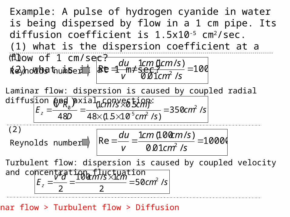
Example: A pulse of hydrogen cyanide in water is being dispersed by flow in a 1 cm pipe. Its diffusion coefficient is 1.5x10-5 cm2/sec.(1) what is the dispersion coefficient at a flow of 1 cm/sec?(2) what is it at 1 m/sec?(1)

Reynolds number 100/01.0

)/1(1Re

2

scm

scmcm

v

du

Laminar flow: dispersion is caused by coupled radial diffusion and axial convection:

scm

scm

cmscm

D

RvEz /350

)/105.1(48

)5.0/1(

482

25

22

00

(2)

Reynolds number 10000/01.0

)/100(1Re

2

scm

scmcm

v

du

Turbulent flow: dispersion is caused by coupled velocity and concentration fluctuation

scmcmscmdv

Ez /502

1/100

22

0

Laminar flow > Turbulent flow > Diffusion

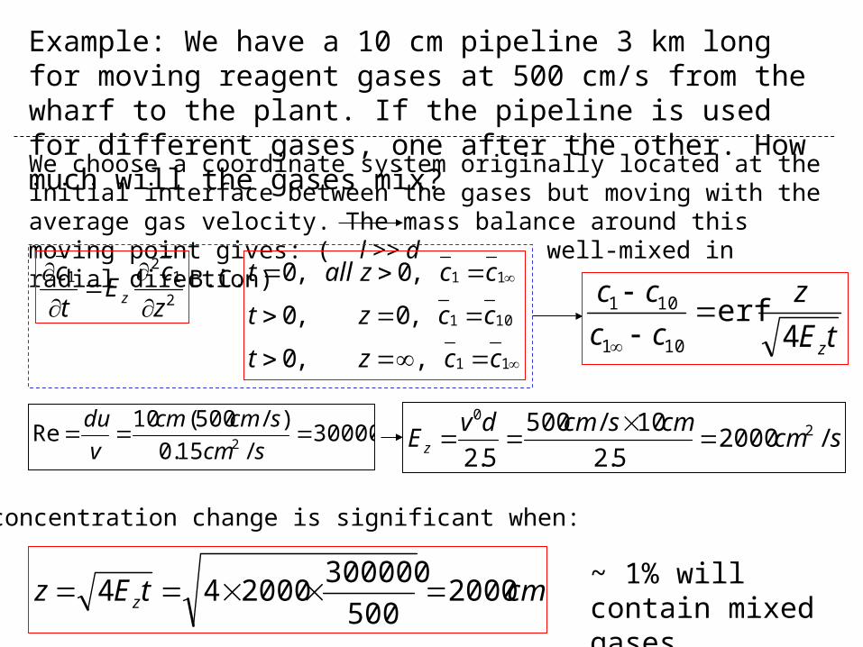
Example: We have a 10 cm pipeline 3 km long for moving reagent gases at 500 cm/s from the wharf to the plant. If the pipeline is used for different gases, one after the other. How much will the gases mix?We choose a coordinate system originally located at the initial interface between the gases but moving with the average gas velocity. The mass balance around this moving point gives: ( l >> d well-mixed in radial direction)

2

12

1

z

cE

t

cz

B.C.

11

101

11

,,0

,0,0

,0,0

cczt

cczt

cczallt

tE

z

cc

cc

z4erf

101

101

30000/15.0

)/500(10Re

2

scm

scmcm

v

duscm

cmscmdvEz /2000

5.2

10/500

5.22

0

The concentration change is significant when:

cmtEz z 2000500

300000200044 ~ 1% will contain

mixed gases