Japan Advanced Institute of Science and Technology

JAIST Repositoryhttps://dspace.jaist.ac.jp/

Title矩形パッキングとそのVLSIモジュール配置問題への応

用

Author(s) 村田, 洋

Citation

Issue Date 1997-03

Type Thesis or Dissertation

Text version author

URL http://hdl.handle.net/10119/833

Rights

Description Supervisor:岡本 栄司, 情報科学研究科, 博士

Rectangle Packing and Its Applications to

VLSI Module Placement Problem

By Hiroshi Murata

A thesis submitted to

School of Information Science,

Japan Advanced Institute of Science and Technology,

in partial ful�llment of the requirements

for the degree of

Doctor of Information Science

Graduate Program in Information Science

Written under the direction of

Professor Eiji Okamoto

January 16, 1997

Copyright c 1997 by Hiroshi MURATA

Abstract

The �rst and the most critical stage in VLSI layout design is the placement. Its

background is the rectangle packing problem : Given a set of rectangular modules of ar-

bitrary sizes, place them without overlap on a plane within a rectangle of the minimum

area. Since the variety of the packing is uncountably in�nite, the key issue for success-

ful optimization is the introduction of a �nite solution space which includes an optimal

solution and excludes all the infeasible solutions. The main contribution of this thesis is

in the introduction of such a solution space where each packing is represented by a pair

of module name sequences, called sequence-pair. The introduction of this solution space

enables us to use stochastic optimization method such as simulated annealing, and it is

demonstrated that hundreds of modules was packed very e�ciently. The biggest MCNC

benchmark example is also shown to be placed very promisingly with a conventional wiring

consideration method.

Although module positions are successfully represented by the sequence-pair, it is

desired frequently in VLSI design that channels are represented together with modules,

because a channel router is often used in the following routing stage. For this request, this

thesis gives a mapping from a sequence-pair to a rectangular dissection, which represents

channels by line segments.

Placement with obstacles in the chip is also discussed in this thesis, for dealing with

pre-placed modules and with a rectilinear placement region. The obstacles are easily

included in a sequence-pair to eliminate the overlaps, but the sequence-pair cannot guar-

antee to recover the assigned coordinates of the obstacles. To solve this practical problem,

this thesis gives an algorithm which changes an inconsistent sequence-pair to a consistent

one.

i

Acknowledgments

The author indebted to his principal advisor Professor Eiji Okamoto of Japan Ad-

vanced Institute of Science and Technology for his constant encouragement.

The author would like to thank to his advisor Associate Professor Kunihiko Hiraishi

of Japan Advanced Institute of Science and Technology for his helpful discussions and

suggestions.

Special thanks are to Associate Professor Mineo Kaneko of Japan Advanced Institute

of Science and Technology for his constant guidance. Much of the �nal year of research

was guided by him.

The author wishes to express his sincere gratitude to his prior principal advisor Pro-

fessor Yoji Kajitani of Tokyo Institute of Technology for his helpful discussions, guidance,

and all the activities, that inspired the author throughout the course of this research.

The author devotes his sincere thanks and appreciation to Research Associate Ku-

nihiro Fujiyoshi of Japan Advanced Institute of Science and Technology, currently at

Tokyo University of Agriculture and Technology. His eager discussions helped the author

especially on building the proofs presented in this thesis.

Special thanks are to Research Associate Shigetoshi Nakatake of Tokyo Institute of

Technology. He jointly started this research with the author, and has been an excellent

partner throughout the research. He gave the �rst idea for our common target, and the

discussions on his initial idea helped the author to develop the theory presented in this

thesis.

The author is grateful to all who have a�ected or suggested his areas of research,

especially to Visiting Professor Milan Vlach and Visiting Associate Professor Magnus

Halld�orsson.

Special thanks are to Mr. Eda, Mr. Funahara, Mr. Kaneko, Mr. Yamagishi and all

the engineers at Murata Mfg., Co. Ltd. The motivation of this research is mainly from

the author's experience in developing the CAD/FA system with them.

Finally, I would like to thank my wife Akiko and our sons Shun'ichi and Tatsurou for

their love and support.

ii

Contents

Abstract i

Acknowledgments ii

1 Introduction 1

1.1 Rectangle Packing Problem : : : : : : : : : : : : : : : : : : : : : : : : : : 1

1.2 Previous Researches : : : : : : : : : : : : : : : : : : : : : : : : : : : : : : 1

1.3 Thesis Outline : : : : : : : : : : : : : : : : : : : : : : : : : : : : : : : : : : 2

1.4 Remarks : : : : : : : : : : : : : : : : : : : : : : : : : : : : : : : : : : : : : 3

2 Rectangle Packing Solution Space Composed of Sequence-Pairs 4

2.1 Introduction : : : : : : : : : : : : : : : : : : : : : : : : : : : : : : : : : : : 4

2.2 From Packing to Sequence-Pair : : : : : : : : : : : : : : : : : : : : : : : : 6

2.2.1 Gridding : : : : : : : : : : : : : : : : : : : : : : : : : : : : : : : : : 6

2.2.2 Geometrical Information of Sequence-Pair : : : : : : : : : : : : : : 9

2.3 From Sequence-Pair to Packing : : : : : : : : : : : : : : : : : : : : : : : : 10

2.3.1 Constraint of Sequence-Pair : : : : : : : : : : : : : : : : : : : : : : 10

2.3.2 Best Packing Under the Constraint : : : : : : : : : : : : : : : : : : 10

2.3.3 P-admissible Solution Space : : : : : : : : : : : : : : : : : : : : : : 11

2.4 Use of Sequence-Pair : : : : : : : : : : : : : : : : : : : : : : : : : : : : : : 13

2.4.1 Rectangle Packing : : : : : : : : : : : : : : : : : : : : : : : : : : : 13

2.4.2 Module Placement with Wires : : : : : : : : : : : : : : : : : : : : : 14

2.5 Conclusion : : : : : : : : : : : : : : : : : : : : : : : : : : : : : : : : : : : : 16

3 Mapping from Sequence-Pair to Rectangular-Dissection 18

3.1 Introduction : : : : : : : : : : : : : : : : : : : : : : : : : : : : : : : : : : : 18

3.2 Preliminary : : : : : : : : : : : : : : : : : : : : : : : : : : : : : : : : : : : 19

3.2.1 HV-Relation-Set : : : : : : : : : : : : : : : : : : : : : : : : : : : : 19

3.2.2 Sequence-Pair : : : : : : : : : : : : : : : : : : : : : : : : : : : : : : 19

3.2.3 Rectangular-Dissection : : : : : : : : : : : : : : : : : : : : : : : : : 21

3.2.4 Sequence-Pair and Rectangular-Dissection : : : : : : : : : : : : : : 22

3.3 Rectangular-Dissection without Empty Room : : : : : : : : : : : : : : : : 24

3.3.1 HV-Cross and Adjacent-Cross : : : : : : : : : : : : : : : : : : : : : 24

3.3.2 Converting Sequence-Pair into Rectangular-Dissection : : : : : : : : 25

3.3.3 Necessary and Su�cient Condition : : : : : : : : : : : : : : : : : : 29

3.4 Rectangular-Dissection with Fewest Empty Rooms : : : : : : : : : : : : : 30

3.4.1 Removing Adjacent-Crosses : : : : : : : : : : : : : : : : : : : : : : 30

3.4.2 Maximum Number of Empty Rooms : : : : : : : : : : : : : : : : : 33

iii

3.5 Conclusion : : : : : : : : : : : : : : : : : : : : : : : : : : : : : : : : : : : : 33

4 Rectangle Packing with Obstacles 35

4.1 Introduction : : : : : : : : : : : : : : : : : : : : : : : : : : : : : : : : : : : 35

4.2 Preliminary : : : : : : : : : : : : : : : : : : : : : : : : : : : : : : : : : : : 36

4.2.1 Rectangle Packing with Pre-Placed Rectangles (RPP) : : : : : : : : 36

4.2.2 Sequence-Pair : : : : : : : : : : : : : : : : : : : : : : : : : : : : : : 36

4.2.3 Feasibility of Sequence-Pair : : : : : : : : : : : : : : : : : : : : : : 38

4.3 Adaptation : : : : : : : : : : : : : : : : : : : : : : : : : : : : : : : : : : : 40

4.3.1 Necessary Condition : : : : : : : : : : : : : : : : : : : : : : : : : : 40

4.3.2 Algorithm : : : : : : : : : : : : : : : : : : : : : : : : : : : : : : : : 41

4.3.3 Illustrative Example : : : : : : : : : : : : : : : : : : : : : : : : : : 41

4.3.4 Proof of Adaptation : : : : : : : : : : : : : : : : : : : : : : : : : : 43

4.4 Use of Adaptation : : : : : : : : : : : : : : : : : : : : : : : : : : : : : : : 45

4.4.1 RPP Example : : : : : : : : : : : : : : : : : : : : : : : : : : : : : : 45

4.4.2 Place and Route Example : : : : : : : : : : : : : : : : : : : : : : : 47

4.5 Conclusion : : : : : : : : : : : : : : : : : : : : : : : : : : : : : : : : : : : : 48

5 Conclusion 49

References 50

Publications 52

iv

Chapter 1

Introduction

1.1 Rectangle Packing Problem

Layout in physical design of VLSI is, simply to say, to pack all the circuit elements in a chip

without violating the design rules, so that the circuit performs well and the production

yield is high. Among the variety of targets in di�erent stages, the problem de�ned as

follows is the base of all of them.

Rectangle Packing Problem: RP

LetM be a set of n rectangular modules whose heights and widths are given in

real numbers. (Orientations are �xed.) A packing ofM is a non-overlapping

placement of all the modules. The minimum bounding rectangle of a packing

is called the chip. Find a packing ofM in a chip of the minimum area.

Notice that RP is not simply a combinatorial optimization problem since the heights

and widths of modules are arbitrary real numbers. It will be shown in this thesis that the

problem belongs to the NP-hard class.

1.2 Previous Researches

Similar problems have been studied from mathematical interests [1, 2, 3, 4, 5], but they

are far from real applications in VLSI layout design. In VLSI design, deterministic algo-

rithms have been used based on heuristic ideas [6, 7], but they easily fall in a non-global

local-optimum. An alternative approach is to use stochastic searches, such as simulated

annealing and genetic algorithm. A stochastic search is known to have a potential for

�nding one of the best solutions in the \solution space" in a controlled time [8, 9].

To apply a stochastic search, it is required to reduce the problem into a combinatorial

level by introducing a discrete solution space. A solution space is a set of codes, each

of which represents a construction of placement. A stochastic search is to explore the

solution space randomly and heuristically to �nd a good solution, and to output the best

found solution by the end of the given limit of time. However, if the solution space does

not include any optimal solution, the found solution cannot be optimal. Unfortunately,

an optimal solution is not guaranteed to be included in the most of known solution

spaces [10, 11, 12]. The solution space proposed by Onodera, Taniguchi and Tamaru [13]

includes an optimal solution but also includes infeasible solutions, thus it is not useful

1

for a stochastic search. (They uses an exhaustive algorithm, but the size of the tractable

problem is limited up to six modules.)

The discussion above concludes that the key issue is to invent a solution space which

includes an optimal solution but excludes all the infeasible solutions. Such a solution

space is said to be P -admissible in this research, though there is no known example for

the rectangle packing problem.

1.3 Thesis Outline

The main contribution of this thesis is �nding a P -admissible solution space for the rect-

angle packing problem. The solution space is de�ned as follows. A pair of module name

sequences (for example, (abcd; bdac) for modules a; b; c and d) is called a sequence-pair. It

is de�ned that sequence-pair implies a horizontal/vertical (right of, left of, below, above)

relation for every pair of modules m and m0, depending on whether m is fbefore, afterg

m0in the f�rst, secondg sequence. A compaction procedure is given so that it makes a

sequence-pair corresponds to a best packing of all the packings that satisfy the implied hor-

izontal/vertical relations. The set of all the sequence-pairs, thus of the cardinality (n!)2,

is our solution space. The P -admissibility of this solution space is proved in detail in

this thesis. In experiments using the data abstracted from industrial examples, hundreds

of modules are e�ectively packed. Furthermore, to see how the method is promising, an

example of tens of modules is shown to be placed with a conventional wiring consideration

method.

A sequence-pair represents a non-overlapping placement of modules, but by nature it

does not represent any wiring channel. This could be a di�culty in applying the method to

IC layout in which the placement is followed by a channel router. In previous researches,

a rectangular dissection has been used to represent relative positions of channels as well

as relative positions of modules. As a complementary contribution to the sequence-pair

method, we give a mapping from a sequence-pair to a rectangular dissection, introducing

the minimum number of channels to preserve the information on module positions. The

tight upper bound of the number of introduced channels is given with detailed proofs.

As a practical contribution of this thesis, further consideration is devoted to cope with

a speci�c requirement in PCB/VLSI design. In typical PCBs, there are obstacles such

as holes and connectors. The obstacles are often found also in VLSI design, for example,

pre-placed macro cells. To eliminate the modules being overlapped with such obstacles,

these obstacles can be modeled as \pre-placed modules" and included in a sequence-

pair. However, it is not guaranteed that such a sequence-pair can recover the assigned

coordinates of the pre-placed modules. A procedure is presented to change an arbitrary

sequence-pair to �t such environments.

This thesis is organized as follows. In Chapter 2, the sequence-pair is introduced

and its P -admissibility is proved. In Chapter 3, a mapping from a sequence-pair to a

rectangular-dissection is provided to generate channel information. Chapter 4 is devoted

to present an adaptation procedure to tailor the solution space for the obstacles. Finally,

Chapter 5 concludes this research with remarks.

2

1.4 Remarks

The Sequence-Pair idea was born in a research discussion in Kajitani-lab, Japan Advanced

Institute of Science and Technology, in 1994, inspired by another idea, called Bounded-

Sliceline-Grid (BSG), which is a uniform grid structure but specially designed for VLSI

module placement problems. Since then, they have been working together to develop the

BSG method and the Sequence-Pair method in parallel, as is listed in the publications

section. However, this thesis rarely describes about BSG method, since theory of the

sequence-pair is discussed in a complete and closed form. The birth and growth of the

BSG and the Sequence-Pair in the very early stage are described in [15] which was written

by the then Advisor Professor Y. Kajitani.

3

Chapter 2

Rectangle Packing Solution Space

Composed of Sequence-Pairs

2.1 Introduction

Layout in physical design of VLSI is, in short, to pack all the circuit elements in a chip

without violating design rules, so that the circuit performs well and the production yield

is high. There are so much variety of targets in di�erent stages but the following problem

is the core of them.

Rectangle Packing Problem: RP

LetM be a set of n rectangular modules of �xed orientations, whose heights and widths

are given in real numbers. A packing ofM is a non-overlapping placement of the modules.

The minimum bounding rectangle of a packing is called the chip. Find a packing of Monto a chip of the minimum area.

A packing of six modules is shown in Fig. 2.1.

The decision version of our problem RP(A) is to decide whether M can be packed

onto a chip of area A. Baker, Co�man and Rivest [1] proved the NP-completeness of asimilar problem RP(H,W) : decide whetherM can be packed onto the chip of height H

and width W . We can show RP(A) to be NP-complete using the fact that any instanceof RP(H,W) can be polynomially reducible to an instance of RP(A) by the following

conversion.

r the maximum width over modules

2HA (W + rH)(W + 2rH)

M0 f (w � rh) j 8 (w � h) 2 Mg [ f rH � rH ; (W + rH)� (W + rH) gOur problem RP is harder than RP(A), so NP-hard.

Since the heights and widths of modules are real numbers, RP is not simply a combina-

torial optimization problem. In fact, there have been several numerical approaches [6, 7].

They �rst generate a possibly overlapping arrangement of modules, and then move mod-

ules to reduce the overlapping cost. But the overlap elimination is very hard for the

numerical approaches without ad-hoc post-processing.

An alternative approach is \combinatorial search". In this approach, a set of codes is

de�ned as a solution space. Each code represents a construction of placement. A code is

4

said to be feasible if the construction is consistent, i.e. there exists a packing corresponding

to the code. The evaluation of a feasible code is the area of the chip, and the evaluation

of an infeasible code is in�nitely negative. The combinatorial search aims at �nding a

best code in the solution space. However, exhaustive search of the whole space will take

too much time. Since the problem is NP-hard, the size of any such solution space is

expected to be exponential. Several heuristics have been proposed to �nd a good solution

in a moderate time, for example, simulated annealing and genetic algorithms. Given a

time limit, such a heuristic stops the search half-way and outputs the best solution found

so far. For this search to be e�ective, the minimum requirement of the solution space is

the following four items.

(1) The solution space is �nite.

(2) Every solution is feasible.

(3) Realization of a code is possible in polynomial time.

(4) There exists a code which corresponds to one of the optimal solutions.

The solution space that satis�es the above four requirements is called P-admissible.

The reasons for (1),(3) and (4) are obvious. That for (2) is: most heuristics pick up

one solution after another along the neighboring structure de�ned on the space, consulting

with the di�erence of evaluations (gain) to the previous solution. Therefore, if infeasible

solutions are included, the continuity will be destroyed and convergence to a feasible

solution is not guaranteed.

A known practical solution space is one derived from the slicing oorplan proposed

by Otten [10] and others. It satis�es (1), (2) and (3). Several optimization heuristics are

applied for the space, and one of the most successful approaches uses simulated anneal-

ing [8]. However, since the optimal solution can be non-slicing, (4) is not satis�ed. This

fact discourages us to start searching for the best in the space. E�orts have been paid to

let the space include non-slicing structures [12, 11], but they have not been successful to

satisfy (4). (Still, a merit of the slicing structure is in the channel routing stage [16].)

Another approach is proposed by Onodera, Taniguchi and Tamaru [13]. They con-

struct a solution space by assigning one out of the four relations, \left of", \right of",

\above", and \below", to every pair of modules. This space satis�es (4) since any packing

satis�es a combination of the relations. But there are many infeasible codes such as; mod-

ule a is left of module b, b is left of c and c is left of a. Thus their space is not P-admissible

either. As a consequence, the space does not admit heuristics such as simulated annealing.

In their paper, exhaustive search with a branch-and-bound technique is applied to �nd an

exactly optimal solution, but the size of tractable problems is limited up to six modules.

This chapter provides a P-admissible solution space, in which each code is a pair of

module name sequences. By searching this space, it has become possible to pack hundreds

of modules e�ciently, as demonstrated in Fig. 2.9 and Fig. 2.10.

To utilize this solution space of RP for VLSI layout design, the evaluation of a packing

has to be modi�ed to consider wires. Some evaluating functions are available for estimat-

ing the �nal chip area [8, 13]. Among them, we use the formula proposed in [13]. The

largest MCNC building-block benchmark was successfully placed by simulated annealing

in about 30 minutes (Fig. 2.11).

5

c

bf

dae

W

H

Figure 2.1: A packing on a chip of area H �W

This chapter is organized as follows. In Section 2.2, a mapping from a given packing

to a pair of module name sequences is given. It is proved that at least one of the optimal

solutions is included in the space. Section 2.3 provides a procedure for an inverse mapping

from a sequence pair to a packing. Section 2.4 demonstrates how the space can be utilized

in VLSI placement problems. Section 2.5 then concludes with �nal remarks.

2.2 From Packing to Sequence-Pair

Let � be a packing on chip C. See Fig. 2.1 for an example. We describe a procedure

called Gridding, which encodes � to a sequence-pair, an ordered pair of module name

sequences.

2.2.1 Gridding

A rectangular dissection is a partition of C into rectangles, called rooms, such that a room

contains at most one module. A room which contains no module is said to be empty.

The line segments forming the room boundaries (including four sides of C) are called

the cutting-segs. We assume that a cutting-seg, except for four sides of C, stops at an

inside point of an orthogonal cutting-seg (forming a T-intersection). It is trivial that such

a rectangular dissection always exists.

In the following, we describe a procedure to get a pair of module name sequences from

a packing.

procedure: Gridding(�)

Obtain one arbitrary rectangular dissection and �x it. (See Fig.2.2 which

is an example rectangular dissection corresponding to � in Fig.2.1.) Take a

6

c

bf

dae

Figure 2.2: A rectangular dissection of a packing

c

bf

dae

Figure 2.3: Loci of module c

non-empty room. Put a pebble p at the center of the room. Move it right up

to hit the cutting-seg which is the side of the room. Then, move p upward

until to hit an orthogonal cutting-seg. Then, move it right to hit an orthogonal

cutting-seg, and continue turning its direction as right, up, right, up, � � �, untilto reach the upper right corner of the chip. The locus of pebble p is called

the right-up locus of the module. Similarly, up-left locus, left-down locus, and

down-right locus are de�ned. (Fig.2.3 shows these four loci of one module.)

The union of right-up locus of x and left-down locus of x is called the positive

locus (since it tends to go inside the 1st and 3rd quadrants). Analogously,

the union of the up-left locus of x and down-right locus of x is called the

negative locus. For every module, one positive locus and one negative locus

are uniquely de�ned. They are referred to by the corresponding module names.

(An example with all loci is shown in Fig.2.4.)

Theorem 1 :

No pair of positive loci crosses each other. No pair of negative loci crosses each other.

(They may run along the same cutting-segs, but not cross each other.)

7

c

bf

dae

c

bf

dae

Figure 2.4: Positive loci (left) and negative loci (right), resulted in (�+;��) =

(ecadfb; fcbead)

a

b

b

(case2)

(case1)

p1

p2

Figure 2.5: Loci used in the proof of Theorem 1

Proof: Let two modules be a and b. Since positive loci of a and b cannot be inside

the other room, a crossing, if any, would occur outside their rooms. Denote the right-up

locus of module a be RU(a). Similar notation is applied for the other three types loci.

Suppose that RU(b) comes from below and hits RU(a) at a point p1. See Fig.2.5

case 1. Since RU(a) and RU(b) are along cutting-segs, RU(b) cannot cross RU(a) at p1by de�nition of the cutting-seg. After p1, the two must run for a while. Since they are

following the same rule of right-up locus, they run together and never cross each other.

Hence, right-up loci of a and b do not cross. By the same reason, left-down loci of a and

b do not cross.

Suppose that RU(b) comes from below and hits LD(a) at a point p2. See Fig.2.5 case

2. After p2, RU(b) goes right upstream along LD(a) for a while. Then RU(b) reaches to

the point where LD(a) comes from above. After that point, RU(b) continues to go right

and thus goes below of LD(a) again. Since RU(b) can not go inside the room of a, it goes

below of the room of a. Hence, left-down locus of a and right-up locus of b do not cross.

By the same reason, right-up locus of a and left-down locus of b do not cross.

Then, the positive loci of a and b do not cross. Similarly, negative loci of a and b do

not cross. 2

The implication of the theorem is signi�cant: n positive loci are linearly ordered, and

8

so are negative loci. Here we order the positive loci from upper left, and order the negative

loci from lower left. Since each locus is uniquely referred to by the module name, we have

obtained an ordered pair of module name sequences (�+;��), which we call sequence-pair,

where �+(resp. ��) is a module name sequence which represents the order of positive

(resp. negative) loci.

In Fig.2.4, positive loci are in order \ecadfb" and negative loci are in order \fcbead",

then (�+;��) = (ecadfb; fcbead) is obtained.

Given packing �, the resultant (�+;��) obtained byGridding is denotedGridding(�).

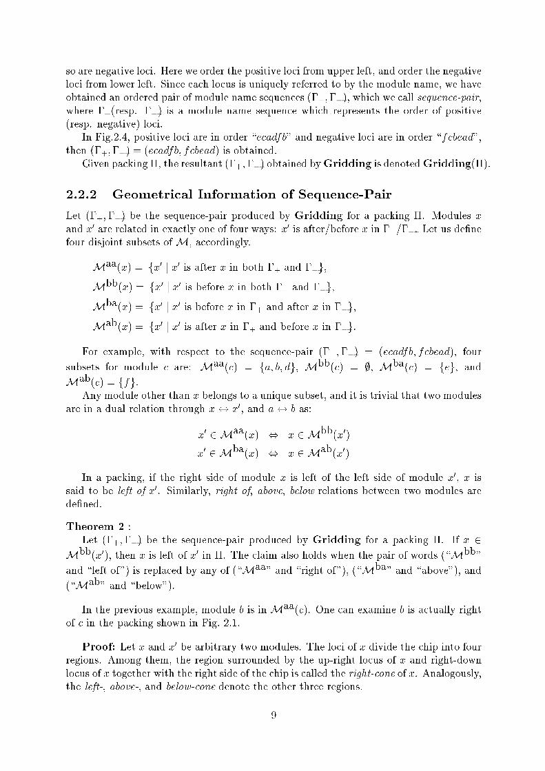
2.2.2 Geometrical Information of Sequence-Pair

Let (�+;��) be the sequence-pair produced by Gridding for a packing �. Modules x

and x0 are related in exactly one of four ways: x0 is after/before x in �+=��. Let us de�ne

four disjoint subsets ofM, accordingly.

Maa(x) = fx0 j x0 is after x in both �+ and ��g,

Mbb(x) = fx0 j x0 is before x in both �+ and ��g,

Mba(x) = fx0 j x0 is before x in �+ and after x in ��g,

Mab(x) = fx0 j x0 is after x in �+ and before x in ��g.

For example, with respect to the sequence-pair (�+;��) = (ecadfb; fcbead), four

subsets for module c are: Maa(c) = fa; b; dg, Mbb

(c) = ;, Mba(c) = feg, and

Mab(c) = ffg.

Any module other than x belongs to a unique subset, and it is trivial that two modules

are in a dual relation through x$ x0, and a$ b as:

x0 2Maa(x) , x 2 Mbb

(x0)

x0 2Mba(x) , x 2 Mab

(x0)

In a packing, if the right side of module x is left of the left side of module x0, x is

said to be left of x0. Similarly, right of, above, below relations between two modules are

de�ned.

Theorem 2 :

Let (�+;��) be the sequence-pair produced by Gridding for a packing �. If x 2Mbb

(x0), then x is left of x0 in �. The claim also holds when the pair of words (\Mbb"

and \left of") is replaced by any of (\Maa" and \right of"), (\Mba

" and \above"), and

(\Mab" and \below").

In the previous example, module b is inMaa(c). One can examine b is actually right

of c in the packing shown in Fig. 2.1.

Proof: Let x and x0 be arbitrary two modules. The loci of x divide the chip into four

regions. Among them, the region surrounded by the up-right locus of x and right-down

locus of x together with the right side of the chip is called the right-cone of x. Analogously,

the left-, above-, and below-cone denote the other three regions.

9

Suppose x0 is inMaa(x). This implies that the positive locus of x0 is in the union of

the right-cone and the below-cone of x. Also it is implied that the negative locus of x0 is

in the union of the right-cone and the above-cone of x. The cross point of the positive

locus and the negative locus of x0 is in their intersection, that is, the right-cone of x.

Then, module x0 is in the right-cone of x. Every modules in the right-cone of x is right

of module x by de�nition of the up-right locus and the right-down locus of x.

It is clear that the claim holds for the other cases. 2

2.3 From Sequence-Pair to Packing

In the previous section, we analyzed the packing and �xed the procedure Gridding to

obtain one sequence-pair from a given packing. Now we provide a procedure to synthesize

one packing from an arbitrary sequence-pair.

2.3.1 Constraint of Sequence-Pair

Given a sequence-pair (�+;��), we read a constraint from it as follows.

The Constraint Implied by a Sequence-Pair (�+;��)

If x 2 Mbb(x0), module x must be left of module x0. This is also the constraint with

replacing the pair of words (\Mbb" and \left of") with any of (\Maa

" and \right of"),

(\Mba" and \above"), and (\Mab

" and \below").

It is easily seen that the constraint imposed on the packing by a sequence-pair is

unique. Furthermore, the following theorem holds.

Theorem 3 : The constraint is always satis�able.

Proof: Consider an n� n grid. Label the horizontal grid lines and vertical grid lines

with module names along �+ and �� from top and from left, respectively. A cross point

of the horizontal grid line of label x and the vertical grid line of label x0 is referred to

by (x; x0). Then, rotate the resultant grid by 45 degrees counter clockwise to get an

oblique grid. (See Fig. 2.6.) Put each module x with its center being on (x; x). Expand

the separation of grid lines

p2 times larger than the longest width/height over modules,

which is su�cient to eliminate overlapping of modules. The resultant packing trivially

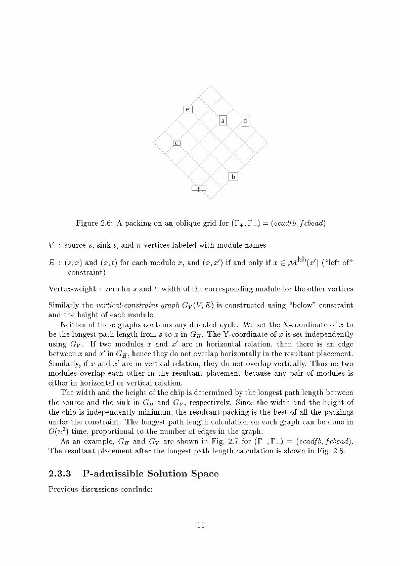
satis�es the constraint implied by the given sequence-pair. 2

An example is shown in Fig. 2.6.

2.3.2 Best Packing Under the Constraint

Given (�+;��), one of the optimal packings under the constraint can be obtained in

O(n2) time by applying the well-known longest path algorithm for vertex weighted directed

acyclic graphs. The process is given below.

Based on \left of" constraint of (�+;��), a directed and vertex-weighted graphGH(V;E)

(V : vertex set, E: edge set), called the horizontal-constraint graph, is constructed as fol-

lows.

10

e

c

a d

b

f

Figure 2.6: A packing on an oblique grid for (�+;��) = (ecadfb; fcbead)

V : source s, sink t, and n vertices labeled with module names

E : (s; x) and (x; t) for each module x, and (x; x0) if and only if x 2 Mbb(x0) (\left of"

constraint)

Vertex-weight : zero for s and t, width of the corresponding module for the other vertices

Similarly the vertical-constraint graph GV (V; E) is constructed using \below" constraint

and the height of each module.

Neither of these graphs contains any directed cycle. We set the X-coordinate of x to

be the longest path length from s to x in GH . The Y-coordinate of x is set independently

using GV . If two modules x and x0 are in horizontal relation, then there is an edge

between x and x0 in GH , hence they do not overlap horizontally in the resultant placement.

Similarly, if x and x0 are in vertical relation, they do not overlap vertically. Thus no two

modules overlap each other in the resultant placement because any pair of modules is

either in horizontal or vertical relation.

The width and the height of the chip is determined by the longest path length between

the source and the sink in GH and GV , respectively. Since the width and the height of

the chip is independently minimum, the resultant packing is the best of all the packings

under the constraint. The longest path length calculation on each graph can be done in

O(n2) time, proportional to the number of edges in the graph.

As an example, GH and GV are shown in Fig. 2.7 for (�+;��) = (ecadfb; fcbead).

The resultant placement after the longest path length calculation is shown in Fig. 2.8.

2.3.3 P-admissible Solution Space

Previous discussions conclude:

11

e

c

a d

b

f

e

c

a d

b

f

Figure 2.7: Constraint graphs GH(left) and GV (right) (transitive edges are not drawn for

simplicity)

e

c

f

a d

b

Figure 2.8: A best packing under the constraint implied by (�+;��) = (ecadfb; fcbead)

12

Theorem 4 : The set of all sequence-pairs is a P-admissible solution space of RP. More

precisely, it consists of (n!)2 sequence-pairs, each of which can be mapped to a packing in

O(n2) time, and at least one of which corresponds to one of the optimal solutions of RP.

2

Our discussion started for minimizing the area of the chip. However, all the discussions

hold as long as the evaluating function is independently non-decreasing with respect to

the width and the height of the chip. Therefore we may assume instead, for example,

perimeter of the chip, area of the chip of pre-speci�ed aspect ratio, and the height of the

chip when its width is �xed. This fact will extend the usefulness of our solution space.

It has also been assumed that the orientation of each module (vertically laid or hori-

zontally laid) is �xed. When the orientation is also requested to be optimized, we hold a

f0; 1g sequence of length n, expressing the orientation of each module being horizontal or

vertical. The size of solution space increases to (n!)22m. (The orientation optimization for

a �xed rectangular dissection is known to be NP-hard [17].) This technique can be easily

extended to so-called \soft" modules, by preparing three or more candidates of (width,

height) per module [18].

There is a sequence-pair for which another sequence-pair provides no worse packing,

independent of the sizes of the modules. For example, if (abcd; cdab) corresponds to an

optimal packing, then (abcd; cadb) or (acbd; cdab) also corresponds to an optimal packing,

regardless of the widths and the heights of modules a; b; c and d. Then, the former

sequence-pair, (abcd; cdab), is redundant for our current objective to �nd a packing with

smaller area. We extend our evaluating function to consider wires in the next section.

2.4 Use of Sequence-Pair

2.4.1 Rectangle Packing

We use a standard simulated annealing method to pack rectangles. It uses two kinds of

pair-interchanges: (i) two module names in �+, (ii) two module names in �+ and also

in ��. The initial sequence-pair was made at random. The temperature was decreased

exponentially.

The �rst interest would be to know the experimental performance ratio (obtained

area / optimal area) of the above described simulated annealing. For this purpose, two

problem instances are constructed such that their optimal solutions are known.

REGGRID : a collection of 100 unit squares. It is easily understood that an optimal

solution with area 100 is possible when the squares are packed in the 10�10 regulargrid.

LOGGRID : a collection of 100 rectangles, generated by an exponential grid formed

by eleven vertical lines x = 0; 1; 2; 3; 5; 7; 10; 14; 19; 26; 36 and eleven horizontal lines

y = 0; 1; 2; 3; 5; 7; 10; 14; 19; 26; 36. Thus, the area of the optimal solution is 36�36 =1296.

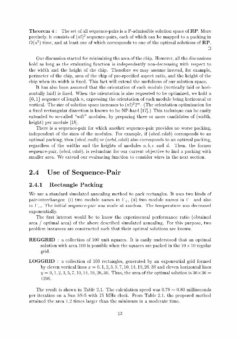
The result is shown in Table 2.1. The calculation speed was 0:78 � 0:80 milliseconds

per iteration on a Sun SS-5 with 75 MHz clock. From Table 2.1, the proposed method

attained the area 1:2 times larger than the minimum in a moderate time.

13

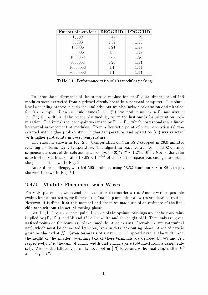
Number of iterations REGGRID LOGGRID

10000 1:44 1:29

30000 1:32 1:33

100000 1:21 1:17

300000 1:3 1:17

1000000 1:08 1:20

3000000 1:20 1:14

10000000 1:1 1:11

30000000 1:1 1:14

Table 2.1: Performance ratio of 100 modules packing

To know the performance of the proposed method for \real" data, dimensions of 146

modules were extracted from a printed circuit board in a personal computer. The simu-

lated annealing process is designed similarly, but we also include orientation optimization

for this example: (i) two module names in �+, (ii) two module names in �+ and also in

��, (iii) the width and the height of a module, where the last one is for orientation opti-

mization. The initial sequence-pair was made as �+ = ��, which corresponds to a linear

horizontal arrangement of modules. From a heuristic point of view, operation (i) was

selected with higher probability in higher temperature, and operation (iii) was selected

with higher probability in lower temperature.

The result is shown in Fig. 2.9. Computation on Sun SS-2 stopped in 29.9 minutes

reaching the terminating temperature. The algorithm searched at most 606,192 distinct

sequence-pairs out of the solution space of size (146!)22146 � 1:23�10552. Notice that, the

search of only a fraction about 4:92� 10�547

of the solution space was enough to obtain

the placement shown in Fig. 2.9.

As another challenge, we tried 500 modules, using 18.83 hours on a Sun SS-2 to get

the result shown in Fig. 2.10.

2.4.2 Module Placement with Wires

For VLSI placement, we extend the evaluation to consider wires. Among various possible

evaluations about wires, we focus on the �nal chip area after all wires are detailed-routed.

However, it is di�cult at this moment and hence we made use of an estimate of the �nal

chip area without the actual routing phase.

Let (�+;��) be a sequence-pair, � be one of the optimal packings under the constraint

implied by (�+;��), andW and H be the width and the height of �. Terminals are given

as �xed points on the boundary of each module. A net is a set of terminals (multi-terminal

net), which must be connected by wires, later in detailed-routing phase. A set of nets is

given as the netlist N . Given terminals of a net i, which spread over �, the width and

the height of the smallest bounding box of these terminals are denoted by Wi and Hi,

respectively. T is the sum of wiring width and wiring space (obtained from a design rule

set). We use the following formula proposed in [13] to estimate the �nal chip width W 0

and height H 0.

14

Figure 2.9: Packing of 146 modules

Figure 2.10: Packing of 500 modules

15

W 0= W + T

�i2NHi

H

H 0= H + T

�i2NWi

W

The second term of each formula estimates the increase in one direction owing to the

wires, assuming all wires are uniformly distributed in the �nal chip. They experimentally

showed that the result is acceptable for a commercial channel router [13].

There are choices per module, which is the combination of the four choices of 0; 90; 180; 270

degree rotations, and a decision yes, no on re ecting the module about the Y axis. This

code for orientation and a sequence-pair are put together into a simulated annealing

process in our system. The process runs in a similar fashion as the rectangle packing

optimization, and explores the solution space of size (n!)28n.

A point not mentioned in [13] is how the location of each individual module is cal-

culated. In our system, after the best evaluated code is obtained, coordinates of each

module are determined as follows. Assume (Xj; Yj) is the coordinates of the lower left

corner of module j in �. (This is the information we can use in this phase.) Let NXj be

a set of nets such that the X coordinate of the left side of bounding box of the net is less

than or equal to Xj. Similarly, NYj is de�ned using Yj . We determine the coordinates

(X 0j ; Y

0j ) of the lower left corner of module j in the resultant chip by the following formula.

X 0j = Xj + T

�i2NXj

Hi

H

Y 0j = Yj + T

�i2NYj

Wj

W

For an experiment, the biggest building block layout data, called \ami49", was taken

from the MCNC benchmarks. The data is the biggest one in their benchmark suit, but our

method was fast enough to handle the data without splitting the problem. (Some recent

research [9] also handle the data without dividing the problem.) The result is shown in

Fig. 2.11. We remark that it was done with an additional constraint: aspect ratio = 1,

taking T = 7 �m. The estimated chip size is 6482 �m � 6925 �m. Computation time

was 31:36 minutes on SunIPX.

2.5 Conclusion

This chapter introduced a data structure to represent a general packing in terms of a pair

of module name sequences, called sequence-pair. Detailed proofs are presented to show

that every sequence-pair feasibly corresponds to a packing, and at least one sequence-pair

corresponds to an area-minimum packing.

In experiments, 500 rectangles were packed very e�ciently in a reasonable time. It was

attained by a standard simulated annealing in which a move is a change of the sequence-

pair. The evaluating function was then extended to the VLSI placement problem using

a conventional wiring area estimation method. The biggest MCNC benchmark, ami49, is

placed very nicely.

16

Figure 2.11: Placement of MCNC \ami49"

17

Chapter 3

Mapping from Sequence-Pair to

Rectangular-Dissection

3.1 Introduction

In the �rst stage of VLSI physical design, it is required to determine a rough arrangement

of circuit components, such as modules and channels. A stochastic algorithm, such as

simulated annealing or genetic algorithm, would be a good choice as an optimization

algorithm since the problem is hard. To make a stochastic algorithm work e�ectively, a

fundamental issue is in how to represent candidate arrangements, with enough generality

and e�ciency to cope with various design requirements.

In Chapter 2, we proposed a representation called sequence-pair , which is a pair of

module name sequences. For example, (abc; cab) is a sequence-pair for module set fa; b; cg.For a sequence-pair, they assigned an HV-relation-set (HVRS), which is a set of horizontal

(right of/left of) or vertical (above/below) relations for every module pair. For example,

sequence-pair (abc; cab) corresponds to HVRS fa is left of b, c is below a, c is below

bg. It is proved in the chapter that a sequence-pair always corresponds to a realizable

HVRS, and there is a sequence-pair whose HVRS can lead an area minimum placement.

However, HVRS alone is not su�cient as a representation of candidate arrangements of

components. Channel positions are also desired to be represented together.

A traditional method exists to represent channel positions together with module posi-

tions. It is the rectangular-dissection. (sometimes called oorplan in the literature [17].)

However, known e�cient representation techniques are limited for speci�c classes of

rectangular-dissections, such as slicing structure [8].

To combine the merits of sequence-pair and rectangular-dissection, it is desired to map

a sequence-pair to a rectangular-dissection. Observe from Fig. 3.2-(a) that a room with

no module assignment, called the empty room, is necessary in the rectangular-dissection

to keep the relative positions of modules. It is worth allowing this empty room since

it is essentially needed to achieve the area minimum placement. However, introducing

arbitrary many empty rooms results in arbitrary many line segments, which represent

channels.

This chapter gives a mapping from a sequence-pair to a rectangular-dissection whose

number of rooms is minimum among all the rectangular-dissections whose HVRSs are

equivalent to the HVRS of the given sequence-pair. Consequently, candidate arrangements

of modules and channels are successfully represented with the generality and the e�ciency

18

inherited from the sequence-pair.

The organization of this chapter is as follows. Section 3.2 de�nes preliminary terms.

Section 3.3 shows a necessary and su�cient condition that a sequence-pair is mapped to

a rectangular-dissection with no empty room. Section 3.4 presents a procedure to output

a rectangular-dissection with fewest empty rooms. Section 3.5 is for conclusion.

3.2 Preliminary

3.2.1 HV-Relation-Set

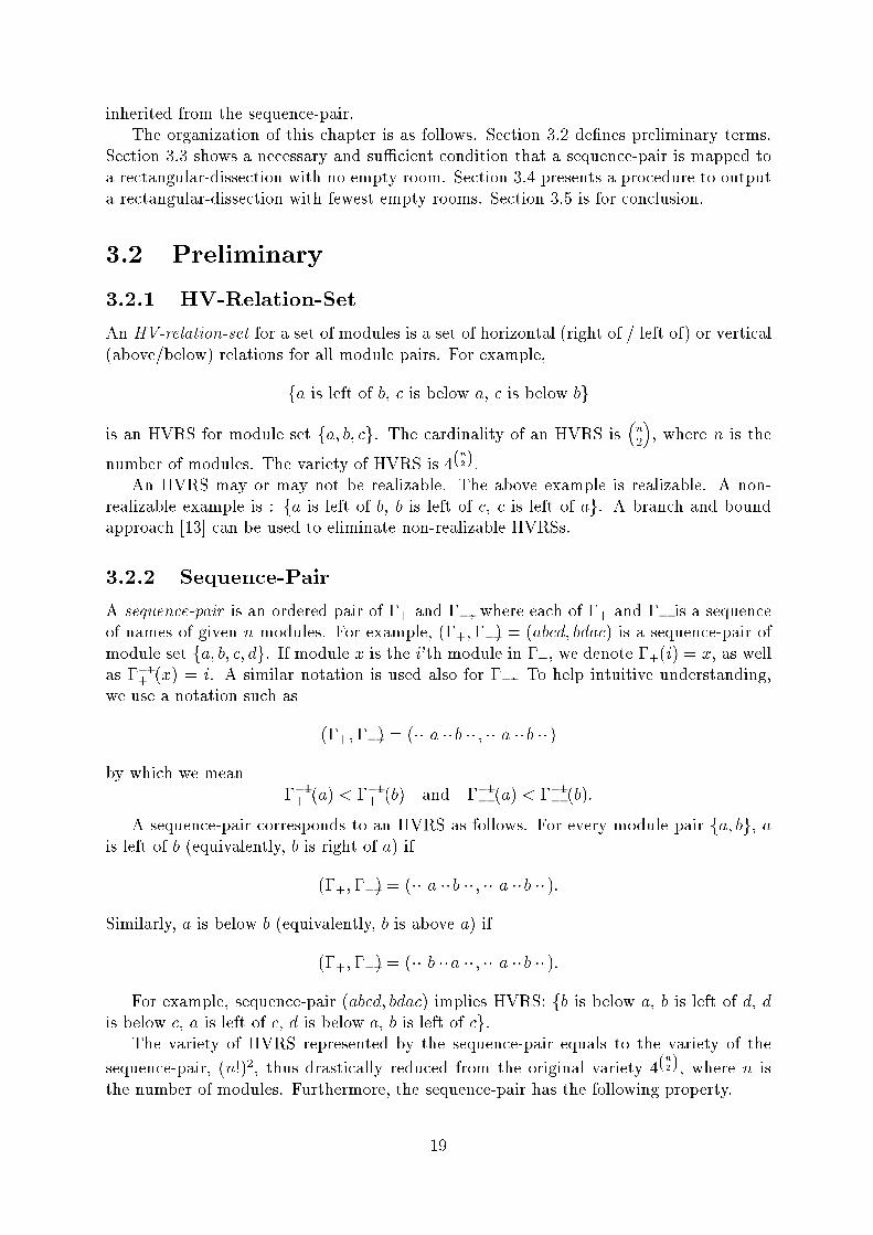
An HV-relation-set for a set of modules is a set of horizontal (right of / left of) or vertical

(above/below) relations for all module pairs. For example,

fa is left of b, c is below a, c is below bg

is an HVRS for module set fa; b; cg. The cardinality of an HVRS is

�n

2

�, where n is the

number of modules. The variety of HVRS is 4(n

2).

An HVRS may or may not be realizable. The above example is realizable. A non-

realizable example is : fa is left of b, b is left of c, c is left of ag. A branch and bound

approach [13] can be used to eliminate non-realizable HVRSs.

3.2.2 Sequence-Pair

A sequence-pair is an ordered pair of �+ and ��, where each of �+ and �� is a sequence

of names of given n modules. For example, (�+;��) = (abcd; bdac) is a sequence-pair of

module set fa; b; c; dg. If module x is the i'th module in �+, we denote �+(i) = x, as well

as ��1+(x) = i. A similar notation is used also for ��. To help intuitive understanding,

we use a notation such as

(�+;��) = (�� a ��b �� ; �� a ��b ��)

by which we mean

��1+(a) < �

�1+(b) and �

�1� (a) < �

�1� (b):

A sequence-pair corresponds to an HVRS as follows. For every module pair fa; bg, ais left of b (equivalently, b is right of a) if

(�+;��) = (�� a ��b �� ; �� a ��b ��):

Similarly, a is below b (equivalently, b is above a) if

(�+;��) = (�� b ��a �� ; �� a ��b ��):

For example, sequence-pair (abcd; bdac) implies HVRS: fb is below a, b is left of d, d

is below c, a is left of c, d is below a, b is left of cg.The variety of HVRS represented by the sequence-pair equals to the variety of the

sequence-pair, (n!)2, thus drastically reduced from the original variety 4(n

2), where n is

the number of modules. Furthermore, the sequence-pair has the following property.

19

a

b

c

d

a

b

c

d

(a) (b)

Figure 3.1: (a) Sequence-Pair (abcd; bdac), (b) Horizontal-Seq-Pair-Graph (H-SPG) and

Vertical-Seq-Pair-Graph (V-SPG). The edges of H-SPG are drawn in solid lines and the

edges of V-SPG are drawn in dotted lines.

Property 1 : The HVRS of every sequence-pair is realizable. For any non-overlapping

placement, there is a sequence-pair whose HVRS is satis�ed by the placement. 2

A proof is given in Chapter 2.

The HVRS of a sequence-pair of n modules can be graphically understood by means

of oblique-grid , de�ned as follows. Let L+(1); L+(2); � � � ; L+(n) be n parallel lines of slope

+1 drawn on a plane, ordered from left. Let L�(1); L�(2); � � � ; L�(n) be n parallel lines

of slope �1 drawn on the plane, also ordered from left. These 2n lines form a 45 degree

oblique n � n grid, called the oblique-gird . The oblique-grid-embedding of a sequence-

pair (�+;��) is the oblique-grid with each module name x written at the cross point of

L+(��1+(x)) and L�(�

�1� (x)). Fig. 3.1-(a) shows the oblique-grid-embedding of sequence-

pair (abcd; bdac). Using the oblique-grid-embedding, the HVRS of a sequence-pair can be

re-de�ned as: for each module x, the modules which are seen from x in the angle between

�45 degree and 45 degree are right of x, the modules in the angle between 45 degree and

135 degree are above x, and so on.

The HVRS of a sequence-pair is represented by a pair of directed acyclic graphs,

called horizontal-sequence-pair-graph (H-SPG) and vertical-sequence-pair-graph (V-SPG),

de�ned as follows. For either graph, vertices uniquely correspond to modules and have

the corresponding module names. The edge set of the H-SPG is constructed faithfully to

the horizontal relations, from left to right, but eliminating the transitive edges. The edge

set of the V-SPG is de�ned similarly from bottom to top. We sometime abbreviate the

pair of H-SPG and V-SPG of a sequence-pair to \SPGs".

Oblique-grid-embedding of a sequence-pair with arrows additionally drawn corre-

sponding to the edges of the SPGs is called the oblique-grid-embedding of the SPGs.

Fig. 3.1-(b) shows an example, where the edges of the H-SPG are drawn using solid lines,

and the edges of the V-SPG are drawn using dotted lines.

20

3.2.3 Rectangular-Dissection

A rectangular-dissection is a dissection of a rectangle into a set of rectangles, called rooms,

with an injective assignment of modules to rooms (no two modules share a room.) An

example is shown in Fig. 3.2-(a). Only T-intersections are used to form the dissection

except for the four corners of the bounding rectangle. (Two T-intersections may form a

cross shape as a degenerate case.) The bounding rectangle represents the chip, each room

represents an area which is assignable to a module, and each line segment represents a

channel. A room is said to be occupied if a module is assigned to the room, otherwise

said to be empty. In Fig. 3.2-(a), the dark room at the center is empty and the other

rooms are occupied. Empty rooms have been used to modify a rectangular-dissection

incrementally [19].

A rectangular-dissection speci�es relative positions of modules and channels as follows:

If the right side of a room ra and the left side of a room rb are both on an identical vertical

line segment lc, the module a assigned to the room ra should be placed left of the channel

c corresponding to the line segment lc, and the module b assigned to the room rb should

be placed right of the channel c (horizontal relation). Notice that a horizontal relation

between module pair a; b is transitively speci�ed as: module a should be placed left of

module b. Vertical relations are speci�ed similarly using horizontal line segments.

The information of a rectangular-dissection is commonly represented by means of a

pair of directed acyclic graphs [20, 21, 17], a horizontal-rectangular-dissection-graph (H-

RDG) and a vertical-rectangular-dissection-graph (V-RDG). Each vertical (horizontal)

line segment corresponds to a vertex in the H-RDG (V-RDG) and each room corresponds

to an edge (u; v) where u is the vertex corresponding to the left (bottom) side of the room

and v is the vertex corresponding to the right (top) side of the room. We sometime use the

word \RDGs" to denote the pair of H-RDG and V-RDG of a rectangular-dissection. Two

rectangular-dissections are said to be equivalent if their RDGs (the two H-RDGs, as well

as the two V-RDGs) are the same. Fig. 3.2-(b) illustrates the RDGs of the rectangular-

dissection shown in Fig. 3.2-(a). In the �gure, the edges of H-RDG are drawn using solid

lines, and the edges of V-RDG are drawn using dotted lines. An empty room corresponds

to the anonymous edge in the �gure.

H-RDG as well as V-RDG is a directed acyclic planar graph with possibly duplicated

edges. Each RDG is polar, i.e. a directed acyclic graph with a single source and a single

sink. Two polar graphs G1 and G2 are said to be in polar-dual relation if G1 and G2

become dual when an undirected edge from the source to the sink is added in each graph.

From the construction, the RDGs are in polar-dual relation. The reverse is also true since

polar-dual graphs are known to be mapped to a rectangular-dissection [21].

Property 2 : Given two polar graphs G1 and G2, there exists a rectangular-dissection

whose RDGs are G1 and G2, if and only if G1 and G2 are in polar-dual relation. 2

When we construct a rectangular-dissection from H-RDG Gh and V-RDG Gv, we use

the following procedure.

Procedure ConstRD(Gh; Gv)

For a vertex u 2 V (Gh), x(u) denotes the ordinal number of the vertex u in a topological

order of the vertices in Gh. (x(u) has a unique integer such that x(u) < x(u0) if there

exists a path from u to u0). Similarly, y(v) denotes the ordinal number of the vertex v

21

a

b

c

d

ac

b

d

(a) (b)

Figure 3.2: (a) Rectangular-Dissection, (b) Horizontal-Rectangular-Dissection-Graph (H-

RDG) and Vertical-Rectangular-Dissection-Graph (V-RDG). H-RDG is drawn in solid

lines and V-RDG is drawn in dotted lines.

in a topological order of the vertices in Gv. A pair of edges (eh; ev) is called a \cross" if

eh(2 E(Gh)) and ev(2 E(Gv)) are in a dual relation. For each cross ((u1; u2); (v1; v2)),

draw a rectangle whose lower left corner is at (x(u1); y(v1)) and whose upper right corner

is at (x(u2); y(v2)). (Procedure ConstRD End)

It is easily seen that ConstRD runs in O(n) time, where n = jE(Gh)j = jE(Gv)j whichalso equals to the number of rooms in the resultant rectangular-dissection.

3.2.4 Sequence-Pair and Rectangular-Dissection

The major merit of the sequence-pair and that of the rectangular-dissection are summa-

rized as follows.

� The merit of the sequence-pair is in its e�ciency in enumerating various HVRSs.

� The merit of the rectangular-dissection is in its ability of representing the channels.

To keep the two merits at the same time, the target of this chapter is:

Target: To map a sequence-pair to a rectangular-dissection.

The following three properties show a similarity of the sequence-pair and the rectangular-

dissection.

Property 3 : Given a sequence-pair, for any two modules a and b, there is a path which

connects a and b in H-SPG or in V-SPG, but not in both. 2

Property 4 : In the H-RDG (V-RDG) of a rectangular-dissection, if there is a path from

edge a to edge b, then the room a is left of (below) room b in the rectangular-dissection.

2

Property 3 and 4 are easily understood.

22

Property 5 : Given a rectangular-dissection, for any two rooms a; b, there is a path

which connects a and b in H-RDG or in V-RDG, and not in both.

Proof : Let G and G0be the H-RDG and V-RDG of the rectangular-dissection. Then

G and G0are in polar-dual relation. Let source and sink of G(G0

) be s(s0) and t(t0),

respectively. A full-path of G(G0) is a path from s(s0) to t(t0) in G(G0

). Then the claim

can be re-written as: for any two edges a and b, a full-path which includes both a and b

exists either in G or G0, and not exists in both G and G0

.

It is clear that G and G0are in polar-dual relation. Hence, the edge set of a full-path

of G(G0) has one to one correspondence with a cut set of G0

(G).

If G has a full-path which includes both a and b, there is a cut set in G0which includes

both a and b, hence G0does not have a full-path which includes both a and b.

In the following, we consider the case G does not have a full-path which includes both

a and b. Let VR be the subset of vertices in G consists of the vertices which is reachable

from the outgoing vertex of a or the outgoing vertex of b. Let VR be the rest. Since G is a

directed acyclic graph, the incoming vertex of G and the incoming vertex of G0are both

in VR. There is no edge from a vertex in VR to a vertex in VR, hence the set of edges from

a vertex in VR to a vertex in VR is a cut, and the cut includes both a and b. Therefore,

G0has a full-path which includes both a and b. 2

Property 4 and 5 imply that a rectangular-dissection, as well as a sequence-pair,

uniquely corresponds to an HVRS. Then, the correspondence between the sequence-pair

and the rectangular-dissection is in question. Next property can be easily derived from

the result of Chapter 2.

Property 6 : For the HVRS T of any rectangular-dissection, there is unique sequence-

pair S whose HVRS is T . 2

The reverse direction is essential to achieve our target. We have the following obser-

vations.

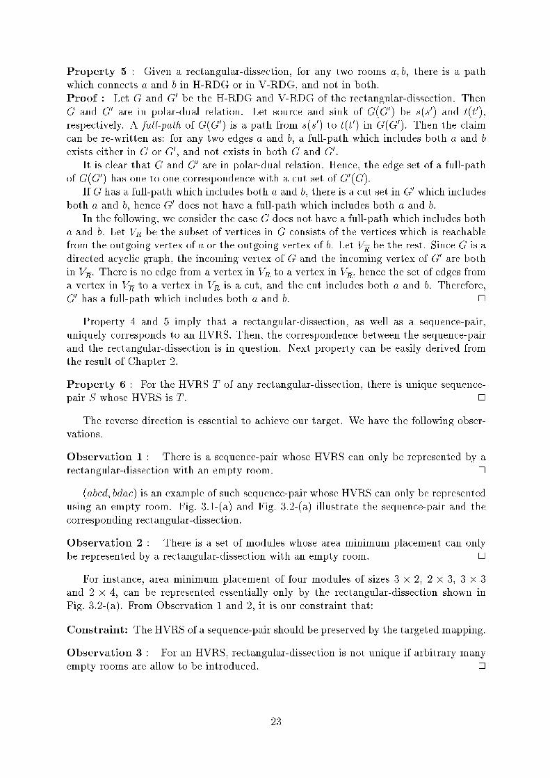
Observation 1 : There is a sequence-pair whose HVRS can only be represented by a

rectangular-dissection with an empty room. 2

(abcd; bdac) is an example of such sequence-pair whose HVRS can only be represented

using an empty room. Fig. 3.1-(a) and Fig. 3.2-(a) illustrate the sequence-pair and the

corresponding rectangular-dissection.

Observation 2 : There is a set of modules whose area minimum placement can only

be represented by a rectangular-dissection with an empty room. 2

For instance, area minimum placement of four modules of sizes 3 � 2, 2 � 3, 3 � 3

and 2 � 4, can be represented essentially only by the rectangular-dissection shown in

Fig. 3.2-(a). From Observation 1 and 2, it is our constraint that:

Constraint: The HVRS of a sequence-pair should be preserved by the targeted mapping.

Observation 3 : For an HVRS, rectangular-dissection is not unique if arbitrary many

empty rooms are allow to be introduced. 2

23

Property 7 : For any rectangular-dissection, the number of line segments is equal to

the number of rooms plus three. 2

Property 7 can be proved by counting the number of room corners contributed by a

line segment.

Recall that the line segments represent channels. Although the goodness about the

number of channels might di�er in several routing schemes, fewer number of channels is

most likely preferred to avoid too many wire bends. Thus, it is our criterion that:

Criterion: Minimize the number of rooms in the targeted mapping.

3.3 Rectangular-Dissection without Empty Room

This section gives a procedure which maps a sequence-pair to a rectangular-dissection

without any empty room if the given sequence-pair satis�es a certain condition. Then,

the condition is revealed to be necessary and su�cient for eliminating the introduction

of empty room. To describe the condition, we need to de�ne two terms, HV-cross and

adjacent-cross.

3.3.1 HV-Cross and Adjacent-Cross

Four modules a; b; c; d are said to form an HV-cross in a sequence-pair S = (�+;��) if

they satisfy the following three conditions in (�+;��) or in (�+;�0�), where �

0� is the

reverse of ��.

� (�� a ��b ��c ��d �� ; �� c ��a ��d ��b ��)� There is no module x which satis�es

(�� a ��x ��d �� ; �� a ��x ��d ��):

� There is no module x which satis�es

(�� b ��x ��c �� ; �� c ��x ��b ��):

Fig. 3.3-(a) illustrates an HV-cross using oblique-grid. There is no module in the dark

region because of the last two conditions in the de�nition. HV-cross is so called because

it corresponds to a crossing between an edge in the H-SPG and an edge in the V-SPG in

the oblique-grid-embedding of the SPGs.

If four modules a; b; c; d form an HV-cross and b and c are adjacent in �+, and a and

d are adjacent in ��(�0�), the HV-cross is also called the adjacent-cross. The condition

is illustrated in Fig. 3.3-(b).

Lemma 1 : If there is an HV-cross in a sequence-pair S, then an adjacent-cross also

exists in S.

Proof : The proof is by contradiction. Without loss of generality, let an HV-cross formed

by four modules a; b; c and d be S = (�+;��) = (�� a ��b ��c ��d �� ; �� c ��a ��d ��b ��). (See

24

a

b

c

d

ab

cd

adjacentadjacent

(a) (b)

Figure 3.3: (a) HV-cross (no module is in the dark region). (b) adjacent-cross (special

case of HV-cross).

Fig. 3.4.) We can assume further that: (i) the distance between b and c in �+ is minimal

over all the HV-crosses in S; and (ii) among such HV-crosses, the distance between a and

d in �� is minimal.

If b and c are not adjacent in �+, there is a module in between. Such modules are not

between b and c in ��, from the de�nition of HV-cross. In such modules, there is module

x which satis�es one of the two cases:

� S = (�� a ��b ��x ��c ��d �� ; �� x ��c ��a ��d ��b ��) and a; b; x; d form an HV-cross, or

� S = (�� a ��b ��x ��c ��d �� ; �� c ��a ��d ��b ��x ��) and a; x; c; d form an HV-cross.

(Fig. 3.4 illustrates an example for the former case.) Either case contradicts to the

assumption (i). Similarly, if a and d are not adjacent in ��, a contradiction to the

assumption (ii) is derived. Hence, a; b; c; d form an adjacent-cross. 2

3.3.2 Converting Sequence-Pair into Rectangular-Dissection

A procedure called SeqPair{RDG is presented to map a sequence-pair to a pair of RDGs.

From the resultant RDGs, a rectangular-dissection is obtained by the procedure ConstRD

given in Section 3.2. Fig. 3.5 illustrates the result of each step for input sequence-pair

S = (abcde; becad). A hyper directed edge is denoted (Vi; Vo), where Vi is the input vertex

set, and Vo is the output vertex set.

Procedure SeqPair{RDG

Input: Sequence-pair S = (�+;��) which has no adjacent-cross.

Output: H-RDG GHP and V-RDG GV P .

(Step 1) Add four new modules sh; th; sv; tv, called phantom modules, to the input

sequence-pair S = (�+;��) and obtain new sequence-pair S? = (tvsh�+thsv; svsh��thtv).

Construct H-SPG GHSP and V-SPG GV SP from S?.

25

a

b

c

dx

Figure 3.4: Figure used in the proof of Lemma 1

(Step 2) Construct a horizontal hyper graph GH and a vertical hyper graph GV from

GHSP and GV SP as follows. The vertex set of GH and GV are both equivalent to the

vertex set of SPGs. A hyper edge (VL; VR) is in the edge set E(GH) if and only if the

subgraph of GHSP induced by VL [ VR is a maximal bipartite. The edge set E(GV ) is

similarly de�ned using GV SP .

(Step 3) For GH (also for GV ), construct a hyper graph GHP (resp. GV P ) by converting

all the hyper edges to the vertices and by converting all the vertices, except for the vertices

corresponding to the phantom modules, to the edges. (Procedure SeqPair{RDG End)

Theorem 5 : Let S be a sequence-pair of nmodules. If S does not include adjacent-cross,

procedure SeqPair{RDG maps S to a pair of RDGs which correspond to a rectangular-

dissection with no empty room such that the HVRS of the rectangular-dissection equals

to the HVRS of S, in O(n2) time. 2

From the resultant RDGs, a rectangular-dissection is obtained by ConstRD in O(n)

time. In the following, we prove this theorem.

Lemma 2 : In (Step 1), each edge of GHSP (GV SP ) belongs to a unique maximal

complete bipartite subgraph of GHSP (GV SP ).

Proof : The proof is by contradiction. Assume an edge (a1; b1) belongs to two maximal

complete bipartite subgraphs G1(V 1

i [ V 1

o ; E1) and G2

(V 2

i [ V 2

o ; E2). Since G1

and G2

are both maximal complete bipartite graphs, there are two vertices a2 2 (V 1

i [ V 2

i ) and

b2 2 (V 1

o [ V 2

o ) such that there is no edge (a2; b2) in E(GHSP ). The edges (a1; b1), (a1; b2)

and (a2; b1) all exist in E(GHSP ). If a1 and a2 are in horizontal relation, then (a1; b1)

or (a2; b1) becomes transitive. Hence a1 and a2 are in vertical relation. Without loss of

generality, we assume a1 is above a2, i.e. S = (�� a1 ��a2 �� ; �� a2 ��a1 ��). Since there areedges (a1; b1) and (a2; b1), S = (�� a1 ��a2 ��b1 �� ; �� a2 ��a1 ��b1 ��). Considering the fact thatthere is edge (a1; b2), the position of b2 are exhaustively examined in the following. (See

Fig. 3.6).

(i) S = (�� a1 ��b2 ��a2 ��b1 �� ; �� a2 ��a1 ��b1 ��b2 ��)

26

t v

t hsh

s v

c

d

e

a

b

(a) GHSP (solid lines) and GV SP (dotted lines) obtained in Step 1

t v

t hsh

s v

c

d

e

a

b

(b) GH (solid lines) and GV (dotted lines) obtained in Step 2

a

bc

e

d

(c) GHP (solid lines) and GV P (dotted lines) obtained in Step 3

Figure 3.5: Snapshot of the procedure SeqPair{RDG

27

a 1

a 2

b1

b2

b2

b 2

(i)

(ii)

(iii)

Figure 3.6: Figure used in the proof of Lemma 2

In GV SP , there is a path from a2 to b2. An edge in the path crosses to the edge

(a1; b1) 2 E(GHSP ), thus there is an HV-cross in S. This contradicts to the fact

that S has no adjacent-cross (thus no HV-cross by Lemma 1).

(ii) S = (�� a1 ��a2 ��b2 ��b1; �� a2 ��a1 ��b1 ��b2 ��)Since edge (a2; b2) does not exist in E(GHSP ), there is a vertex x which satis�es

S = (��a1 ��a2 ��x��b2 ��b1; ��a2 ��x��a1 ��b1 ��b2) or S = (��a1 ��a2 ��x��b2 ��b1; ��a2 ��a1 ��b1 ��x��b2).The former case results in (a2; b1) being transitive, and the latter results in (a1; b2)

being transitive, either contradicts to the de�nition of GHSP .

(iii) S = (�� a1 ��a2 ��b1 ��b2 �� ; �� a2 ��a1 ��b2 ��b1 ��)Since there is no edge (a2; b2), there is module x which satis�es S = (�� b1 ��x ��b2 �� ; �� a2 ��x ��a1). Then, there is a path from x to a1 in GV SP . An edge in the path

crosses to the edge (a2; b1) 2 E(GHSP ), which is a contradiction.

(iv) The other cases are trivially impossible.

Hence, an edge in GHSP belongs to a unique maximal bipartite subgraph of GHSP . Sim-

ilarly, the claim also holds for GV SP . 2

Lemma 3 : The pair of graphs GHP and GV P obtained by SeqPair{RDG is the RDGs.

Proof : In the following, we show the output is a pair of RDGs by converting the

oblique-grid-embedding of S?. The modules in S are called real modules in contrast to

the phantom modules.

In the oblique-grid embedding of S?which is obtained in (Step 1), any horizontal

edge and vertical edge do not cross each other because S? does not have HV-cross. (A

cross between horizontal edges, or between vertical edges, is possible.)

In the HVRS of S?, phantom module sh (th; sv; tv) is left of (right of, below, above,

respectively) every real module. Hence all the vertices corresponding to real modules have

at least one input edge and one output edge, both in GHSP and in GV SP .

28

In the hyper directed graphs GH and GV obtained in (Step 2), the input degree and

the output degree of each vertex are 0 or 1. From Lemma 2, the input degree and the

output degree of the vertices which correspond to real modules are both 1, in either hyper

graph. Further, any two edges do not cross each other if they are taken from distinct

maximal complete bipartite subgraphs. Hence, GH and GV can be drawn without any

crossing, as shown in Fig. 3.5-(b).

In (Step 3), the conversion between hyper edges and vertices preserves the planarity,

thus GHP and GV P are planar. The input degree and the output degree of GHP and

GV P are 1. Hence, the two hyper graphs GHP and GV P are both ordinary graphs. Con-

sequently, GHP and GV P are in polar-dual relation. From Property 2, they are RDGs.

2

Lemma 4 : The HVRS of the RDGs obtained by SeqPair{RDG is equivalent to the HVRS

of the input sequence-pair.

Proof : In (Step 1), a horizontal (vertical) relation is represented as a path between two

vertices in GHSP (GV SP ). For each path in GHSP (GV SP ), the corresponding path exists

in the hyper graph GH (GV ) in (Step 2), and also in the in GHP (GV P ) in (Step 3). No

new relation is introduced in the resultant RDGs since the RDGs can not represent both

horizontal and vertical relation for a module pair (Property 5). 2

(Proof of Theorem 5)

Only the speed is proved in the following since the other claims are already proved by

Lemma 3 and 4.

In (Step 1), SPGs are constructed faithfully to the HVRS, but eliminating the tran-

sitive edges, by its de�nition. For a module a, the set of all the modules fx1; x2; . . . ; xmgthat are non-transitively right of module a can be computed in O(n) time using the fact

that they are in the form:

(�� xm ��x2 ��x1 �� ; �� a ��x1 ��x2 ��xm):

Hence, SPGs can be constructed in O(n2) time.

(Step 2) can be done also in O(n2) time, proportional to the number of edges in SPGs,

because each edge in SPGs belongs to a unique maximal bipartite in SPGs (Lemma 2).

It is obvious that the sum of the cardinality of the input vertex set and that of the

output vertex set of all the hyper edges in GH (GV ) is O(n). Hence, (Step 3) can be

done in O(n) time.

Consequently, SeqPair{RDG can be done in O(n2) time. 2

3.3.3 Necessary and Su�cient Condition

Theorem 5 shows that the absence of the adjacent-cross is su�cient for a sequence-pair

to be mapped to a rectangular-dissection without empty room. It is also necessary as

follows.

Theorem 6 : A sequence-pair can be mapped to a rectangular-dissection without intro-

ducing any empty room if and only if the sequence-pair does not have an adjacent-cross.

29

Proof : The condition is su�cient by Theorem 5. Let S be a sequence-pair of n modules

and S includes one or more adjacent-crosses. In the following, we show the HVRS of S is

not equivalent to the HVRS of any rectangular-dissection with n rooms.

Let four modules a; b; c; d form an adjacent-cross in S. Without loss of generality, Let

S = (�� a ��bc ��d ��; �� b ��da ��c ��). The proof is by contradiction. Assume the relative moduleposition of S is represented by a rectangular-dissection F without any empty room.

In the H-RDG of F , there are three paths;

(i) the path from the edge a to the edge c,

(ii) the path from the edge b to the edge c, and

(iii) the path from the edge b to the edge d.

For the path (ii), from the two facts \b and c are adjacent in �+, and there is no

anonymous edge in the H-RDG of F .", it is understood that edge b and edge c are directly

connected by a vertex v. It implies that the vertex v is in the path (i) and also in the

path (iii). Hence, there is a path from a to d (via v) in the H-RDG. This contradicts to

the fact: a and d are in the vertical relation in the HVRS of S, thus not in the horizontal

relation. 2

3.4 Rectangular-Dissection with Fewest Empty Rooms

In this section, we give a procedure which maps a sequence-pair to a rectangular-dissection

with fewest empty rooms. The maximum possible number of empty rooms is also pre-

sented.

3.4.1 Removing Adjacent-Crosses

Let S = (�+;��) be a sequence-pair of n modules, which possibly includes adjacent-

crosses. Inserting dummy module x into S is to add a new module x into �+ and into

��. \Adjacent-cross ab=cd" denotes an adjacent-cross such that a and b are adjacent in

�+ and c and d are adjacent in ��. For example, (� � d � �ab � �c � � ; � � a � �cd � �b � �) and(�� c ��ab ��d �� ; �� b ��cd ��a ��) are such cases.

For a sequence-pair which includes an adjacent-cross ab=cd, inserting a dummy module

x at the cross-point of ab=cd indicates that inserting x between a and b in �+ and between

c and d in ��. For example, when inserting dummy module x into (�� d ��ab��c �� ; ��a ��cd ��b��)at the cross-point of ab=cd, the resultant sequence-pair will be (�� d ��axb ��c �� ; �� a ��cxd ��b ��).

Procedure RmAdjCross

Input: sequence-pair S = (�+;��) which possibly has adjacent-crosses.

Output: sequence-pair S which does not have adjacent-cross.

(Step 1) Find an adjacent-cross ab=cd in S. Insert dummy module x at the cross-point of

ab=cd. Repeat the above process until no adjacent-cross exists. (Procedure RmAdjCross End)Fig. 3.7 illustrates the e�ect of the procedure. In the �gure, white circles indicate the

modules in the given sequence-pair, which has three adjacent-crosses whose cross-points

30

Figure 3.7: E�ect of the procedure RmAdjCross. Dummymodules (black dots) are inserted

at the cross-points (dark region) of adjacent-crosses.

are remarked by dark color. The black dots indicates the dummy modules inserted by

the procedure. It can be examined that the resultant sequence-pair does not have any

adjacent-cross.

Using the procedure RmAdjCross, the following theorem is proved in this section.

Theorem 7 : Let S be a sequence-pair. Let F be a rectangular-dissection whose number

of rooms is minimum over the rectangular-dissections whose HVRS is the same to the

HVRS of S. Such an F can be obtained by RmAdjCross followed by SeqPair{RDG and

ConstRD, totally in O(n4) time. 2

Lemma 5 : Let S be a sequence-pair and k be the number of adjacent-crosses in S.

(1) RmAdjCross inserts k dummy modules and the number of adjacent-cross is made zero.

(2) The number of adjacent-cross can not be made zero by k�1 or less dummy modules.Proof :

(1) Suppose a dummy module x is inserted at the cross-point of adjacent-cross ab=cd

in S. Let the resultant sequence-pair be S0. Then a; b; c; d do not form an adjacent-cross

in S0. (The adjacent-cross is said to be removed.)

Assume a new adjacent-cross is created in S0. One of the four modules which form

the new adjacent-cross is x. One of the other three modules is a; b; c or d. Without loss

of generality, let a is the one. Let the other two be y and z. Neither of y nor z is a; b; c

or d. The new adjacent-cross is then xa=yz. For the adjacent-cross xa=yz in S0, there

is an adjacent-cross ab=yz in S and it is removed in S 0. If there are more new created

adjacent-crosses (xa=yz), individual adjacent-crosses are removed (ab=yz). Therefore, the

number of adjacent-crosses can be decreased by one by inserting a dummy module at the

cross-point of an arbitrary adjacent-cross, which is exactly executed by RmAdjCross.

(2) Suppose there is a sequence-pair Sy which does not include any adjacent-cross

but includes only k � 1 or less dummy modules. If we remove all the dummy modules

31

from Sy, the resultant sequence-pair coincides with S. We remove the dummy modules

one by one from Sy, and stop when the number of adjacent-crosses is increased by two

or more by removing the dummy module x. Then, if we insert x exactly at the position

it has been existed, the number of adjacent-crosses should be decreased by two or more.

We show this can not be happened, in the following.

Let a dummy module x be inserted to S and m adjacent-crosses be removed. When

an adjacent-cross ab=cd is removed, (i) x is inserted between a and b in �+, or (ii) x is

inserted between c and d in ��. Both of the conditions are true at most for one adjacent-

cross. Thus at least m � 1 adjacent-crosses satisfy either (i) or (ii). Let adjacent-cross

ab=cd be one of those adjacent-crosses. Then, x and three modules from a; b; c; d form a

new adjacent-cross in S 0 (such as xb=cd). This new created adjacent-cross (xb=cd) exists

individually for all m� 1 adjacent-crosses. Thus, the number of adjacent-crosses can be

decreased at most by one by inserting one dummy module. 2

Lemma 6 : Let S be a sequence-pair. Let F be a rectangular-dissection whose number

of rooms is minimum over the rectangular-dissections whose HVRS is the same to the

HVRS of S. Such an F can be obtained by RmAdjCross, followed by SeqPair{RDG and

ConstRD

Proof : Since the sequence-pair obtained by RmAdjCross does not include adjacent-cross,

a rectangular-dissection F 0is obtained by SeqPair{RDG and ConstRD. In the following, we

show the number of rooms in F 0equals to that of F . From Property 6, any rectangular-

dissection with nmodules, possibly has empty rooms, corresponds to unique sequence-pair

of n module names, preserving the HVRS. Then if we assign dummy modules to all the

empty rooms in F , we have a unique sequence-pair S 0 with modules corresponding to all

the rooms including the empty rooms. From Theorem 6, S 0 does not have an adjacent-

cross. The HVRSs of S and S 0(with respect to the pre-existing modules) are the same

because they are the same to the HVRS of F . Thus if we remove all the dummy modules

from S 0, it coincides with S. Since the number of dummy modules inserted by RmAdjCrossis minimum to remove all the dummy modules (Lemma 6), the number of rooms in F

and that of F 0are the same. 2

(Proof of Theorem 7)

Only the time complexity is proved in the following since the other claims are already

proved by Lemma 6.

It is separately shown in the next section that the maximum number of adjacent-

crosses is O(n2). For each adjacent-cross, RmAdjCross can identify the adjacent-cross in

O(n2) time, and insert a dummy module in O(n) time. Thus, RmAdjCross can be done

in O(n4) time. Since the number of modules in the resultant sequence-pair is O(n2),

SeqPair{RDG runs in O(n4) time, and ConstRD runs in O(n2) time. 2

The complexity of RmAdjCross can be reduced to O(n2) if the adjacent-crosses are

removed in a certain order. However, the overall complexity is not reduced because

SeqPair{RDG dominates the total complexity.

32

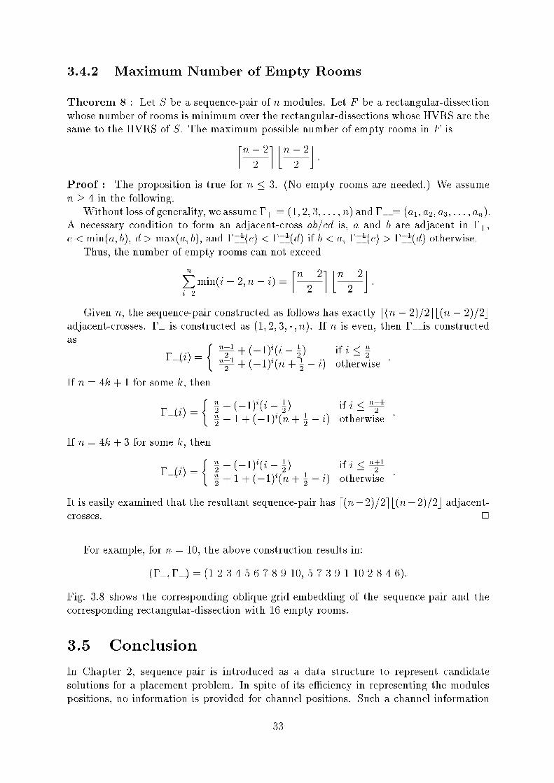
3.4.2 Maximum Number of Empty Rooms

Theorem 8 : Let S be a sequence-pair of n modules. Let F be a rectangular-dissection

whose number of rooms is minimum over the rectangular-dissections whose HVRS are the

same to the HVRS of S. The maximum possible number of empty rooms in F is

�n� 2

2

� �n� 2

2

�:

Proof : The proposition is true for n � 3. (No empty rooms are needed.) We assume

n � 4 in the following.

Without loss of generality, we assume �+ = (1; 2; 3; . . . ; n) and �� = (a1; a2; a3; . . . ; an).

A necessary condition to form an adjacent-cross ab=cd is, a and b are adjacent in �+,

c < min(a; b), d > max(a; b), and ��1� (c) < �

�1� (d) if b < a, ��1� (c) > �

�1� (d) otherwise.

Thus, the number of empty rooms can not exceed

nXi=2

min(i� 2; n� i) =

�n� 2

2

� �n� 2

2

�:

Given n, the sequence-pair constructed as follows has exactly d(n� 2)=2eb(n� 2)=2cadjacent-crosses. �+ is constructed as (1; 2; 3; ��; n). If n is even, then �� is constructed

as

��(i) =

(n+12

+ (�1)i(i� 1

2) if i � n

2

n+12

+ (�1)i(n+ 1

2� i) otherwise

:

If n = 4k + 1 for some k, then

��(i) =

(n2+ (�1)i(i� 1

2) if i � n�1

2

n2+ 1 + (�1)i(n+ 1

2� i) otherwise

:

If n = 4k + 3 for some k, then

��(i) =

(n2+ (�1)i(i� 1

2) if i � n+1

2

n2+ 1 + (�1)i(n+ 1

2� i) otherwise

:

It is easily examined that the resultant sequence-pair has d(n�2)=2eb(n�2)=2c adjacent-crosses. 2

For example, for n = 10, the above construction results in:

(�+;��) = (1 2 3 4 5 6 7 8 9 10, 5 7 3 9 1 10 2 8 4 6):

Fig. 3.8 shows the corresponding oblique-grid-embedding of the sequence-pair and the

corresponding rectangular-dissection with 16 empty rooms.

3.5 Conclusion

In Chapter 2, sequence-pair is introduced as a data structure to represent candidate

solutions for a placement problem. In spite of its e�ciency in representing the modules

positions, no information is provided for channel positions. Such a channel information

33

12 4

6

8

1097

5

3

6

8

7

5

3

1 24

109

Figure 3.8: Sequence-pair with maximum adjacent-crosses (left) and its corresponding

rectangular-dissection (right)

is added in this chapter by introducing a mapping from a sequence-pair to a rectangular-

dissection, which has been used to represent the channel positions together with the

module positions.

The result of this chapter is summarized as follows.

� Channels are additionally represented, without changing the information about

module positions, thus the following two properties of the sequence-pair are remain

e�ective; an area minimum placement is represented, and no overlapping placement

is represented.

� The number of channels is minimized, which most likely minimizes the number of

wire bends, later in the routing stage.

� The maximum possible number of empty rooms, which linearly corresponds to the

maximum possible number of introduced channels, is presented.

� A necessary and su�cient condition of the sequence-pair for not introducing any

empty-room is presented.

Although the channels are represented, this chapter does not give a technique to assign

width to each channel. How to assign adequate widths to the channels remains hard, and

would be solved heuristically.

34

Chapter 4

Rectangle Packing with Obstacles

4.1 Introduction

In VLSI design, it often happens that the locations of some macro cells, such as RAM,

ROM, and CPU core, are �xed a priori and the other components are subject to be placed

in the rest of the chip area. Also in PCB design, it is common that the exact coordinates

of connectors are determined before designing the placement of the other components.

We formulate such situations as a problem called \rectangle packing with pre-placed

rectangles (RPP)". Not only the circuit components but also rectangular obstacles in

any type are candidates to be modeled as pre-placed modules. For example, pre-placed

modules can be used for representing a rectilinear substrate and holes of the substrate.

The other \free" modules are requested to be placed onto the substrate without any

overlap with the pre-placed modules.

Chi [14] studied a similar but restricted problem, where all the free modules have

a regular height, assuming they are standard cells. Force-Directed-Relaxation method

(FDR) [6, 7] can be easily tailored to handle the obstacles, but the method has inherent

defects in the sensitiveness to the initial placement and in the incompleteness of the

overlap elimination. The most practical way would be to use a stochastic algorithm, such

as simulated annealing or genetic algorithm, if a proper coding scheme is available.

A coding technique for the slicing structure [8] is not useful for RPP, since the pre-

placed modules might be given non-slicibly. For general (including both slicible and

non-slicible) placements, we proposed the coding coding schemes called sequence-pair in

Chapter 2. Using the sequence-pair, it is easy to generate non-overlapping placements of

all the modules by encoding all the (free and pre-placed) modules, but the code could be

inconsistent to recover the locations of the pre-placed modules.

In this paper, we present a procedure called adaptation, which changes a sequence-pair

so that it becomes consistent to the pre-placed modules. The procedure only changes the

positions of pre-placed modules in a sequence-pair, and it runs in O(n2) time, where n

is the total number of pre-placed modules and free modules. The alternative ways to

incorporate the adaptation procedure in a simulated annealing are demonstrated through

experiments on an MCNC building block benchmark example, named ami49. The simu-

lated annealing is applied to a PCB example, with a standard wiring length estimation.

The resultant placement has turned out to be successfully routed by a commercial router.

The organization of this paper is as follows. Section 4.2 gives a formal de�nition of

RPP, and addresses that a sequence-pair can be inconsistent to RPP. In Section 4.3, the

35

Y

X

Figure 4.1: Feasible packing example. The dark rectangles are the pre-placed modules.

adaptation procedure is presented. Section 4.4 is devoted for the experiments. Section 4.5

is for conclusion.

4.2 Preliminary

4.2.1 Rectangle Packing with Pre-Placed Rectangles (RPP)

A module is a rectangle. A packing of a set of modules is a non-overlapping placement

of the modules. The coordinates of a module is the coordinates of the lower left corner

of the module. A pre-placed module is a module whose coordinates as well as width and

height are speci�ed. A free module is a module whose width and height are speci�ed but

the coordinates is not speci�ed. Set P of pre-placed modules is given such that no two

pre-placed modules overlap each other and all of them lie in the �rst quadrant of the

plane. Set F of free modules is also given. A feasible packing of P [ F is a packing of

P [ F on the �rst quadrant of the plane such that all the modules in P are placed at

their speci�ed locations. The evaluation of a feasible packing is the area of the minimum

bounding rectangle whose lower left corner is at the origin of the plane. Find the best

feasible packing of P [ F .

Fig. 4.1 shows a feasible packing of an instance of RPP.

When all the modules are free, i.e. P = ;, then RPP coincides with the packing

problem discussed in Chapter 2, denoted by RP, which is already proved to be NP-hard.Thus, RPP is also in NP-hard class.

4.2.2 Sequence-Pair

For the free packing problem (RP), a coding scheme is proposed in Chapter 2 as follows.

A sequence-pair for a set of n modules is a pair of sequences of the n module names.

For example, (abc; bac) is a sequence-pair for module set fa; b; cg. It is easily understood

that the variety of the sequence-pair for n modules is (n!)2.

36

a

bc

a

b c

(a) sequence-pair (abc; bac) (b) free-realization

Figure 4.2: Oblique grid notation of a sequence-pair and the free-realization of the

sequence-pair

A sequence-pair imposes a horizontal/vertical (H/V) constraint for every pair of mod-

ules, as follows.

(�� a ��b �� ; �� a ��b ��) ! a should be placed to the left of b

(�� b ��a �� ; �� a ��b ��) ! a should be placed below b

For example, sequence-pair (abc; bac) imposes a set of H/V constraints: f a should be

placed to the left of c, b should be placed to the left of c, b should be placed below ag.The H/V constraints of a sequence-pair can be intuitively grasped using the oblique-

grid notation. For example, Fig. 4.2(a) shows the oblique-grid of sequence-pair (abc; bac).

It is an n� n grid obliquely drawn on the plane, so constructed that the �rst sequence is

observed when one reads the module names on the positive slope lines from left to right,

and the second sequence is observed similarly with respect to the negative slope lines. It

shows the H/V constraints in such a way that: Modules c is in the right quarter view

range (between �45 degree and +45 degree) of module a, then c should be placed to the

right of a.

It is proved in Chapter 2 that: The set of H/V constraints imposed by every sequence-

pair is satis�able, and an area minimum packing under the constraint can be obtained

in polynomial time, and further, there is a sequence-pair which leads an (globally) area

minimum packing. Then, the sequence-pair is easily utilized as a coding scheme of a

stochastic algorithm.

To construct an area minimum placement for a sequence-pair, one dimensional com-

paction is carried out under the H/V constraints of the sequence-pair. The modules are

greedily pushed to the left, and to the bottom, as shown in Fig. 4.2(b). The resultant

placement is called the free-realization of the sequence-pair.

The free-realization can be obtained in O(n2) time 1by using the \H/V constraint

graph" which is constructed faithfully to the H/V constraints. More in detail: (Step 1)

1The time complexity is reduced to O(n log n) by Takahashi[22].

37

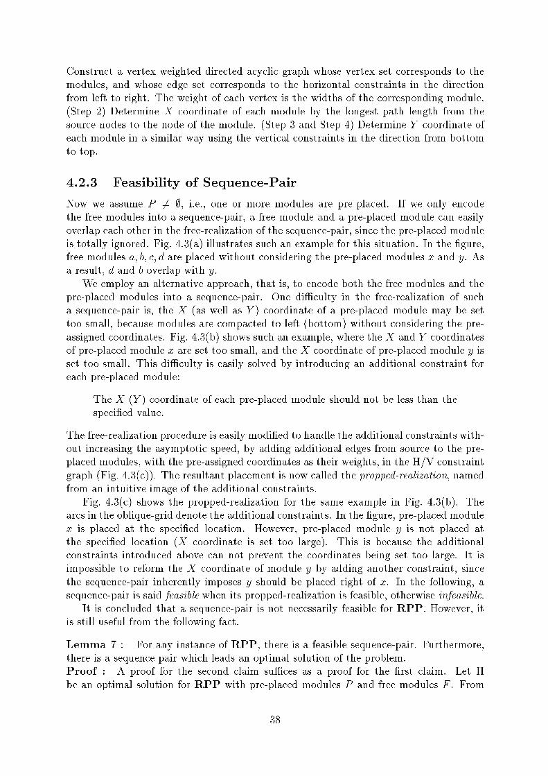
Construct a vertex weighted directed acyclic graph whose vertex set corresponds to the

modules, and whose edge set corresponds to the horizontal constraints in the direction

from left to right. The weight of each vertex is the widths of the corresponding module.

(Step 2) Determine X coordinate of each module by the longest path length from the

source nodes to the node of the module. (Step 3 and Step 4) Determine Y coordinate of

each module in a similar way using the vertical constraints in the direction from bottom

to top.

4.2.3 Feasibility of Sequence-Pair

Now we assume P 6= ;, i.e., one or more modules are pre-placed. If we only encode

the free modules into a sequence-pair, a free module and a pre-placed module can easily

overlap each other in the free-realization of the sequence-pair, since the pre-placed module

is totally ignored. Fig. 4.3(a) illustrates such an example for this situation. In the �gure,

free modules a; b; c; d are placed without considering the pre-placed modules x and y. As

a result, d and b overlap with y.

We employ an alternative approach, that is, to encode both the free modules and the

pre-placed modules into a sequence-pair. One di�culty in the free-realization of such

a sequence-pair is, the X (as well as Y ) coordinate of a pre-placed module may be set

too small, because modules are compacted to left (bottom) without considering the pre-

assigned coordinates. Fig. 4.3(b) shows such an example, where the X and Y coordinates

of pre-placed module x are set too small, and the X coordinate of pre-placed module y is

set too small. This di�culty is easily solved by introducing an additional constraint for

each pre-placed module:

The X (Y ) coordinate of each pre-placed module should not be less than the

speci�ed value.

The free-realization procedure is easily modi�ed to handle the additional constraints with-

out increasing the asymptotic speed, by adding additional edges from source to the pre-

placed modules, with the pre-assigned coordinates as their weights, in the H/V constraint

graph (Fig. 4.3(c)). The resultant placement is now called the propped-realization, named

from an intuitive image of the additional constraints.

Fig. 4.3(c) shows the propped-realization for the same example in Fig. 4.3(b). The

arcs in the oblique-grid denote the additional constraints. In the �gure, pre-placed module

x is placed at the speci�ed location. However, pre-placed module y is not placed at

the speci�ed location (X coordinate is set too large). This is because the additional

constraints introduced above can not prevent the coordinates being set too large. It is

impossible to reform the X coordinate of module y by adding another constraint, since

the sequence-pair inherently imposes y should be placed right of x. In the following, a

sequence-pair is said feasible when its propped-realization is feasible, otherwise infeasible.

It is concluded that a sequence-pair is not necessarily feasible for RPP. However, it

is still useful from the following fact.

Lemma 7 : For any instance of RPP, there is a feasible sequence-pair. Furthermore,

there is a sequence-pair which leads an optimal solution of the problem.

Proof : A proof for the second claim su�ces as a proof for the �rst claim. Let �

be an optimal solution for RPP with pre-placed modules P and free modules F . From

38

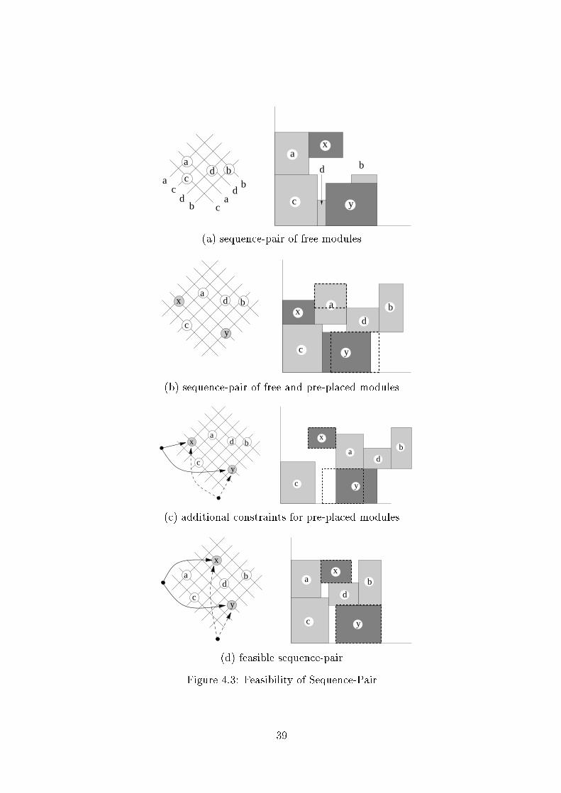
c

ax

y

bda

cd

b ca

db

c

ad b

(a) sequence-pair of free modules

x

yc

ba

d

c y

xa

d

b

(b) sequence-pair of free and pre-placed modules

c

x

y

x

yc

bda

ad

b

(c) additional constraints for pre-placed modules

c

x

y

d

a ba

y

x

db

c

(d) feasible sequence-pair

Figure 4.3: Feasibility of Sequence-Pair

39

Chapter 2, there is a sequence-pair S for P [F such that the length of every path between

two vertices in the H/V constraint graph is not greater than the di�erence between X/Y

coordinates of the modules in �, if the path consists of H/V constraint edges only. Since

the weight of each additional edge equals to the X (Y ) coordinate of the pre-placed

module, the length of every path between two vertices in the H/V constraint graph is not

greater than the di�erence between X (Y ) coordinates of the modules in �. Therefore,

in the propped-realization of S, we obtain a placement which is not worse than �, thus

also optimal. 2

Fig. 4.3(d) shows an example of a feasible (and optimal) sequence-pair and its propped-

realization.

4.3 Adaptation

Among (n!)2 sequence-pairs, there are feasible sequence-pairs, including one for optimal

solution of RPP, and infeasible sequence-pairs. We should consider how to treat the

infeasible sequence-pairs, when exploring the space by a stochastic algorithm. The easiest

way would be to evaluate them in�nitely negative, but the smoothness of the search would

be strongly weakened. To keep the smoothness as much as we can, it is desirable that

each infeasible sequence-pair is evaluated equally to a feasible sequence-pair which resem-

bles to the infeasible one. For this purpose, we present a procedure, called adaptation,

which transforms a given sequence-pair to a feasible sequence-pair, by changing only the

positions of pre-placed modules.

4.3.1 Necessary Condition

Suppose unit square modules a and b are pre-placed at (3; 3) and at (5; 5), respectively.

Then, both of \a is left of b" and \a is below b" are true, but \a is right of b" and \a is

above b" are both false. It turns out that a is necessary to appear before b in the second

sequence of a feasible sequence-pair. More in general, we describe a necessary condition

for the second sequence of a feasible sequence-pair.

For any two pre-placed modules a and b, we say that a dominates b if

x(a) < x(b) + w(b) and y(a) < y(b) + h(b)

where

� x(a); y(a) : X and Y coordinates of module a,

� w(a); h(a) : width and height of module a.

The domination relation introduces a partial order into the module set. Then, the

second sequence of a sequence-pair is said to be topologically sorted if it satis�es the

condition: If a dominates b, then a appears prior to b in the second sequence. It is clear

that the following lemma holds.

Lemma 8 : It is necessary for a sequence-pair being feasible that the second sequence

is topologically sorted. 2

40

4.3.2 Algorithm

In the propped-realization of a sequence-pair, the X and Y coordinates of a module is

determined only by the preceding modules in the second sequence. It turns out that the

coordinates of a module can be determined one by one, traversing the second sequence.

Then, we design our adaptation procedure so that it iteratively \test and virtually place"

a module according to the second sequence. Thus, after some iterations, free modules

would be virtually placed, as well as pre-placed modules. The relation \dominate" was

already de�ned for the pre-placed modules, but in the following, we use the relation also

for a free module when it is virtually placed.

Procedure Adaptation

Input: A set of pre-placed modules, a set of free modules, a sequence-pair.

Output: A feasible sequence-pair.

(Step 1) Topologically sort the second sequence, only when it is not already topologically

sorted.

(Step 2) For k = 1; 2; . . . ; n, repeat (Step 2.1) through (Step 2.4).

(Step 2.1) Let the k'th module in the second sequence be a. If module a is a pre-placed

module, go to (Step 2.4). Otherwise, temporary set the coordinates of a, according

to the propped-realization of a.

(Step 2.2) Determine whether there exists a pre-placed module which dominates a, in

the last n � k modules of the second sequence. When it exists, determine a pre-

placed module q such that q directly or transitively dominates a, and there is no

pre-placed module which dominates q. Otherwise, go to (Step 2) for the next

iteration.

(Step 2.3) In the second sequence, move q just before a. After that, a is used for referring

q. (since q is now the k'th module in the second sequence.)

(Step 2.4) If a is a free module, go to (Step 2) for the next iteration. Let (x; y) be

the coordinates of a in the propped-realization. Let (x(a); y(a)) be the speci�ed

coordinates of pre-placed module a. If x > x(a), then in the �rst sequence, move a

minimally toward the top so that x � x(a) holds. Otherwise, if y > y(a), then in

the �rst sequence, move a minimally toward the end so that y � y(a) holds.

(Procedure Adaptation End)

4.3.3 Illustrative Example

A behavioral example is presented for the RPP instance shown in Fig. 4.4(a), in which

the dark two modules x and y are pre-placed, and the rest of the modules a; b; c; d are

free.

Suppose sequence-pair (acdbyx; cadxyb) is given as the input sequence-pair. Fig. 4.4(b)

shows this initial sequence-pair. In (Step 1), x and y are exchanged in the second

sequence, and the sequence-pair becomes (acdbyx; cadyxb), as shown in Fig. 4.4(c).

41

ax’

bx

d’

dyc

a

cd

b

y

xac

db

yx c

ad

xy

b

(a) The packing example (b) (acdbyx; cadxyb)

a

cd

b

y xac

db

yx c

ad

b

yx

a

c

b

x

d

yac

db

yx c

a

bx

dy

(c) (acdbyx; cadyxb) (d) (acdbyx; caydxb)

a

y

x

db

ca

ca

bx

dy

x

yb

dc

(e) (axcdby; caydxb)

Figure 4.4: Snapshots of the adaptation procedure. (a) shows the packing corresponding

to the sequence-pair shown in (e). (b) shows the input sequence-pair. In (c), y is brought

before x in the second sequence. In (d), y is brought before d in the second sequence. In

(e), x is brought before c in the �rst sequence.

42

Now, (Step 2) begins. In iteration k = 1 and in k = 2, free modules c and a are

processed because they are the �rst and the second modules in the second sequence,

respectively. They are virtually placed at the positions shown in Fig. 4.4(a).

In iteration k = 3, module d is once tried to be placed at the right of c in (Step 2.1),

as indicated by the rectangle with dotted lines, which is marked \d" in Fig. 4.4(a). Then,

module y is selected in (Step 2.2), and it is brought before d in the second sequence

in (Step 2.3). As a result, the sequence-pair becomes (acdbyx; caydxb) as shown in

Fig. 4.4(d). Module y is virtually placed at its speci�ed position, as it is marked \y" in

Fig. 4.4(a).

In iteration k = 4, module d is placed at the position marked \d0"in Fig. 4.4(a).

In iteration k = 5, pre-placed module x is processed. In (Step 2.4), it is once tried to

placed at the position indicated by the rectangle with dotted lines, which is marked \x"

in Fig. 4.4(a), since it is the position imposed by the sequence-pair shown in Fig. 4.4(d).

Then, the X coordinate is found too large, and module x is moved toward the top of the

�rst sequence, and put between a and d. The sequence-pair becomes (axcdby; caydxb),

which is illustrated in Fig. 4.4(e). Module x is virtually placed at its speci�ed position,

as it is marked \x0" in Fig. 4.4(a).

This sequence-pair is not changed in iteration k = 6, and becomes the output of the

procedure.

One can examine on this example that the resultant sequence-pair is feasible. It is

important to note that the H/V constraints among the free modules are preserved.

4.3.4 Proof of Adaptation

Theorem 9 : The adaptation procedure changes the given sequence-pair such that

(1) the output sequence-pair coincides with the input sequence-pair if the given sequence-

pair is feasible,

(2) the output sequence-pair is always feasible,

(3) the H/V constraints with respect to the free modules are preserved,

(4) the procedure runs in O(n2) time, where n is the total number of the pre-placed

modules and the free modules.

Proof :

(1) and (3) are easily understood. (2) and (4) are proved in the following.

(2): Adaptation outputs a feasible sequence-pair.

LetMkdenote the set of �rst k modules in the second sequence of S. Let Sk

denote the

sequence-pair for Mkobtained from a sequence-pair S for M by deleting all the modules

in M �Mk.

When the k'th iteration starts in (Step 2), assume that the second sequence is topo-

logically sorted with respect to the domination relation between pre-placed modules, and

also assume that Sk�1is feasible (for Mk�1

). Both assumptions are satis�ed trivially for

k = 1. It is clear that (Step 2.1) through (Step 2.4) determines the k'th module in the

second sequence and its position in the �rst sequence without changing Sk�1. Then, it

43

su�ces as a proof if we show (Step 2.1) through (Step 2.4) produces a feasible Sk (for

Mk) in k'th iteration.

The proof is by contradiction. Assume k'th module a in the second sequence and

its position in the �rst sequence are determined in the k'th iteration, and Sk becomes

infeasible.

Module a should be a pre-placed module since Skcan not be made infeasible if a is a

free module.

It is also true that Sk can not be made infeasible if (Step 2.4) is successfully executed.

So, there must module b in Mk�1such that

x(a) < x(b) + w(b) and y(a) < y(b) + h(b):

If b is a pre-placed module, since b had been after a in the second sequence at the end

of (Step 1), it was brought before a afterward in (Step 2.3), in the iteration k0, where

k0 < k. In the iteration k0, the position of b in the second sequence was changed because

b is determined as module q in (Step 2.2), hence b is not dominated by any other

module. This contradicts to the fact that a dominates b. Then, b should be a free module

determined in the iteration k00. In the iteration k00, b is tested to be not dominated by

any pre-placed module in (Step 2.2). This contradicts to the fact that a dominates b.

Hence, it is concluded that Skis feasible. Therefore, the resultant sequence-pair obtained

by the procedure is feasible.

(4): The adaptation procedure can be run in O(n2) time.

(Step 1) can be done in O(n2) time as follows.

(a) Construct an n� n matrix D such that

D(a; b) =

8><>:

1 if module a directly or transitively

dominates b

0 otherwise

D can be constructed in O(n2) time by sorting the modules by their coordinates

in X and in Y , essentially because of the fact: If a transitively dominates b and

x(a) < x(b), then there is a series of modules from a to b, dominating one after

another, and their X coordinates are monotonically increasing.

(b) Topologically sort the second sequence using D. This can be done also in O(n2) time

by a selection sort algorithm.

(The claim is easily proved also by the ordinary depth �rst algorithm, but we use the

above algorithm with utmost consideration for minimizing the modi�cation.)

(Step 2.1) is easily done in O(n) time. (Step 2.2) can be done in O(n) time by

traversing the modules reversely in the second sequence. (Step 2.3) can be easily done

in O(n) time. (Step 2.4) can be done in O(n) time by introducing two arrays X[1 . . .n]

and Y [1 . . .n] which holds a \negative locus" (see Chapter 2) of the k'th module in the

second sequence after the module is virtually placed.

(Step 2.1) through (Step 2.4) is repeated n times in (Step 2). Therefore, the

adaptation can be done in O(n2) time. 2

44

4.4 Use of Adaptation

4.4.1 RPP Example

The adaptation procedure is implemented in a standard simulated annealing to solve

RPP. The outline of the simulated annealing is as follows.

Procedure SA

Input: Set P of pre-placed modules, set F of free modules, number of iterations, initial

temperature, and �nal temperature.

Output: A feasible packing of P [ F .(Step 1) Generate a random sequence-pair, initialize the loop counter, set temperature

to the initial value, and set the decreasing ratio of the temperature such that it

reaches to the �nal temperature when the loop counter reaches to the limit.

(Step 2) If the loop exceeds the given limit, output the best packing obtained so far and

then stop.

(Step 3) Apply one of the following three move operations to alter the sequence-pair.

� exchange two module names in the �rst sequence,

� exchange two module names both in the �rst sequence and the second sequence,

and

� exchange the width and the height of a module.

(Step 4) Evaluate the sequence-pair by the area of the corresponding placement.

(Step 5) If the evaluation is improved or not changed, then accept the change. Oth-

erwise, accept the change stochastically depending on the temperature and on the

di�erence of the evaluations.

(Step 6) Decrease the temperature exponentially by the ratio obtained in (Step 1), and

go to (Step 2).

(Procedure SA End)

The adaptation can be used in one of the following two manners:

� Adapt-in-Eval : Use the adaptation procedure internally in the evaluation step

(Step 4), intending to evaluate an infeasible sequence-pair as an equivalent of a

feasible sequence-pair.

� Adapt-in-Move : Use the adaptation procedure internally in the initialization step

(Step 1) and in the move step (Step 3) so that an infeasible sequence-pair is never

generated.

45

Figure 4.5: Three packings of ami49. The left �gure is obtained by RP. The middle

and the right �gures are obtained by Adapt-in-Eval method and Adapt-in-Move method,

respectively, setting the dark modules being pre-placed.

Table 4.1: An experimental result of ami49. (average of 10 runs)

RP Adapt-in-Eval Adapt-in-Move

Area (mm2) 37.978808 38.353762 40.062617

Time (sec) 331.78 1004.15 949.68

The major di�erence of the two methods would be as follows. In both methods, the

SA explores the space of (n!)2 sequence-pairs. Suppose there is a cluster of infeasible

sequence-pairs in the solution space. The search may go into the cluster in the Adapt-

in-Eval method, while in the Adapt-in-Move method, it is icked out from the cluster

right after an infeasible sequence-pair is generated eventually. Then, the reachability to

an optimal solution is guaranteed in the Adapt-in-Eval method, and not in the Adapt-in-

Move method.

The biggest MCNC building block benchmark example ami49 is used as the input

data. As a preliminary run, the 49 modules are all treated as free modules, and they

are packed by the simulated annealing. The �rst 10 biggest modules, with respect to the

areas, are speci�ed as pre-placed modules whose coordinates are �xed to those obtained

by the preliminary run. The reason why these modules are selected is because of our

experience that the obstacles are usually not many, but big. The same input, except

for the presence of the pre-placed modules, is applied to Adapt-in-Eval method and to

Adapt-in-Move method.

Fig. 4.5 shows the resultant packing of these methods, including the preliminary run.

Table 4.1 shows the average performance of 10 runs of the Adapt-in-Eval method, Adapt-

in-Move method, and also the preliminary run in the column RP for reference. Every

trial is performed on a Sun SS-5 (75 MHz).

The run time is shortest in RP, as in Table 4.1. This would be natural because the

adaptation is not executed, and also because (Step 4) runs in O(n log n) time when there

is no pre-placed modules, with an algorithm similar to [22]. The reason why Adapt-in-

Move runs faster than Adapt-in-Eval method would be because the input sequence-pair

46

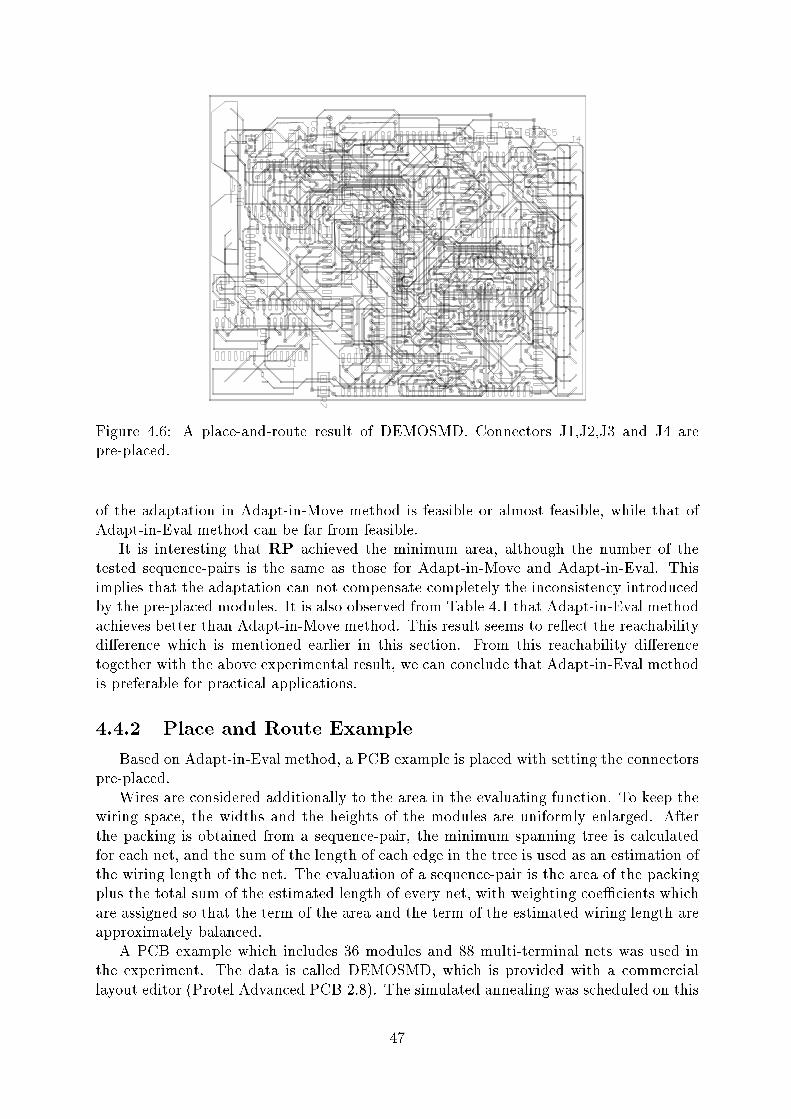
Figure 4.6: A place-and-route result of DEMOSMD. Connectors J1,J2,J3 and J4 are

pre-placed.

of the adaptation in Adapt-in-Move method is feasible or almost feasible, while that of

Adapt-in-Eval method can be far from feasible.

It is interesting that RP achieved the minimum area, although the number of the

tested sequence-pairs is the same as those for Adapt-in-Move and Adapt-in-Eval. This

implies that the adaptation can not compensate completely the inconsistency introduced

by the pre-placed modules. It is also observed from Table 4.1 that Adapt-in-Eval method

achieves better than Adapt-in-Move method. This result seems to re ect the reachability

di�erence which is mentioned earlier in this section. From this reachability di�erence

together with the above experimental result, we can conclude that Adapt-in-Eval method

is preferable for practical applications.

4.4.2 Place and Route Example

Based on Adapt-in-Eval method, a PCB example is placed with setting the connectors

pre-placed.

Wires are considered additionally to the area in the evaluating function. To keep the

wiring space, the widths and the heights of the modules are uniformly enlarged. After

the packing is obtained from a sequence-pair, the minimum spanning tree is calculated

for each net, and the sum of the length of each edge in the tree is used as an estimation of

the wiring length of the net. The evaluation of a sequence-pair is the area of the packing

plus the total sum of the estimated length of every net, with weighting coe�cients which

are assigned so that the term of the area and the term of the estimated wiring length are

approximately balanced.

A PCB example which includes 36 modules and 88 multi-terminal nets was used in

the experiment. The data is called DEMOSMD, which is provided with a commercial

layout editor (Protel Advanced PCB 2.8). The simulated annealing was scheduled on this

47

Table 4.2: An experimental result of DEMOSMD

MST MBOX

Total wiring length (mm) 7,914.64 8,188.96

Number of vias 368 382

Placement time (sec.) 630 150

Routing time (sec.) 568 590

Total time (sec.) 1,198 740

data to try 100; 000 moves, on a note-type personal computer (Sharp Mebius PC-A355,

Pentium 100MHz). The resultant placement was given to a commercial router (Protel

AdvancedRoute3) to �nish the design using 4 layers.

All the nets were successfully routed, as shown in Fig. 4.6. The performance is sum-

marized in Table 4.2, in the column labeled with \MST".

By replacing the MST estimation with the half perimeter of the minimum bounding

box, which is a popular way to speed up the estimation, the same trial was carried out and

also completely routed by the router. Results are in Table 4.2, in the \MBOX" column.

4.5 Conclusion

We showed that the presence of the pre-placed modules introduces an inconsistency to

the sequence-pair coding scheme. An adaptation procedure is proposed to transform an

inconsistent sequence-pair to a consistent one. It is shown that a simulated annealing is

well organized to test only feasible placements with this adaptation procedure. A PCB

example is placed with a standard wiring estimation, and is routed successfully by a

commercial router.

48

Chapter 5

Conclusion

The motivation for this work was our experience that many VLSI designers are not satis-

�ed with the slicing structure and that many PCB designers place the modules manually.

To break-though this di�culty, a fundamental rectangle packing problem is investigated

in this thesis.

The major contribution of this thesis is to present a representation of a general packing

in terms of a pair of module name sequences, called sequence-pair. Detailed proofs are

presented to show that every sequence-pair feasibly corresponds to a packing, and at least

one sequence-pair corresponds to an area-minimum packing.

In experiments, 500 rectangles were packed very e�ciently in a reasonable time. It was

attained by a standard simulated annealing in which a move is a change of the sequence-

pair. The evaluating function was then extended to the VLSI placement problem using a

conventional wiring area estimation method. It shows such a performance that the biggest

MCNC benchmark, ami49, is placed promisingly.

Another e�ort is devoted to �ll in the gap between the fundamental packing problem

and the practical placement problems. In practice, there are various additional criteria and

constraints besides the basic criterion of packing (chip area). This thesis gives methods

for two of those topics, channel generation and placement with obstacles.

New VLSI technologies are o�ering a su�cient number of layers for routing to allow

enough space for routing to be done on top of the modules, assuming the use of some

\area router". This technology trend will bring placement design still closer to packing,

hence make our approach more signi�cant.

However, practical layout in VLSI/PCB is processed under various constraints and

di�erent objectives. For example, wire congestion estimation, timing, power dissipation,

clock distribution, crosstalk, are crucial to consider. To include them in our pure packing

algorithm, many studies on real instances and theories are necessary, which are left for

future researches.

49

Bibliography

[1] B. S. Baker, E. G. Co�man, and R. L. Rivest, \Orthogonal Packings in Two Dimen-

sions," SIAM J. Comput., vol. 9, no. 4, pp. 846{855, 1980.

[2] I. Golan, \Performance Bounds for Orthogonal Oriented Two-Dimensional Packing

Algorithms," SIAM J. Comput., vol. 10, no. 3, 1981.

[3] B. S. Baker, D. J. Brown, and H. P. Katse�, \A 5=4 Algorithm for Two-Dimensional

Packing," Journal of Algorithms, vol. 2, pp. 348{368, 1981.

[4] E. G. Co�man and J. C. Lagarias, \Algorithms for Packing Squares: A Probabilistic

Analysis," SIAM J. Comput., vol. 18, no. 1, pp. 166{185, 1989.

[5] I. Schiermeyer, \Reverse-Fit: A 2-optimal Algorithm for Packing Rectangles,"

ESA'94 Algorithms: Lecture Notes in Computer Science, vol. 855, pp. 290{299, 1994.

[6] L. Sha and R. W. Dutton, \An Analytical Algorithm for Placement of Arbitrarily

Sized Rectangular Blocks," in Proc. 22th ACM/IEEE Design Automation Conf.,

pp. 602{608, 1985.

[7] A. Alon and U. Ascher, \Model and Solution Strategy for Placement of Rectangular

Blocks in the Euclidean Plane," IEEE Trans. on CAD, vol. 7, no. 3, pp. 378{386,

1988.

[8] D. F. Wong and C. L. Liu, \A New Algorithm for Floorplan Designs," in Proc. 23rd

ACM/IEEE Design Automation Conf., pp. 101{107, 1986.

[9] H. Esbensen and E. S. Kuh, \An MCM/IC Timing-Driven Placement Algorithm Fea-

turing Explicit Design Space Exploration," in Proc. of the IEEE Multi-Chip Module

Conference, pp. 170{175, 1996.

[10] R. H. J. M. Otten, \Automatic Floorplan Design," in Proc. 19th ACM/IEEE Design

Automation Conf., pp. 261{267, 1982.

[11] T. C. Wang and D. F. Wong, \An Optimal Algorithm for Floorplan Area Optimiza-

tion," in Proc. 27th ACM/IEEE Design Automation Conf., pp. 180{186, 1990.

[12] W. M. Dai and E. Kuh, \Simultaneous Floorplanning and Global Routing for Hierar-

chical Building Block Layout," IEEE Trans. on CAD, vol. CAD-6, no. 5, pp. 828{837,

1987.

[13] H. Onodera, Y. Taniguchi, and K. Tamaru, \Branch-and-Bound Placement for Build-

ing Block Layout," in Proc. 28th ACM/IEEE Design Automation Conf., pp. 433{439,

1991.

50

[14] M. C. Chi, \An Automatic Rectilinear Partitioning Procedure for Standard Cells,"

in 24th ACM/IEEE Design Automation Conference, pp. 50{55, 1987.

[15] Y. Kajitani, \|," in personal communication, 1997.

[16] Y. Kajitani, \Order of Channels for Safe Routing and Optimal Compaction of Rout-

ing Area," IEEE Trans. on CAD, vol. 2, no. 4, pp. 293{300, 1983.

[17] L. Stockmeyer, \Optimal Orientations of Cells in Slicing Floorplan Designs," Infor-

mation and Control, vol. 59, pp. 91{101, 1983.

[18] P. Pan, W. Shi, and C. L. Liu, \Area Minimization for Hierarchical Floorplans," in

IEEE International Conf. on Computer Aided Design, pp. 436{440, 1994.

[19] M. J. Ciesielski and E. Kinnen, \Digraph Relaxation for 2-Dimensional Placement

of IC Blocks," IEEE Trans. on CAD, vol. CAD-6, no. 1, pp. 55{66, 1987.

[20] S. M.Sait and H. Youssef, VLSI Physical Design Automation. IEEE Press, 1995.

[21] S. Wimer, I. Koren, and I. Cederbaum, \Floorplans, Planar Graphs, and Layouts,"

IEEE Trans. Circuits & Syst., vol. 35, no. 3, pp. 267{278, 1988.

[22] T. Takahashi, \An Algorithm for Finding a Maximum-Weight Decreasing Sequence

in a Permutation, Motivated by Rectangle Packing Problem," Technical Report of

IEICE, vol. VLD96, no. 201, pp. 31{35, 1996.

51

Publications

[1] S. Nakatake, H. Murata, K. Fujiyoshi, and Y. Kajitani, \Bounded-Slicing Structure

for Module Placement", Technical Report of IEICE, Vol. VLD94, No. 313, pp.19{

24, 1994.

[2] H. Murata, K. Fujiyoshi, S. Nakatake, and Y. Kajitani, \A Solution Space of Size

(n!)2 for Optimal Rectangle Packings", 8th IEICE Circuit and Systems Karuizawa

Workshop, pp.109{114, 1995.

[3] H. Murata, K. Fujiyoshi, S. Nakatake, and Y. Kajitani, \Rectangle-Packing-Based

Module Placement", 1995 IEEE/ACM International Conference on Computer-Aided

Design, pp.472{479, 1995.

[4] T. Watanabe, H. Murata, and K. Fujiyoshi, \An Optimal Floorplan with Mod-

ule Relations Represented by a Sequence-Pair", 9th IEICE Circuit and Systems

Karuizawa Workshop, pp.103{108, 1996.

[5] S. Nakatake, K. Fujiyoshi, H. Murata, and Y. Kajitani, \Module Placement on BSG-

Structure and IC Layout Applications", 1996 IEEE/ACM International Conference

on Computer-Aided Design, pp. 484{491, 1996.

[6] H. Murata, K. Fujiyoshi, S. Nakatake, and Y. Kajitani, \VLSI Module Place-

ment Based on Rectangular-Packing by the Sequence-Pair", IEEE Transactions

on Computer-Aided Design of Integrated Circuits and Systems, Vol. 15, No. 12,

pp.1518{1524, Dec. 1996.

[7] H. Murata, K. Fujiyoshi, T. Watanabe, and Y. Kajitani, \AMapping from Sequence-

Pair to Rectangular Dissection", Asia and South Paci�c Design Automation Con-

ference, pp. 625{633, Jan. 1997.

[8] H. Murata, K. Fujiyoshi, and M. Kaneko, \VLSI/PCB Module Placement with Ob-

stacles Based on Sequence-Pair", 1997 International Symposium on Physical Design,

Apr. 1997. (to appear)

52