
孔令傑 / 給工程師的統計學及資料分析 123 (2016/9/4)
253
Basic concepts Data visualization Data summarization Statistics and Data Analysis for Engineers Part 1: Introduction and Descriptive Statistics Ling-Chieh Kung Department of Information Management National Taiwan University September 4, 2016 Introduction and Descriptive Statistics 1 / 62 Ling-Chieh Kung (NTU IM)
-
date post
21-Apr-2017 -
Category
Data & Analytics
-
view
10.564 -
download
0
Transcript of 孔令傑 / 給工程師的統計學及資料分析 123 (2016/9/4)
Basic concepts Data visualization Data summarization
Statistics and Data Analysis for Engineers
Part 1:Introduction and Descriptive Statistics
Ling-Chieh Kung
Department of Information ManagementNational Taiwan University
September 4, 2016
Introduction and Descriptive Statistics 1 / 62 Ling-Chieh Kung (NTU IM)

Basic concepts Data visualization Data summarization
What is Statistics?
I Many things are unknown...I Consumers’ tastes.I Quality of a product.I Stock prices.I The effectiveness of a new way of teaching/training.
I Statistics is the science of collecting, analyzing, interpreting, andpresenting (numerical) data.I Ultimate goal (of Business Statistics): to achieve better decision making.
I The study of Statistics includes:I Descriptive Statistics.I Probability.I Inferential Statistics: Estimation.I Inferential Statistics: Hypothesis testing.I Inferential Statistics: Prediction.
I In summary: To estimate, test, and predict those unknowns.
Introduction and Descriptive Statistics 2 / 62 Ling-Chieh Kung (NTU IM)

Basic concepts Data visualization Data summarization
My plan for today
I Descriptive Statistics.I Visualization and summarization.
I Inferential Statistics.I (Probability).I Hypothesis testing and p-value.I Regression analysis.
I Case studies.
Introduction and Descriptive Statistics 3 / 62 Ling-Chieh Kung (NTU IM)
Basic concepts Data visualization Data summarization
Road map
I Basic concepts.
I Data visualization.
I Data summarization.
Introduction and Descriptive Statistics 4 / 62 Ling-Chieh Kung (NTU IM)

Basic concepts Data visualization Data summarization
Populations vs. samples
I A population is a collection of persons, objects, or items.I A census is to investigate the whole population.
I A sample is a portion of the population.I Sampling is to investigate only a subset of the population.I We then use the information contained in the sample to infer (“guess”)
about the population.
I What are samples for the following populations?I All students in NTU.I All students in the business school.I All chips made in one factory.I All consumers who have bought iPhone 6.
I Two important questions:I Why sampling?I Is a sample representative?
Introduction and Descriptive Statistics 5 / 62 Ling-Chieh Kung (NTU IM)
Basic concepts Data visualization Data summarization
Descriptive vs. inferential statistics
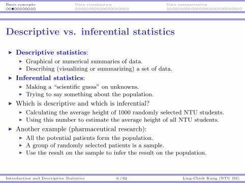
I Descriptive statistics:I Graphical or numerical summaries of data.I Describing (visualizing or summarizing) a set of data.
I Inferential statistics:I Making a “scientific guess” on unknowns.I Trying to say something about the population.
I Which is descriptive and which is inferential?I Calculating the average height of 1000 randomly selected NTU students.I Using this number to estimate the average height of all NTU students.
I Another example (pharmaceutical research):I All the potential patients form the population.I A group of randomly selected patients is a sample.I Use the result on the sample to infer the result on the population.
Introduction and Descriptive Statistics 6 / 62 Ling-Chieh Kung (NTU IM)
Basic concepts Data visualization Data summarization
Parameters vs. statistics
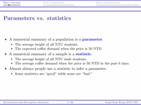
I A numerical summary of a population is a parameter.I The average height of all NTU students.I The expected coffee demand when the price is 50 NTD.
I A numerical summary of a sample is a statistic.I The average height of all NTU male students.I The average coffee demand when the price is 50 NTD in the past 6 days.
I Almost always people use a statistic to infer a parameter.I Some statistics are “good” while some are “bad.”
Introduction and Descriptive Statistics 7 / 62 Ling-Chieh Kung (NTU IM)
Basic concepts Data visualization Data summarization
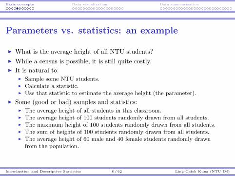
Parameters vs. statistics: an example
I What is the average height of all NTU students?
I While a census is possible, it is still quite costly.
I It is natural to:I Sample some NTU students.I Calculate a statistic.I Use that statistic to estimate the average height (the parameter).
I Some (good or bad) samples and statistics:I The average height of all students in this classroom.I The average height of 100 students randomly drawn from all students.I The maximum height of 100 students randomly drawn from all students.I The sum of heights of 100 students randomly drawn from all students.I The average height of 60 male and 40 female students randomly drawn
from the population.
Introduction and Descriptive Statistics 8 / 62 Ling-Chieh Kung (NTU IM)
Basic concepts Data visualization Data summarization
Levels of data measurement
I Most data we will play with are numerical.
I Numerical data may be categorized to three levels:I Nominal.I Ordinal.I Quantitative: interval or ratio.
Introduction and Descriptive Statistics 9 / 62 Ling-Chieh Kung (NTU IM)

Basic concepts Data visualization Data summarization
Nominal level
I A nominal scale classifies data into categories with no ranking.
I Data are labels or names used to identify an attribute of the element.
I The label may be numeric or non-numeric label.
I Examples:
Categorical variables Values (Categories)
Laptop ownership Yes / NoCitizenship Taiwan / Japan / ...Country code 886 / 86 / 1 / ...
I Arithmetic operations cannot be applied on nominal data.
Introduction and Descriptive Statistics 10 / 62 Ling-Chieh Kung (NTU IM)
Basic concepts Data visualization Data summarization
Ordinal level
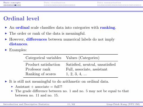
I An ordinal scale classifies data into categories with ranking.
I The order or rank of the data is meaningful.
I However, differences between numerical labels do not implydistances.
I Examples:
Categorical variables Values (Categories)
Product satisfaction Satisfied, neutral, unsatisfiedProfessor rank Full, associate, assistantRanking of scores 1, 2, 3, 4, ...
I It is still not meaningful to do arithmetic on ordinal data.I Assistant + associate = full?!I The grade difference between no. 1 and no. 5 may not be equal to that
between no. 11 and no. 15.
Introduction and Descriptive Statistics 11 / 62 Ling-Chieh Kung (NTU IM)

Basic concepts Data visualization Data summarization
Quantitative (interval and ratio) levels
I An interval scale is an ordered scale in which the difference betweenmeasurements is a meaningful quantity but the measurements do nothave a true zero point.
I A ratio scale is an ordered scale in which the difference betweenmeasurements is a meaningful quantity and the measurements have atrue zero point.
I Ratio data appear more often in the world.I Heights, weights, income, prices.
I Interval data are actually rare.I Degrees in Celsius or Fahrenheit.I GRE or GMAT scores.
I How about degrees in Kelvin?
Introduction and Descriptive Statistics 12 / 62 Ling-Chieh Kung (NTU IM)

Basic concepts Data visualization Data summarization
Some remarks
I Nominal and ordinal data are called qualitative data.
I Interval and ratio data are called quantitative data.
I Most statistical methods are for quantitative data; some are forqualitative data.I Distinguishing nominal and ordinal scales is important.I Distinguishing interval and ratio scales is not.
I Sometimes qualitative data are called categorical data.
I Sometimes quantitative data are called numeric data.
Introduction and Descriptive Statistics 13 / 62 Ling-Chieh Kung (NTU IM)

Basic concepts Data visualization Data summarization
A short summary
I Understand these terms:
I Populations vs. samples.I Parameters vs. statistics.I Inferential statistics vs. descriptive statistics.
I For each scale of measurement, is it meaningful to calculate thefollowing numbers?
Level Ranking Distance
Nominal No NoOrdinal Yes NoQuantitative Yes Yes
Introduction and Descriptive Statistics 14 / 62 Ling-Chieh Kung (NTU IM)

Basic concepts Data visualization Data summarization
Road map
I Basic concepts.
I Data visualization.
I Data summarization.
Introduction and Descriptive Statistics 15 / 62 Ling-Chieh Kung (NTU IM)

Basic concepts Data visualization Data summarization
An example
I For each day in 2011 and 2012, we recordthe number of daily rentals of the publicbike rental system in Washington, D.C.I 985, 801, 1349, 1562, 1600, 1606, 1510, ...,
1341, 1796. and 2729.I The smallest and largest numbers are 22
and 8714, respectively.
I How to get some feeling on 731 numbers?
date rental
2011/1/1 9852011/1/2 8012011/1/3 13492011/1/4 15622011/1/5 16002011/1/6 16062011/1/7 1510
...
2012/12/29 13412012/12/30 17962012/12/31 2729
Introduction and Descriptive Statistics 16 / 62 Ling-Chieh Kung (NTU IM)
Basic concepts Data visualization Data summarization
Frequency distributions
I The original 731 numbers form a set of ungrouped data.
I We start by grouping them into a frequency distribution.I Grouped data presented in the form of class intervals and frequencies.
I Let’s create an intuitive frequency distribution.
Introduction and Descriptive Statistics 17 / 62 Ling-Chieh Kung (NTU IM)

Basic concepts Data visualization Data summarization
Frequency distributions: an example
I The resulting classes:
Class Class interval (Which means)
1 [0, 1000) 0 ≤ x < 10002 [1000, 2000) 1000 ≤ x < 20003 [2000, 3000) 2000 ≤ x < 3000
...8 [7000, 8000) 7000 ≤ x < 80009 [8000, 9000) 8000 ≤ x < 9000
I How about [0, 999], [1000, 1999], etc.?I How about (0, 1000], (1000, 2000], etc.?
Introduction and Descriptive Statistics 18 / 62 Ling-Chieh Kung (NTU IM)

Basic concepts Data visualization Data summarization
Frequency distributions: an example
I Then we count to get the frequencydistribution at the right.
I This is a set of grouped data.
I Some remarks:I Typically we have 5 to 15 classes.I Typically all classes have the same
width.I Be aware of class endpoints! Classes
should NOT overlap with each other.I If there are outliers, they should be
removed first.
Class interval Frequency
[0, 1000) 18[1000, 2000) 80[2000, 3000) 74[3000, 4000) 107[4000, 5000) 166[5000, 6000) 106[6000, 7000) 86[7000, 8000) 82[8000, 9000) 12
Introduction and Descriptive Statistics 19 / 62 Ling-Chieh Kung (NTU IM)
Basic concepts Data visualization Data summarization
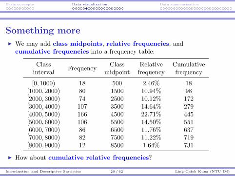
Something moreI We may add class midpoints, relative frequencies, and
cumulative frequencies into a frequency table:
ClassFrequency
Class Relative Cumulativeinterval midpoint frequency frequency
[0, 1000) 18 500 2.46% 18[1000, 2000) 80 1500 10.94% 98[2000, 3000) 74 2500 10.12% 172[3000, 4000) 107 3500 14.64% 279[4000, 5000) 166 4500 22.71% 445[5000, 6000) 106 5500 14.50% 551[6000, 7000) 86 6500 11.76% 637[7000, 8000) 82 7500 11.22% 719[8000, 9000) 12 8500 1.64% 731
I How about cumulative relative frequencies?
Introduction and Descriptive Statistics 20 / 62 Ling-Chieh Kung (NTU IM)

Basic concepts Data visualization Data summarization
Histograms
I A frequency distribution may be depicted as a histogram.
Interval Freq.
[0, 1000) 18[1000, 2000) 80[2000, 3000) 74[3000, 4000) 107[4000, 5000) 166[5000, 6000) 106[6000, 7000) 86[7000, 8000) 82[8000, 9000) 12
I It consists of a series of contiguous rectangles, each representing thefrequency in a class.
Introduction and Descriptive Statistics 21 / 62 Ling-Chieh Kung (NTU IM)
Basic concepts Data visualization Data summarization
Histograms
I Histograms may be the most important type of data graphs.
I One particular reason to draw histograms is to get some ideas aboutthe distribution.I Bell shape? M shape? Skewed?I Any outlier?I We will discuss distributions in more details.
Introduction and Descriptive Statistics 22 / 62 Ling-Chieh Kung (NTU IM)

Basic concepts Data visualization Data summarization
Frequency polygons
I Alternatively, we may draw a frequency polygon by using linesegments connecting dots plotted at class midpoints.I The information contained in a frequency polygon is quite similar to that
contained in a histogram.
Introduction and Descriptive Statistics 23 / 62 Ling-Chieh Kung (NTU IM)
Basic concepts Data visualization Data summarization
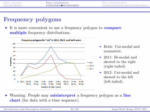
Frequency polygonsI It is more convenient to use a frequency polygon to compare
multiple frequency distributions.
I Both: Uni-modal andsymmetric.
I 2011: Bi-modal andskewed to the right(right-tailed).
I 2012: Uni-modal andskewed to the left(left-tailed).
I Warning: People may misinterpret a frequency polygon as a linechart (for data with a time sequence).
Introduction and Descriptive Statistics 24 / 62 Ling-Chieh Kung (NTU IM)

Basic concepts Data visualization Data summarization
Line chartsI A line chart is useful in depicting a time series data set.
I A two-dimensional data set whose first dimension (the x-axis) is forlabels of time points.
I It visualizes how a quantity changes as time goes by.I For our monthly bike rentals:
Introduction and Descriptive Statistics 25 / 62 Ling-Chieh Kung (NTU IM)

Basic concepts Data visualization Data summarization
Pie charts
I A pie chart is a circular depiction of data where each slice representsthe percentage of the corresponding category.
I It visualizes relative frequency distributions well.
I For our bike rental data set:I What are the proportions of rentals in the four seasons?I What are the proportions of rentals on the seven days of a week?
Introduction and Descriptive Statistics 26 / 62 Ling-Chieh Kung (NTU IM)

Basic concepts Data visualization Data summarization
A pie chart for seasonal rentals
Season Total rentals Proportion
Winter (12/20-3/20) 471348 14.3%Spring (3/21-6/20) 918589 27.9%Summer (6/21-9/20) 1061129 32.2%Fall (9/21-12/20) 841613 25.6%
Introduction and Descriptive Statistics 27 / 62 Ling-Chieh Kung (NTU IM)

Basic concepts Data visualization Data summarization
A pie chart for rentals among weekdays
Day Total rentals
Sunday 444027Monday 455503Tuesday 469109
Wednesday 473048Thursday 485395Friday 487790
Saturday 477807
Introduction and Descriptive Statistics 28 / 62 Ling-Chieh Kung (NTU IM)
Basic concepts Data visualization Data summarization
Data not appropriate for pie charts
I Pie charts are used to visualize proportions, i.e., subtotals over theoverall total.
I It should not be used to compare averages.I The total numbers of rentals made by male and female users are
appropriate for a pie chart.I The average numbers of rentals per male and female users are not
appropriate for a pie chart.
Introduction and Descriptive Statistics 29 / 62 Ling-Chieh Kung (NTU IM)

Basic concepts Data visualization Data summarization
Bar charts
I Pie charts are useful in visualizing the proportions of each categories.
I In demonstrating the differences among categories, a bar chart is abetter choice.I The larger the category, the longer the bar.I Some people draw bars vertically; some horizontally.
Introduction and Descriptive Statistics 30 / 62 Ling-Chieh Kung (NTU IM)

Basic concepts Data visualization Data summarization
Bar charts
I Let’s replace the pie chart to a bar chart.
Day Total rentals
Sunday 444027Monday 455503Tuesday 469109
Wednesday 473048Thursday 485395Friday 487790
Saturday 477807
I Note that the y-axis does not start at 0!
Introduction and Descriptive Statistics 31 / 62 Ling-Chieh Kung (NTU IM)

Basic concepts Data visualization Data summarization
Bar charts v.s. histograms
I What are the differences that distinguish a bar chart from a histogram?
I A bar chart uses noncontiguous bars to visualize categorical data.I A histogram uses contiguous bars to visualize quantitative data.
Introduction and Descriptive Statistics 32 / 62 Ling-Chieh Kung (NTU IM)
Basic concepts Data visualization Data summarization
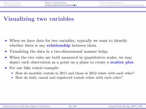
Visualizing two variables
I When we have data for two variables, typically we want to identifywhether there is any relationship between them.
I Visualizing the data in a two-dimensional manner helps.
I When the two vales are both measured in quantitative scales, we maydepict each observation as a point on a plane to create a scatter plot.
I For our bike rental example:I How do monthly rentals in 2011 and those in 2012 relate with each other?I How do daily casual and registered rentals relate with each other?
Introduction and Descriptive Statistics 33 / 62 Ling-Chieh Kung (NTU IM)

Basic concepts Data visualization Data summarization
Monthly rentals in 2011 and 2012
Month 2011 2012
1 38189 967442 48215 1031373 64045 1648754 94870 1742245 135821 1958656 143512 2028307 141341 2036078 136691 2145039 127418 21857310 123511 19884111 102167 15266412 87323 123713
Introduction and Descriptive Statistics 34 / 62 Ling-Chieh Kung (NTU IM)

Basic concepts Data visualization Data summarization
Road map
I Basic concepts.
I Data visualization.
I Data summarization.
Introduction and Descriptive Statistics 35 / 62 Ling-Chieh Kung (NTU IM)
Basic concepts Data visualization Data summarization
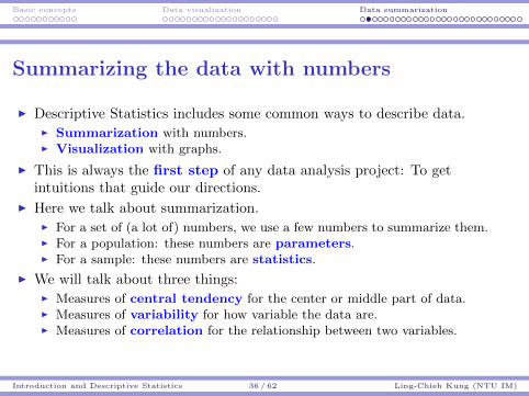
Summarizing the data with numbers
I Descriptive Statistics includes some common ways to describe data.I Summarization with numbers.I Visualization with graphs.
I This is always the first step of any data analysis project: To getintuitions that guide our directions.
I Here we talk about summarization.I For a set of (a lot of) numbers, we use a few numbers to summarize them.I For a population: these numbers are parameters.I For a sample: these numbers are statistics.
I We will talk about three things:I Measures of central tendency for the center or middle part of data.I Measures of variability for how variable the data are.I Measures of correlation for the relationship between two variables.
Introduction and Descriptive Statistics 36 / 62 Ling-Chieh Kung (NTU IM)

Basic concepts Data visualization Data summarization
Medians
I The median is the middle value in an ordered set of numbers.I Roughly speaking, half of the numbers are below and half are above it.
I Suppose there are N numbers:I If N is odd, the median is the N+1
2th large number.
I If N is even, the median is the average of the N2
th and the (N2
+ 1)thlarge number.
I For example:I The median of {1, 2, 4, 5, 6, 8, 9} is 5.I The median of {1, 2, 4, 5, 6, 8} is 4+5
2= 4.5.
Introduction and Descriptive Statistics 37 / 62 Ling-Chieh Kung (NTU IM)

Basic concepts Data visualization Data summarization
Medians
I A median is unaffected by the magnitude of extreme values:I The median of {1, 2, 4, 5, 6, 8, 9} is 5.I The median of {1, 2, 4, 5, 6, 8, 900} is still 5.
I Medians may be calculated from quantitative or ordinal data.I It cannot be calculated from nominal data.
I Unfortunately, a median uses only part of the information contained inthese numbers.I For quantitative data, a median only treats them as ordinal.
Introduction and Descriptive Statistics 38 / 62 Ling-Chieh Kung (NTU IM)
Basic concepts Data visualization Data summarization
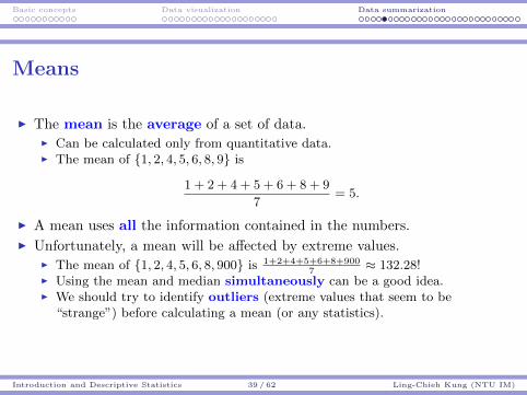
Means
I The mean is the average of a set of data.I Can be calculated only from quantitative data.I The mean of {1, 2, 4, 5, 6, 8, 9} is
1 + 2 + 4 + 5 + 6 + 8 + 9
7= 5.
I A mean uses all the information contained in the numbers.
I Unfortunately, a mean will be affected by extreme values.I The mean of {1, 2, 4, 5, 6, 8, 900} is 1+2+4+5+6+8+900
7≈ 132.28!
I Using the mean and median simultaneously can be a good idea.I We should try to identify outliers (extreme values that seem to be
“strange”) before calculating a mean (or any statistics).
Introduction and Descriptive Statistics 39 / 62 Ling-Chieh Kung (NTU IM)
Basic concepts Data visualization Data summarization
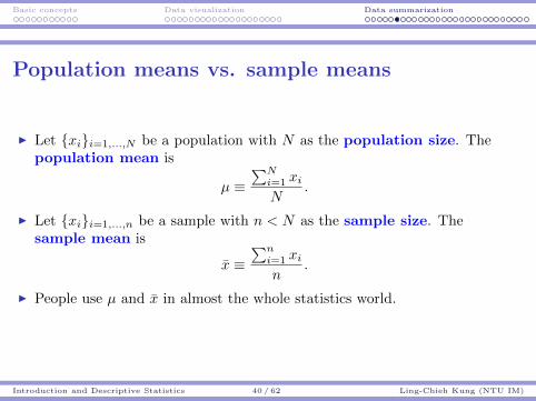
Population means vs. sample means
I Let {xi}i=1,...,N be a population with N as the population size. Thepopulation mean is
µ ≡∑N
i=1 xiN
.
I Let {xi}i=1,...,n be a sample with n < N as the sample size. Thesample mean is
x ≡∑n
i=1 xin
.
I People use µ and x in almost the whole statistics world.
Introduction and Descriptive Statistics 40 / 62 Ling-Chieh Kung (NTU IM)

Basic concepts Data visualization Data summarization
Population means v.s. sample means
µ ≡∑N
i=1 xiN
x ≡∑n
i=1 xin
.
I Isn’t these two means the same?I From the perspective of calculation, yes.I From the perspective of statistical inference, no.
I Typically the population mean is fixed but unknown.I The sample mean is random: We may get different values of x today
and tomorrow.I To start from x and use inferential statistics to estimate or test µ, we
need to apply probability.
Introduction and Descriptive Statistics 41 / 62 Ling-Chieh Kung (NTU IM)

Basic concepts Data visualization Data summarization
Quartiles and percentiles
I The median lies at the middle of the data.
I The first quartile lies at the middle of the first half of the data.
I The third quartile lies at the middle of the second half of the data.
I For the pth percentile:I p
100of the values are below it.
I 1− p100
of the values are above it.
I Median, quartiles, and percentiles:I The 25th percentile is the first quartile.I The 50th percentile is the median (and the second quartile).I The 75th percentile is the third quartile.
Introduction and Descriptive Statistics 42 / 62 Ling-Chieh Kung (NTU IM)

Basic concepts Data visualization Data summarization
Modes
I The mode(s) is (are) the most frequently occurring value(s) in a setof qualitative data.I In the set {A,A,A,B,B,C,D,E, F, F, F,G,H}, the modes are A and F .
The frequency of the modes (A and F ) are 3.
I Though the above definition may also be applied to quantitative data,sometimes it is useless.I In many case, all values are modes!
I For quantitative data, we instead look for the modal class(es).
Introduction and Descriptive Statistics 43 / 62 Ling-Chieh Kung (NTU IM)
Basic concepts Data visualization Data summarization
Modal classes
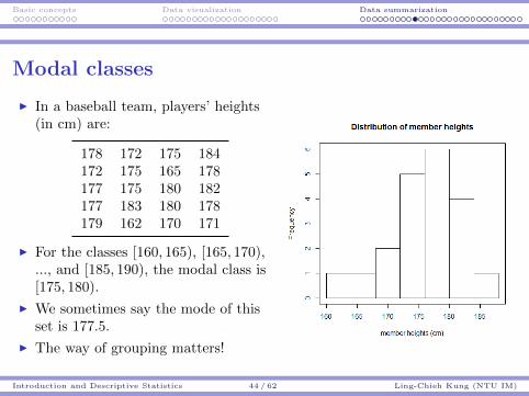
I In a baseball team, players’ heights(in cm) are:
178 172 175 184172 175 165 178177 175 180 182177 183 180 178179 162 170 171
I For the classes [160, 165), [165, 170),..., and [185, 190), the modal class is[175, 180).
I We sometimes say the mode of thisset is 177.5.
I The way of grouping matters!
Introduction and Descriptive Statistics 44 / 62 Ling-Chieh Kung (NTU IM)

Basic concepts Data visualization Data summarization
Variability
I Measures of variability describe the spread or dispersion of a setof data.
I Especially important when two sets of data have the same center.
Introduction and Descriptive Statistics 45 / 62 Ling-Chieh Kung (NTU IM)
Basic concepts Data visualization Data summarization
Ranges and Interquartile ranges
I The range of a set of data {xi}i=1,...,N is the difference between themaximum and minimum numbers, i.e.,
maxi=1,...,N
{xi} − mini=1,...,N
{xi}.
I The interquartile range of a set of data is the difference of the firstand third quartile.I It is the range of the middle 50 of data.I It excludes the effects of extreme values.
Introduction and Descriptive Statistics 46 / 62 Ling-Chieh Kung (NTU IM)

Basic concepts Data visualization Data summarization
Deviations from the mean
I Consider a set of population data{xi}i=1,...,N with mean µ.
I Intuitively, a way to measure thedispersion is to examine how each numberdeviates from the mean.
I For xi, the deviation from the populationmean is defined as
xi − µ.
I For a sample, the deviation from thesample mean of xi is
xi − x.
i xi deviation
1 1 1− 5 = −42 2 2− 5 = −33 4 4− 5 = −14 5 1− 5 = 05 6 6− 5 = 16 8 8− 5 = 37 9 9− 5 = 4
Mean 5
Introduction and Descriptive Statistics 47 / 62 Ling-Chieh Kung (NTU IM)

Basic concepts Data visualization Data summarization
Mean deviations
I May we summarize the N deviations intoa single number to summarize theaggregate deviation?
I Intuitively, we may sum them up and thencalculate the mean deviation:∑N
i=1(xi − µ)
N.
I Is it always 0?
i xi deviation
1 1 1− 5 = −42 2 2− 5 = −33 4 4− 5 = −14 5 1− 5 = 05 6 6− 5 = 16 8 8− 5 = 37 9 9− 5 = 4
Mean 5 0
Introduction and Descriptive Statistics 48 / 62 Ling-Chieh Kung (NTU IM)
Basic concepts Data visualization Data summarization
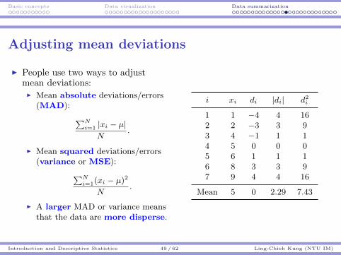
Adjusting mean deviations
I People use two ways to adjustmean deviations:I Mean absolute deviations/errors
(MAD): ∑Ni=1 |xi − µ|
N.
I Mean squared deviations/errors(variance or MSE):∑N
i=1(xi − µ)2
N.
I A larger MAD or variance meansthat the data are more disperse.
i xi di |di| d2i
1 1 −4 4 162 2 −3 3 93 4 −1 1 14 5 0 0 05 6 1 1 16 8 3 3 97 9 4 4 16
Mean 5 0 2.29 7.43
Introduction and Descriptive Statistics 49 / 62 Ling-Chieh Kung (NTU IM)
Basic concepts Data visualization Data summarization
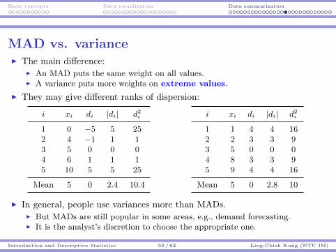
MAD vs. varianceI The main difference:
I An MAD puts the same weight on all values.I A variance puts more weights on extreme values.
I They may give different ranks of dispersion:
i xi di |di| d2i
1 0 −5 5 252 4 −1 1 13 5 0 0 04 6 1 1 15 10 5 5 25
Mean 5 0 2.4 10.4
i xi di |di| d2i
1 1 4 4 162 2 3 3 93 5 0 0 04 8 3 3 95 9 4 4 16
Mean 5 0 2.8 10
I In general, people use variances more than MADs.I But MADs are still popular in some areas, e.g., demand forecasting.I It is the analyst’s discretion to choose the appropriate one.
Introduction and Descriptive Statistics 50 / 62 Ling-Chieh Kung (NTU IM)

Basic concepts Data visualization Data summarization
Standard deviations
I One drawback of using variances is that the unit of measurement is thesquare of the original one.
I For the baseball team, the variance ofmember heights is 34.05 cm2. What is it?!
I People take the square root of a varianceto generate a standard deviation.
I The standard deviation of member heightsis √
34.05 ≈ 5.85 cm.
178 172 175 184172 175 165 178177 175 180 182177 183 180 178179 162 170 171
I A standard deviation typically has more managerial implications.
Introduction and Descriptive Statistics 51 / 62 Ling-Chieh Kung (NTU IM)
Basic concepts Data visualization Data summarization
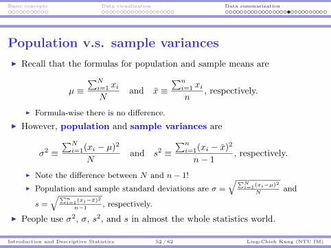
Population v.s. sample variances
I Recall that the formulas for population and sample means are
µ ≡∑N
i=1 xiN
and x ≡∑n
i=1 xin
, respectively.
I Formula-wise there is no difference.
I However, population and sample variances are
σ2 ≡∑N
i=1(xi − µ)2
Nand s2 ≡
∑ni=1(xi − x)2
n− 1, respectively.
I Note the difference between N and n− 1!
I Population and sample standard deviations are σ =
√∑Ni=1(xi−µ)2
Nand
s =
√∑ni=1(xi−x)2
n−1, respectively.
I People use σ2, σ, s2, and s in almost the whole statistics world.
Introduction and Descriptive Statistics 52 / 62 Ling-Chieh Kung (NTU IM)
Basic concepts Data visualization Data summarization
Coefficient of variation
I The coefficient of variation is the ratio of the standard deviation tothe mean:
Coefficient of variation =σ
µ.
I When will you use coefficients of variation?
Introduction and Descriptive Statistics 53 / 62 Ling-Chieh Kung (NTU IM)

Basic concepts Data visualization Data summarization
z-scores
I Consider a set of sample data {xi}i=1,...,n with sample mean x andsample standard deviation s. For xi, the z-score is
zi =xi − xs
.
I In a set of population data {xi}i=1,...,N with population mean µ andpopulation standard deviation σ, the z-score of xi is
zi =xi − µσ
.
I A value’s z-score measures for how many standard deviations itdeviates from the mean.
Introduction and Descriptive Statistics 54 / 62 Ling-Chieh Kung (NTU IM)
Basic concepts Data visualization Data summarization
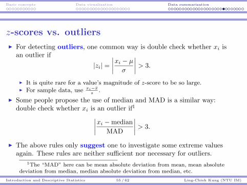
z-scores vs. outliers
I For detecting outliers, one common way is double check whether xi isan outlier if
|zi| =∣∣∣∣xi − µσ
∣∣∣∣ > 3.
I It is quite rare for a value’s magnitude of z-score to be so large.I For sample data, use xi−x
s.
I Some people propose the use of median and MAD is a similar way:double check whether xi is an outlier if1∣∣∣∣xi −median
MAD
∣∣∣∣ > 3.
I The above rules only suggest one to investigate some extreme valuesagain. These rules are neither sufficient nor necessary for outliers.
1The “MAD” here can be mean absolute deviation from mean, mean absolutedeviation from median, median absolute deviation from median, etc.
Introduction and Descriptive Statistics 55 / 62 Ling-Chieh Kung (NTU IM)

Basic concepts Data visualization Data summarization
CorrelationI Consider the size of a house and its price in a city:
Size Price(in m2) (in $1000)
75 31559 22985 35565 26172 23446 216107 30891 30675 28965 20488 26559 195
I How do we measure/describe the correlation (linear relationship)between the two variables?
Introduction and Descriptive Statistics 56 / 62 Ling-Chieh Kung (NTU IM)
Basic concepts Data visualization Data summarization
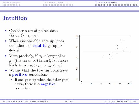
Intuition
I Consider a set of paired data{(xi, yi)}i=1,...,N .
I When one variable goes up, doesthe other one tend to go up ordown?
I More precisely, if xi is larger thanµx (the mean of the xis), is it morelikely to see yi > µy or yi < µy?
I We say that the two variables havea positive correlation.I If one goes up when the other goes
down, there is a negativecorrelation.
Introduction and Descriptive Statistics 57 / 62 Ling-Chieh Kung (NTU IM)

Basic concepts Data visualization Data summarization
Covariances
I We define the covariance of a set of two-dimensional (sample) data as
sxy ≡∑n
i=1(xi − x)(yi − y)
n− 1.
I If most points fall in the first and third quadrants, most(xi − µx)(y − µy) will be positive and sxy tends to be positive.
I Otherwise, sxy tends to be negative.
I So the covariance of house size and price is 617.16.
I Is it large or small?I This depends on how variable the two variables themselves are.
Introduction and Descriptive Statistics 58 / 62 Ling-Chieh Kung (NTU IM)

Basic concepts Data visualization Data summarization
Pearson’s correlation coefficientsI To take away the auto-variability of each variable itself, we define the
population and sample correlation coefficients as
r ≡ sxysxsy
,
I sx and sy are the sample standard deviations of xis and yis.I In our example, we have r = 617.16
16.78×50.45≈ 0.729.
I It can be shown that we always have −1 ≤ r ≤ 1.I r > 0: Positive correlation.I r = 0: No correlation.I r < 0: Negative correlation.
I People often determine the degree of correlation based on |s|:I 0 ≤ |s| < 0.25: A weak correlation.I 0.25 ≤ |s| < 0.5: A moderately weak correlation.I 0.5 ≤ |s| < 0.75: A moderately strong correlation.I 0.75 ≤ |s| ≤ 1: A strong correlation.
Introduction and Descriptive Statistics 59 / 62 Ling-Chieh Kung (NTU IM)

Basic concepts Data visualization Data summarization
Correlation vs. independence
I A correlation coefficient only measures how one variable linearlydepends on the other variable.
(r = 0.5973) (r = 0)
I Being uncorrelated does not mean being independent!
Introduction and Descriptive Statistics 60 / 62 Ling-Chieh Kung (NTU IM)

Basic concepts Data visualization Data summarization
Correlation vs. causationI A correlation coefficient only measures whether two variables correlate
with each other. High correlation does not mean causation.
I A causes B or B causes A? C causes A and B? Or just by chance?
Introduction and Descriptive Statistics 61 / 62 Ling-Chieh Kung (NTU IM)
Basic concepts Data visualization Data summarization
Correlation of qualitative variables
I Sometimes the variables are not quantitative/numeric.
I For ordinal data, we calculate their Spearman’s rank correlation.
I For nominal data, we calculate Cramer’s V.
Introduction and Descriptive Statistics 62 / 62 Ling-Chieh Kung (NTU IM)
Sampling Sampling distributions Hypothesis testing p-value, t test, and more
Statistics and Data Analysis for Engineers
Part 2:Hypothesis Testing and p-value
Ling-Chieh Kung
Department of Information ManagementNational Taiwan University
September 4, 2016
Hypothesis Testing and p-value 1 / 71 Ling-Chieh Kung (NTU IM)

Sampling Sampling distributions Hypothesis testing p-value, t test, and more
Road map
I Sampling.
I Sampling distributions.
I Hypothesis testing.
I p-value, t test, and more.
Hypothesis Testing and p-value 2 / 71 Ling-Chieh Kung (NTU IM)

Sampling Sampling distributions Hypothesis testing p-value, t test, and more
Random vs. nonrandom sampling
I Sampling is the process of selecting a subset of entities from the wholepopulation.
I Sampling can be random or nonrandom.
I If random, whether an entity is selected is probabilistic.I Randomly select 1000 phone numbers on the telephone book and then
call them.
I If nonrandom, it is deterministic.I Ask all your classmates for their preferences on iOS/Android.
I Most statistical methods are only for random sampling.
I Some popular random sampling techniques:I Simple random sampling.I Stratified random sampling.I Cluster (or area) random sampling.
Hypothesis Testing and p-value 3 / 71 Ling-Chieh Kung (NTU IM)

Sampling Sampling distributions Hypothesis testing p-value, t test, and more
Simple random sampling
I In simple random sampling, each entity has the same probability ofbeing selected.
I The good part of simple random sampling is simple.
I However, it may result in nonrepresentative samples.
I In simple random sampling, there are some possibilities that toomuch data we sample fall in the same stratum.I They have the same property.I E.g., it is possible that all randomly sampled voters are younger than 40.I The sample is thus nonrepresentative.
I How to fix this problem?
Hypothesis Testing and p-value 4 / 71 Ling-Chieh Kung (NTU IM)
Sampling Sampling distributions Hypothesis testing p-value, t test, and more
Stratified random sampling
I We may apply stratified random sampling.
I We first split the whole population into several strata.I Data in one stratum should be (relatively) homogeneous.I Data in different strata should be (relatively) heterogeneous.
I We then use simple random sampling for each stratum.
Hypothesis Testing and p-value 5 / 71 Ling-Chieh Kung (NTU IM)
Sampling Sampling distributions Hypothesis testing p-value, t test, and more
Stratified random sampling
I As an example, suppose that we want to sample 40 out of 1000graduates to understand the number of credits they get at school.
I Suppose that 100 students double majored, then we can split the wholepopulation into two strata:
Stratum Strata size
Double major 100No double major 900
I To sample 40 graduates, we sample 40× 1001000 = 4 from the
double-major stratum and 36 from the other stratum.
Hypothesis Testing and p-value 6 / 71 Ling-Chieh Kung (NTU IM)
Sampling Sampling distributions Hypothesis testing p-value, t test, and more
Stratified random sampling
I We may further split the population into more strata.I Double major: Yes or no.I Class: 1994-1998, 1999-2003, 2004-2008, or 2009-2012.I This stratification makes sense only if students in different classes tend
to take different numbers of units.
I Stratified random sampling is good in reducing sample error.
I But it can be hard to identify a reasonable stratification.
I It is also more costly and time-consuming.
Hypothesis Testing and p-value 7 / 71 Ling-Chieh Kung (NTU IM)

Sampling Sampling distributions Hypothesis testing p-value, t test, and more
Cluster (or area) random sampling
I Imagine that you are going to introduce a new product into all theretail stores in Taiwan.
I If the product is actually unpopular, an introduction with a largequantity will incur a huge lost.
I How to get an idea about the popularity?
I Typically we first try to introduce the product in a small area. Weput the product on the shelves only in those stores in the specified area.
I This is the idea of cluster (or area) random sampling.I Those consumers in the area form a sample.
Hypothesis Testing and p-value 8 / 71 Ling-Chieh Kung (NTU IM)
Sampling Sampling distributions Hypothesis testing p-value, t test, and more
Cluster (or area) random sampling
I In cluster random sampling, we define clusters.
I We will only choose one or some clusters and then collect all thedata in these clusters.I If a cluster is too large, we may further split it into multiple
second-stage clusters.
I Therefore, we want data in a cluster to be heterogeneous, and dataacross clusters somewhat homogeneous.
I For example, people may do cluster random sampling to understandthe popularity of a new product. Those chosen cities (counties, states,etc.) are called test market cities (counties, states, etc.).I People use cluster random sampling in this case because of its feasibility
and convenience.I We should select test market cities whose population profiles are similar
to that of the entire country.
Hypothesis Testing and p-value 9 / 71 Ling-Chieh Kung (NTU IM)

Sampling Sampling distributions Hypothesis testing p-value, t test, and more
Nonrandom sampling
I Sometimes we do nonrandom sampling.
I Convenience sampling.I The researcher sample data that are easy to sample.
I Judgment sampling.I The researcher decides who to ask or what data to collect.
I Quota sampling.I In each stratum, we use whatever method that is easy to fill the quota, a
predetermined number of samples in the stratum.
I Snowball sampling.I Once we ask one person, we ask her/him to suggest others.
I Nonrandom sampling cannot be analyzed by the statistical methodswe introduce in this course.
Hypothesis Testing and p-value 10 / 71 Ling-Chieh Kung (NTU IM)

Sampling Sampling distributions Hypothesis testing p-value, t test, and more
Road map
I Sampling.
I Sampling distributions.
I Hypothesis testing.
I p-value, t test, and more. .
Hypothesis Testing and p-value 11 / 71 Ling-Chieh Kung (NTU IM)
Sampling Sampling distributions Hypothesis testing p-value, t test, and more
Sampling distributions
I When we cannot examine the whole population, we study a sample.I What will be contained in a random sample is unpredictable.I We need to know the probability distribution of a sample so that we
may connect the sample with the population.
I The probability distribution of a sample is a sampling distribution.
Hypothesis Testing and p-value 12 / 71 Ling-Chieh Kung (NTU IM)

Sampling Sampling distributions Hypothesis testing p-value, t test, and more
Sampling distributionsI A factory produces bags of candies. Ideally, each bag should weigh 2
kg. As the production process cannot be perfect, a bag of candiesshould weigh between 1.8 and 2.2 kg.
I Let X be the weight of a bag of candies. Let µ and σ be its expectedvalue and standard deviation.I Is µ = 2?I Is 1.8 < µ < 2.2?I How large is σ?
I Let’s sample:I In a random sample of 1 bag of candies, suppose it weighs 2.1 kg. May
we conclude that 1.8 < µ < 2.2?I What if the average weight of 5 bags in a random sample is 2.1 kg?I What if the sample size is 10, 50, or 100?I What if the mean is 2.3 kg?
I We need to know the sampling distribution of those statistics (samplemean, sample standard deviation, etc.).
Hypothesis Testing and p-value 13 / 71 Ling-Chieh Kung (NTU IM)

Sampling Sampling distributions Hypothesis testing p-value, t test, and more
Sample means
I The sample mean is one of the most important statistics.
Definition 1
Let {Xi}i=1,...,n be a sample from a population, then
x =
∑ni=1Xi
n
is the sample mean.
I Sometimes we write xn to emphasize that the sample size is n.
I We assume that Xi and Xj are independent for all i 6= j.I This is fine if n� N , i.e., we sample a few items from a large population.I In practice, we require n ≤ 0.05N .
Hypothesis Testing and p-value 14 / 71 Ling-Chieh Kung (NTU IM)

Sampling Sampling distributions Hypothesis testing p-value, t test, and more
Means and variances of sample meansI Suppose the population mean and variance are µ and σ2, respectively.
I These two numbers are fixed.
I A sample mean x is a random variable.I It has its expected value E[x], variance Var(x), and standard deviation√
Var(x). These numbers are all fixedI They are also denoted as µx, σ2
x, and σx, respectively.
I For any population, we have the following theorem:
Proposition 1 (Mean and variance of a sample mean)
Let {Xi}i=1,...,n be a size-n random sample from a population withmean µ and variance σ2, then we have
µx = µ, σ2x =
σ2
n, and σx =
σ√n.
Hypothesis Testing and p-value 15 / 71 Ling-Chieh Kung (NTU IM)
Sampling Sampling distributions Hypothesis testing p-value, t test, and more
Means and variances of sample means
I Do the terms confuse you?I The sample mean vs. the mean of the sample mean.I The sample variance vs. the variance of the sample mean.
I By definition, they are:I x = 1
n
∑ni=1 Xi; a random variable.
I E[x]; a constant.
I s2 = 1n−1
∑ni=1(Xi − x)2; a random variable.
I Var(x); a constant.
I The sample variance also has its mean and variance.
Hypothesis Testing and p-value 16 / 71 Ling-Chieh Kung (NTU IM)

Sampling Sampling distributions Hypothesis testing p-value, t test, and more
Example: Quality inspection
I The weight of a bag of candies follow a normal distribution with meanµ = 2 and standard deviation σ = 0.2.
I Suppose the quality control officer decides to sample 4 bags andcalculate the sample mean x. She will punish me if x /∈ [1.8, 2.2].I Note that my production process is actually “good:” µ = 2.I Unfortunately, it is not perfect: σ > 0.I We may still be punished (if we are unlucky) even though µ = 2.
I What is the probability that I will be punished?I We want to calculate 1− Pr(1.8 < x < 2.2).I We know that µx = µ = 2 and σx = σ√
4= 0.1.
I But we do not know the probability distribution of x!
Hypothesis Testing and p-value 17 / 71 Ling-Chieh Kung (NTU IM)

Sampling Sampling distributions Hypothesis testing p-value, t test, and more
Sampling from a normal population
I If the population is normal, the sample mean is also normal!
Proposition 2
Let {Xi}i=1,...,n be a size-n random sample from a normal populationwith mean µ and standard deviation σ. Then
x ∼ ND
(µ,
σ√n
).
I We already know that µx = µ and σx = σ√n
. This is true regardless of
the population distribution.
I When the population is normal, the sample mean will also be normal.
Hypothesis Testing and p-value 18 / 71 Ling-Chieh Kung (NTU IM)

Sampling Sampling distributions Hypothesis testing p-value, t test, and more
Example revisited: Quality inspection
I The weight of a bag of candies follow a normal distribution with meanµ = 2 and standard deviation σ = 0.2.
I Suppose the quality control officer decides to sample 4 bags andcalculate the sample mean x. She will punish me if x /∈ [1.8, 2.2].
I What is the probability that I will be punished?I The distribution of the sample mean x is ND(2, 0.1).I Pr(x < 1.8) + Pr(x > 2.2) ≈ 0.045.
Hypothesis Testing and p-value 19 / 71 Ling-Chieh Kung (NTU IM)
Sampling Sampling distributions Hypothesis testing p-value, t test, and more
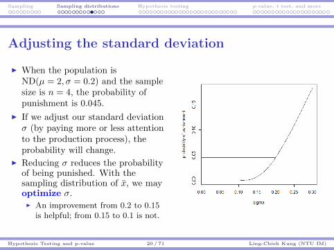
Adjusting the standard deviation
I When the population isND(µ = 2, σ = 0.2) and the samplesize is n = 4, the probability ofpunishment is 0.045.
I If we adjust our standard deviationσ (by paying more or less attentionto the production process), theprobability will change.
I Reducing σ reduces the probabilityof being punished. With thesampling distribution of x, we mayoptimize σ.I An improvement from 0.2 to 0.15
is helpful; from 0.15 to 0.1 is not.
Hypothesis Testing and p-value 20 / 71 Ling-Chieh Kung (NTU IM)

Sampling Sampling distributions Hypothesis testing p-value, t test, and more
Adjusting the sample size
I When the population is ND(2, 0.2)and the sample size is n = 4, theprobability of punishment is 0.045.
I If the quality control officerincreases the sample size n, theprobability will decrease.
I µ = 2 is actually ideal. A largersample size makes the officer lesslikely to make a mistake.
Hypothesis Testing and p-value 21 / 71 Ling-Chieh Kung (NTU IM)
Sampling Sampling distributions Hypothesis testing p-value, t test, and more
Distribution of the sample mean
I So now we have one general conclusion: When we sample from anormal population, the sample mean is also normal.I And its mean and standard deviation are µ and σ√
n, respectively.
I What if the population is non-normal?
I Fortunately, we have a very powerful theorem, the central limittheorem, which applies to any population.
Hypothesis Testing and p-value 22 / 71 Ling-Chieh Kung (NTU IM)

Sampling Sampling distributions Hypothesis testing p-value, t test, and more
Central limit theorem
I The theorem says that a sample mean is approximately normalwhen the sample size is large enough.
Proposition 3 (Central limit theorem)
Let {Xi}i=1,...,n be a size-n random sample from a population withmean µ and standard deviation σ. Let xn be the sample mean. Ifσ <∞, then xn converges to ND(µ, σ√
n) as n→∞.
I How large is “large enough”?
I In practice, typically n ≥ 30 is believed to be large enough.
Hypothesis Testing and p-value 23 / 71 Ling-Chieh Kung (NTU IM)
Sampling Sampling distributions Hypothesis testing p-value, t test, and more
Road map
I Sampling.
I Sampling distributions.
I Hypothesis testing.
I p-value, t test, and more. .
Hypothesis Testing and p-value 24 / 71 Ling-Chieh Kung (NTU IM)
Sampling Sampling distributions Hypothesis testing p-value, t test, and more
Hypothesis testing
I How do scientists (physicists, chemists, etc.) do research?I Observe phenomena.I Make hypotheses.I Test the hypotheses through experiments (or other methods).I Make conclusions about the hypotheses.
I Social scientists and business researchers do the same thing withhypothesis testing.I One of the most important technique of statistical inference.I A technique for (statistically) proving things.I Relying on sampling distributions.
Hypothesis Testing and p-value 25 / 71 Ling-Chieh Kung (NTU IM)

Sampling Sampling distributions Hypothesis testing p-value, t test, and more
People ask questions
I In the business (or social science) world, people ask questions:I Are older workers more loyal to a company?I Does the newly hired CEO enhance our profitability?I Is one candidate preferred by more than 50% voters?I Do teenagers eat fast food more often than adults?I Is the quality of our products stable enough?
I How should we answer these questions?
I Statisticians suggest:I First make a hypothesis.I Then test it with samples and statistical methods.
Hypothesis Testing and p-value 26 / 71 Ling-Chieh Kung (NTU IM)

Sampling Sampling distributions Hypothesis testing p-value, t test, and more
Statistical hypotheses
I A statistical hypothesis is a formal way of stating a hypothesis.I Typically it is a mathematical description of parameters to test.
I It contains two parts:I The null hypothesis (denoted as H0).I The alternative hypothesis (denoted as Ha or H1).
I The alternative hypothesis is:I The thing that we want (need) to prove.I The conclusion that can be made only if we have a strong evidence.
I The null hypothesis corresponds to a default position.I We first assume that the null hypothesis is correct.I Then we collect sample data.I If under the null hypothesis it is quite unlikely to see our observed
result, we claim that the null hypothesis is wrong.
Hypothesis Testing and p-value 27 / 71 Ling-Chieh Kung (NTU IM)
Sampling Sampling distributions Hypothesis testing p-value, t test, and more
Statistical hypotheses: example 1
I In our factory, we produce packs of candy whose average weight shouldbe 1 kg.
I One day, a consumer told us that his pack only weighs 900 g.
I We need to know whether this is just a rare event or our productionsystem is out of control.
I If (we believe) the system is out of control, we need to shutdown themachine and spend two days for inspection and maintenance. This willcost us at least $100,000.
I So we should not to believe that our system is out of control justbecause of one complaint. What should we do?
Hypothesis Testing and p-value 28 / 71 Ling-Chieh Kung (NTU IM)

Sampling Sampling distributions Hypothesis testing p-value, t test, and more
Statistical hypotheses: example 1
I We first state a hypothesis: “Our production system is under control.”
I Then we ask: Is there a strong enough evidence showing that thehypothesis is wrong, i.e., the system is out of control?I Initially, we assume that our system is under control.I Then we do a survey to see if we have a strong enough evidence.I We shutdown machines only if we can “prove” that the system is indeed
out of control.
I Let µ be the average weight, the statistical hypothesis is
H0 : µ = 1
Ha : µ 6= 1.
Hypothesis Testing and p-value 29 / 71 Ling-Chieh Kung (NTU IM)

Sampling Sampling distributions Hypothesis testing p-value, t test, and more
Statistical hypotheses: example 2
I In our society, we adopt the presumption of innocence.I One is considered innocent until proven guilty.
I So when there is a person who probably stole some money:
H0 : The person is innocent
Ha : The person is guilty.
I There are two possible errors:I One is guilty but we think she/he is innocent.I One is innocent but we think she/he is guilty.
I Which one is more critical?I It is unacceptable that an innocent person is considered guilty.I We will say one is guilty only if there is a strong evidence.
Hypothesis Testing and p-value 30 / 71 Ling-Chieh Kung (NTU IM)
Sampling Sampling distributions Hypothesis testing p-value, t test, and more
Statistical hypotheses: example 3
I Consider the following hypothesis: “The candidate is preferred by morethan 50% voters.”
I As we need a default position, and the percentage that we care aboutis 50%, we will choose our null hypothesis as
H0 : p = 0.5.
I p is the population proportion of voters preferring the candidate.I More precisely, let Xi = 1 if voter i prefers this candidate and 0
otherwise, i = 1, ..., N , then p =∑N
i=1Xi
N.
I How about the alternative hypothesis? Should it be
Ha : p > 0.5 or Ha : p < 0.5?
Hypothesis Testing and p-value 31 / 71 Ling-Chieh Kung (NTU IM)

Sampling Sampling distributions Hypothesis testing p-value, t test, and more
Statistical hypotheses: example 3
I The choice of the alternative hypothesis depends on the relateddecisions or actions to make.
I Suppose one will go for the election only if she thinks she will win (i.e.,p > 0.5), the alternative hypothesis will be
Ha : p > 0.5.
I Suppose one tends to participate in the election and will give up only ifthe chance is slim, the alternative hypothesis will be
Ha : p < 0.5.
I The alternative hypothesis is “the thing we want (need) to prove.”
Hypothesis Testing and p-value 32 / 71 Ling-Chieh Kung (NTU IM)
Sampling Sampling distributions Hypothesis testing p-value, t test, and more
Two types of errors
I Type-1 error (false positive): Rejecting a true null hypothesis.I There is nothing, but we say there is one.
I Type-2 error (false negative): Do not reject a false null hypothesis.I There is something, but we do not see it.
Hypothesis Testing and p-value 33 / 71 Ling-Chieh Kung (NTU IM)

Sampling Sampling distributions Hypothesis testing p-value, t test, and more
Hypothesis Testing and p-value 34 / 71 Ling-Chieh Kung (NTU IM)

Sampling Sampling distributions Hypothesis testing p-value, t test, and more
Remarks
I We want to control the chances for us to make these mistakes.I Unfortunately, we cannot control both.I We choose to control the probability of a type-1 error.I The choice of the default position is important.
I For setting up a statistical hypothesis:I Our default position will be put in the null hypothesis.I The thing we want to prove (i.e., the thing that needs a strong evidence)
will be put in the alternative hypothesis.
I For writing the mathematical statement:I The equal sign (=) will always be put in the null hypothesis.I The alternative hypothesis contains an unequal sign or strict
inequality: 6=, >, or <.
I The direction of the alternative hypothesis, when it is an inequality,depends on the context.
Hypothesis Testing and p-value 35 / 71 Ling-Chieh Kung (NTU IM)

Sampling Sampling distributions Hypothesis testing p-value, t test, and more
One-tailed tests and two-tailed tests
I If the alternative hypothesis contains an unequal sign (6=), the test is atwo-tailed test.
I If it contains a strict inequality (> or <), the test is a one-tailed test.
I Suppose we want to test the value of the population mean.I In a two-tailed test, we test whether the population mean significantly
deviates from a hypothesized value. We do not care whether it is largerthan or smaller than.
I In a one-tailed test, we test whether the population mean significantlydeviates from a hypothesized value in a specific direction.
Hypothesis Testing and p-value 36 / 71 Ling-Chieh Kung (NTU IM)
Sampling Sampling distributions Hypothesis testing p-value, t test, and more
The first example: a two-tailed test
I Let’s test the average weight (in g) of our products.
H0 : µ = 1000
Ha : µ 6= 1000.
I The variance of the product weights is σ2 = 40000 g2.I The case with unknown σ2 will be discussed later.
I A random sample has been collected.I Suppose the sample size n = 100.I Suppose the sample mean X = 963.
I How to make a conclusion?
Hypothesis Testing and p-value 37 / 71 Ling-Chieh Kung (NTU IM)
Sampling Sampling distributions Hypothesis testing p-value, t test, and more
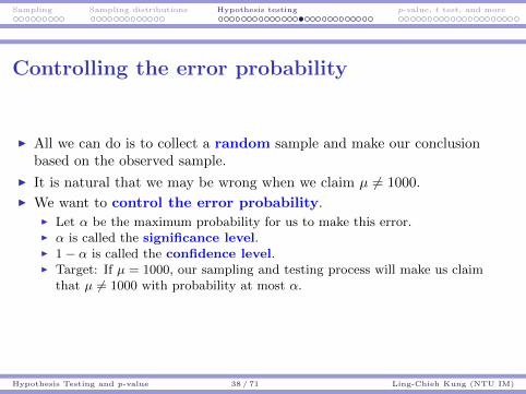
Controlling the error probability
I All we can do is to collect a random sample and make our conclusionbased on the observed sample.
I It is natural that we may be wrong when we claim µ 6= 1000.
I We want to control the error probability.I Let α be the maximum probability for us to make this error.I α is called the significance level.I 1− α is called the confidence level.I Target: If µ = 1000, our sampling and testing process will make us claim
that µ 6= 1000 with probability at most α.
Hypothesis Testing and p-value 38 / 71 Ling-Chieh Kung (NTU IM)

Sampling Sampling distributions Hypothesis testing p-value, t test, and more
Rejection rule
I Now let’s test with the significance level α = 0.05.
I Intuitively, if X deviates from 1000 a lot, we should reject the nullhypothesis and believe that µ 6= 1000.I If µ = 1000, it is so unlikely to observe such a large deviation.I So such a large deviation provides a strong evidence.
I So we start by sampling and calculating the sample mean.
I We want to construct a rejection rule: If |X − 1000| > d, we rejectH0. We need to calculate d.
Hypothesis Testing and p-value 39 / 71 Ling-Chieh Kung (NTU IM)
Sampling Sampling distributions Hypothesis testing p-value, t test, and more
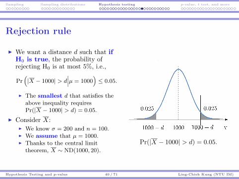
Rejection rule
I We want a distance d such that ifH0 is true, the probability ofrejecting H0 is at most 5%, i.e.,
Pr(|X − 1000| > d
∣∣∣µ = 1000)≤ 0.05.
I The smallest d that satisfies theabove inequality requiresPr(|X − 1000| > d) = 0.05.
I Consider X:I We know σ = 200 and n = 100.I We assume that µ = 1000.I Thanks to the central limit
theorem, X ∼ ND(1000, 20).
Pr(|X − 1000| > d) = 0.05.
Hypothesis Testing and p-value 40 / 71 Ling-Chieh Kung (NTU IM)
Sampling Sampling distributions Hypothesis testing p-value, t test, and more
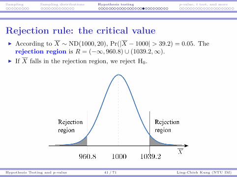
Rejection rule: the critical valueI According to X ∼ ND(1000, 20), Pr(|X − 1000| > 39.2) = 0.05. The
rejection region is R = (−∞, 960.8) ∪ (1039.2,∞).
I If X falls in the rejection region, we reject H0.
Hypothesis Testing and p-value 41 / 71 Ling-Chieh Kung (NTU IM)

Sampling Sampling distributions Hypothesis testing p-value, t test, and more
Rejection rule: the critical value
I Because x = 963 /∈ R, we cannot reject H0.I The deviation from 1000 is not large enough.I The evidence is not strong enough.
Hypothesis Testing and p-value 42 / 71 Ling-Chieh Kung (NTU IM)

Sampling Sampling distributions Hypothesis testing p-value, t test, and more
Rejection rule: the critical value
I In this example, the two values 960.8 and 1039.2 are the criticalvalues for rejection.I If the sample mean is more extreme than one of the critical values, we
reject H0.I Otherwise, we do not reject H0.
I x = 963 is not strong enough to support Ha: µ 6= 1000.
I Concluding statement:I Because the sample mean does not lie in the rejection region, we cannot
reject H0.I With a 95% confidence level, there is no strong evidence showing that
the average weight is not 1000 g.I Therefore, we should not shutdown machines to do an inspection.
Hypothesis Testing and p-value 43 / 71 Ling-Chieh Kung (NTU IM)
Sampling Sampling distributions Hypothesis testing p-value, t test, and more
Summary
I We want to know whether the machine is out of control.I If the machine is actually good, we do not want to reach a conclusion
that requires an inspection and maintenance.I We will do the inspection only if we have a strong evidence suggesting
that µ 6= 1000.
I We want to know whether H0 is false, i.e., µ 6= 1000.
I We control the probability of making a wrong conclusion.I We should not reject H0 if it is true.I We limit the probability at α = 5%.
I We will conclude that H0 is false if X falls in the rejection region.I The calculation of the the critical values is based on the normal
distribution, which can always be transformed to the z distribution.I This is called a z test.
Hypothesis Testing and p-value 44 / 71 Ling-Chieh Kung (NTU IM)

Sampling Sampling distributions Hypothesis testing p-value, t test, and more
Not rejecting vs. accepting
I We should be careful in writing our conclusions:I Wrong: Because the sample mean does not lie in the rejection region,
we accept H0. With a 95% confidence level, there is a strong evidenceshowing that the average weight is 1000 g.
I Right: Because the sample mean does not lie in the rejection region, wecannot reject H0. With a 95% confidence level, there is no strongevidence showing that the average weight is not 1000 g.
I Unable to prove one thing is false does not mean it is true!
Hypothesis Testing and p-value 45 / 71 Ling-Chieh Kung (NTU IM)
Sampling Sampling distributions Hypothesis testing p-value, t test, and more
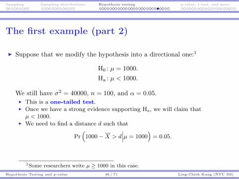
The first example (part 2)
I Suppose that we modify the hypothesis into a directional one:1
H0 : µ = 1000.
Ha : µ < 1000.
We still have σ2 = 40000, n = 100, and α = 0.05.I This is a one-tailed test.I Once we have a strong evidence supporting Ha, we will claim thatµ < 1000.
I We need to find a distance d such that
Pr(
1000−X > d∣∣∣µ = 1000
)= 0.05.
1Some researchers write µ ≥ 1000 in this case.
Hypothesis Testing and p-value 46 / 71 Ling-Chieh Kung (NTU IM)
Sampling Sampling distributions Hypothesis testing p-value, t test, and more
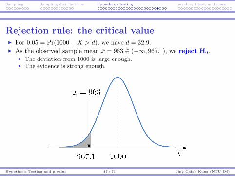
Rejection rule: the critical valueI For 0.05 = Pr(1000−X > d), we have d = 32.9.I As the observed sample mean x = 963 ∈ (−∞, 967.1), we reject H0.
I The deviation from 1000 is large enough.I The evidence is strong enough.
Hypothesis Testing and p-value 47 / 71 Ling-Chieh Kung (NTU IM)

Sampling Sampling distributions Hypothesis testing p-value, t test, and more
Rejection rule: the critical value
I In this example, 967.1 is the critical values for rejection.I If the sample mean is more extreme than (in this case, below) the critical
value, we reject H0.I Otherwise, we do not reject H0.
I There is a strong evidence supporting Ha: µ < 1000.
I Concluding statement:I Because the sample mean lies in the rejection region, we reject H0.
With a 95% confidence level, there is a strong evidence showing that theaverage weight is less than 1000 g.
Hypothesis Testing and p-value 48 / 71 Ling-Chieh Kung (NTU IM)

Sampling Sampling distributions Hypothesis testing p-value, t test, and more
One-tailed tests vs. two-tailed testsI When should we use a two-tailed test?
I We use a two-tailed test when we are lack of the direction information.I E.g., we suspect that the population mean has changed, but we have
no idea about whether it becomes larger or smaller.
I If we know or believe that the change is possible only in onedirection, we may use a one-tailed test.
I Having more information (i.e., knowing the direction of change) makesrejection “easier,”, i.e., easier to find a strong enough evidence.
Hypothesis Testing and p-value 49 / 71 Ling-Chieh Kung (NTU IM)

Sampling Sampling distributions Hypothesis testing p-value, t test, and more
Summary
I Distinguish the following pairs:I One- and two-tailed tests.I No evidence showing H0 is false and having evidence showing H0 is true.I Not rejecting H0 and accepting H0.I Using = and using ≥ or ≤ in the null hypothesis.
Hypothesis Testing and p-value 50 / 71 Ling-Chieh Kung (NTU IM)
Sampling Sampling distributions Hypothesis testing p-value, t test, and more
Road map
I Sampling.
I Sampling distributions.
I Hypothesis testing.
I p-value, t test, and more. .
Hypothesis Testing and p-value 51 / 71 Ling-Chieh Kung (NTU IM)

Sampling Sampling distributions Hypothesis testing p-value, t test, and more
The p-value
I The p-value is an important, meaningful, and widely-adopted tool forhypothesis testing.
Definition 2
For an observed value of a statistic in a statistical test, the p-value isthe probability of observing a value that is more extreme than theobserved value under the assumption that the null hypothesis is true.
I Calculated based on an observed value of the statistic.I Is the tail probability of the observed value.I Assuming that the null hypothesis is true.
Hypothesis Testing and p-value 52 / 71 Ling-Chieh Kung (NTU IM)
Sampling Sampling distributions Hypothesis testing p-value, t test, and more
The p-value
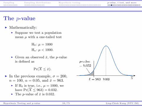
I Mathematically:I Suppose we test a population
mean µ with a one-tailed test
H0 : µ = 1000
Ha : µ < 1000.
I Given an observed x, the p-valueis defined as
Pr(X ≤ x).
I In the previous example, σ = 200,n = 100, α = 0.05, and x = 963.I If H0 is true, i.e., µ = 1000, we
have Pr(X ≤ 963) = 0.032.I The p-value of x is 0.032.
Hypothesis Testing and p-value 53 / 71 Ling-Chieh Kung (NTU IM)

Sampling Sampling distributions Hypothesis testing p-value, t test, and more
How to use the p-value?
I The p-value can be used for constructing a rejection rule.
I For a one-tailed test:I If the p-value is smaller than α, we reject H0.I If the p-value is greater than α, we do not reject H0.
I In our example, the one-tailed test is
H0 : µ = 1000
Ha : µ < 1000.
I We have α = 0.05.I Because the p-value 0.032 < 0.05, we reject H0.
Hypothesis Testing and p-value 54 / 71 Ling-Chieh Kung (NTU IM)
Sampling Sampling distributions Hypothesis testing p-value, t test, and more
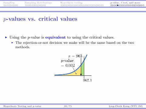
p-values vs. critical values
I Using the p-value is equivalent to using the critical values.I The rejection-or-not decision we make will be the same based on the two
methods.
Hypothesis Testing and p-value 55 / 71 Ling-Chieh Kung (NTU IM)
Sampling Sampling distributions Hypothesis testing p-value, t test, and more
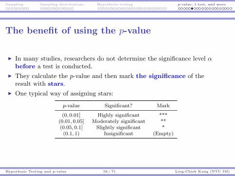
The benefit of using the p-value
I In many studies, researchers do not determine the significance level αbefore a test is conducted.
I They calculate the p-value and then mark the significance of theresult with stars.
I One typical way of assigning stars:
p-value Significant? Mark
(0, 0.01] Highly significant ***(0.01, 0.05] Moderately significant **(0.05, 0.1] Slightly significant *
(0.1, 1) Insignificant (Empty)
Hypothesis Testing and p-value 56 / 71 Ling-Chieh Kung (NTU IM)

Sampling Sampling distributions Hypothesis testing p-value, t test, and more
The size of a p-value
I Suppose one is testing whether people at different ages sleep for atleast eight hours per day in average.I Age groups: [10, 15), [15, 20), [20, 35), etc.I For group i, a one-tailed test is conducted. Ha : µi > 8.I The result may be presented in a table:
Group Age group p-value
1 [10,15) 0.0002***2 [15,20) 0.23 [20,25) 0.06*4 [25,30) 0.04**5 [30,35) 0.03**
I A smaller p-value does NOT mean a larger deviation!I We cannot conclude that µ5 > µ4, µ1 > µ3, etc.I There are other tests for the difference between two population means.
Hypothesis Testing and p-value 57 / 71 Ling-Chieh Kung (NTU IM)

Sampling Sampling distributions Hypothesis testing p-value, t test, and more
The p-value for two-tailed tests
I How to construct the rejection rule for a two-tailed test?I If the p-value is smaller than α
2, we reject H0.
I If the p-value is greater than α2
, we do not reject H0.
I Consider the two-tailed test
H0 : µ = 1000.
Ha : µ 6= 1000.
I We have α = 0.05.I Because the p-value 0.032 > α
2= 0.025, we do not reject H0.
I Some researchers/books/software use another definition:I The p-value for a two-tailed test is two times of that for the
corresponding one-tailed test.I They then compare this p-value with α.
Hypothesis Testing and p-value 58 / 71 Ling-Chieh Kung (NTU IM)

Sampling Sampling distributions Hypothesis testing p-value, t test, and more
Summary
I The p-value is the tail probability of the realized value of a statisticsassuming the null hypothesis is true.
I The p-value method is an alternative way of forming the rejection rule.I It is equivalent to the critical-value method.
I The p-value is related to the probability for H0 to be false.
I It does not measure the magnitude of the deviation.
Hypothesis Testing and p-value 59 / 71 Ling-Chieh Kung (NTU IM)

Sampling Sampling distributions Hypothesis testing p-value, t test, and more
The z test
I In example 1, basically we use the fact that X ∼ ND(µ, σ√n
.
I This implies that X−µσ/√n∼ ND(0, 1), the so-called standard normal
distribution, or the z distribution.I Therefore, this test is called the z test.
I This requires the knowledge about σ.
Hypothesis Testing and p-value 60 / 71 Ling-Chieh Kung (NTU IM)

Sampling Sampling distributions Hypothesis testing p-value, t test, and more
When the variance is unknown
I When the population variance σ2 is unknown, the quantity X−µσ/√n
is
unknown.
I What if we use the sample variance S2 as a substitute?
Proposition 4
For a normal population, the quantity
T =X − µS/√n
follows the t distribution with degree of freedom n− 1.
I What is the t distribution?
Hypothesis Testing and p-value 61 / 71 Ling-Chieh Kung (NTU IM)

Sampling Sampling distributions Hypothesis testing p-value, t test, and more
The t distribution
I The t distribution is defined as follows:
Definition 3
A random variable X follows the t distribution with degree of freedomn, denoted as X ∼ t(n), if
f(x|n) =Γ(n+1
2 )√nπΓ(n2 )
(1 +
x2
n
)−n+12
,
for all x ∈ (−∞,∞).
I Γ(x) =
∫ ∞0
zx−1e−zdz is the gamma function.
Hypothesis Testing and p-value 62 / 71 Ling-Chieh Kung (NTU IM)

Sampling Sampling distributions Hypothesis testing p-value, t test, and more
The z and t distributions
I Let’s compare Z = X−µσ/√n
and T = X−µS/√n
.
I Because we do not know σ, we use S to substitute it.I Z ∼ ND(0, 1) and T ∼ t(n− 1).I As the t distribution is a substitution of the z distribution, it is designed
to be also centered at 0: E[T ] = E[Z] = 0.I However, as we add one more random variable into the formula (σ is a
known constant), T will be “more random” than Z, i.e.,Var(T ) > Var(Z).
I Graphically, t curves will be flatter than the z curve.I Fact: t(n)→ ND(0, 1) as n→∞.
Hypothesis Testing and p-value 63 / 71 Ling-Chieh Kung (NTU IM)

Sampling Sampling distributions Hypothesis testing p-value, t test, and more
Hypothesis Testing and p-value 64 / 71 Ling-Chieh Kung (NTU IM)

Sampling Sampling distributions Hypothesis testing p-value, t test, and more
The t test
I We will use the t test to test the population mean if the population isnormal.
I If the sample size is large, we may still use the z distribution with ssubstituting σ.
Hypothesis Testing and p-value 65 / 71 Ling-Chieh Kung (NTU IM)
Sampling Sampling distributions Hypothesis testing p-value, t test, and more
Example 2
I An MBA program seldom admits applicants without a work experiencelonger than two years.
I To test whether the average work year of admitted students is abovetwo years, 20 admitted applicants are randomly selected.
I Their work experiences prior to entering the program are recorded.I Prior to entering the program, they have an average work experience of
2.5 years. This is the sample mean.I The sample standard deviation is 1.3765 years.
I The population is believed to be normal.
I The confidence level is set to 95%.
Hypothesis Testing and p-value 66 / 71 Ling-Chieh Kung (NTU IM)
Sampling Sampling distributions Hypothesis testing p-value, t test, and more
Example 2: hypothesis
I Suppose the one asking the question is a potential applicant with oneyear of work experience. He is pessimistic and will apply for theprogram only if the average work experience is proven to be less thantwo years.
I The hypothesis is
H0 : µ = 2
Ha : µ < 2.
I µ is the average work experience (in years) of all admitted applicantsprior to entering the program.
I To encourage him, we need to give him a strong evidence showing thathis chance is high.
Hypothesis Testing and p-value 67 / 71 Ling-Chieh Kung (NTU IM)

Sampling Sampling distributions Hypothesis testing p-value, t test, and more
Example 2: hypothesis and test
I Suppose he is optimistic and will not apply for the program only ifthe average work experience is proven to be greater than two.
I The hypothesis becomes
H0 : µ = 2
Ha : µ > 2.
I To discourage him, we need to give him a strong evidence showing thathis chance is slim.
I Let’s consider the optimistic candidate (and Ha : µ > 2) first.
I Because the population variance is unknown and the population isnormal, we may use the t test.
Hypothesis Testing and p-value 68 / 71 Ling-Chieh Kung (NTU IM)

Sampling Sampling distributions Hypothesis testing p-value, t test, and more
Example 2A: calculation and interpretation
I Calculation:I The p-value is Pr(X > 2.5|µ = 2) = 0.0604.
I Conclusion:I For this one-tailed test, as the p-value > 0.05 = α, we do not reject H0.I There is no strong evidence showing that the average work experience
is longer than two years.I The result is not strong enough to discourage the potential applicant,
who has only one year of work experience.
I Decision:I The (optimistic) applicant should apply.
Hypothesis Testing and p-value 69 / 71 Ling-Chieh Kung (NTU IM)
Sampling Sampling distributions Hypothesis testing p-value, t test, and more
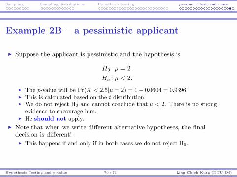
Example 2B – a pessimistic applicant
I Suppose the applicant is pessimistic and the hypothesis is
H0 : µ = 2
Ha : µ < 2.
I The p-value will be Pr(X < 2.5|µ = 2) = 1− 0.0604 = 0.9396.I This is calculated based on the t distribution.I We do not reject H0 and cannot conclude that µ < 2. There is no strong
evidence to encourage him.I He should not apply.
I Note that when we write different alternative hypotheses, the finaldecision is different!I This happens if and only if in both cases we do not reject H0.
Hypothesis Testing and p-value 70 / 71 Ling-Chieh Kung (NTU IM)

Sampling Sampling distributions Hypothesis testing p-value, t test, and more
Summary
I To test the population mean µ:
σ2 Sample sizePopulation distribution
Normal Nonnormal
Knownn ≥ 30 z zn < 30 z Nonparametric
Unknownn ≥ 30 t or z zn < 30 t Nonparametric
I More parameters that may be tested:I Population proportion (z test).I Population variance (χ2 test).I Difference of two population means (t test).I Ratio of two population variances (F test).
Hypothesis Testing and p-value 71 / 71 Ling-Chieh Kung (NTU IM)

Simple regression Multiple regression Indicators, interaction Endogeneity, residuals Logistic regression
Statistics and Data Analysis for Engineers
Part 3:Regression Analysis
Ling-Chieh Kung
Department of Information ManagementNational Taiwan University
September 4, 2016
Regression Analysis 1 / 83 Ling-Chieh Kung (NTU IM)

Simple regression Multiple regression Indicators, interaction Endogeneity, residuals Logistic regression
Correlation and prediction
I We often try to find correlation among variables.
I For example, prices and sizes of houses:
House 1 2 3 4 5 6
Size (m2) 75 59 85 65 72 46Price ($1000) 315 229 355 261 234 216
House 7 8 9 10 11 12
Size (m2) 107 91 75 65 88 59Price ($1000) 308 306 289 204 265 195
I We may calculate their correlation coefficient as r = 0.729.
I Now given a house whose size is 100 m2, may we predict its price?
Regression Analysis 2 / 83 Ling-Chieh Kung (NTU IM)

Simple regression Multiple regression Indicators, interaction Endogeneity, residuals Logistic regression
Correlation among more than two variables
I Sometimes we have more than two variables:
I For example, we may also know the number of bedrooms in each house:
House 1 2 3 4 5 6
Size (m2) 75 59 85 65 72 46Price ($1000) 315 229 355 261 234 216
Bedroom 1 1 2 2 2 1
House 7 8 9 10 11 12
Size (m2) 107 91 75 65 88 59Price ($1000) 308 306 289 204 265 195
Bedroom 3 3 2 1 3 1
I How to summarize the correlation among the three variables?
I How to predict house price based on size and number of bedrooms?
Regression Analysis 3 / 83 Ling-Chieh Kung (NTU IM)

Simple regression Multiple regression Indicators, interaction Endogeneity, residuals Logistic regression
Regression analysis
I Regression is a solution!
I As one of the most widely used tools in Statistics, it discovers:I Which variables affect a given variable.I How they affect the target.
I In general, we will predict/estimate one dependent variable by oneor multiple independent variables.I Independent variables: Potential factors that may affect the outcome.I Dependent variable: The outcome.I Independent variables are explanatory variables; the dependent variable
is the response variable.
I As another example, suppose we want to predict the number of arrivalconsumers for tomorrow:I Dependent variable: Number of arrival consumers.I Independent variables: Weather, holiday or not, promotion or not, etc.
Regression Analysis 4 / 83 Ling-Chieh Kung (NTU IM)
Simple regression Multiple regression Indicators, interaction Endogeneity, residuals Logistic regression
Types of regression analysis
I Based on the number of independent variables:I Simple regression: One independent variable.I Multiple regression: More than one independent variables.
I The dependent variable may be quantitative or qualitative.I In ordinary regression, the dependent variable is quantitative.I In logistic regression, the dependent variable is qualitative.
I There are other types of regression models.
Regression Analysis 5 / 83 Ling-Chieh Kung (NTU IM)

Simple regression Multiple regression Indicators, interaction Endogeneity, residuals Logistic regression
Road map
I Simple regression.
I Multiple regression.
I Indicator variables and interaction.
I Endogeneity and residual analysis.
I Logistic regression.
Regression Analysis 6 / 83 Ling-Chieh Kung (NTU IM)

Simple regression Multiple regression Indicators, interaction Endogeneity, residuals Logistic regression
Basic principleI Consider the price-size relationship again. In the sequel, let xi be the
size and yi be the price of house i, i = 1, ..., 12.
Size Price(in m2) (in $1000)
46 21659 22959 19565 26165 20472 23475 31575 28985 35588 26591 306107 308
I How to relate sizes and prices “in the best way?”
Regression Analysis 7 / 83 Ling-Chieh Kung (NTU IM)

Simple regression Multiple regression Indicators, interaction Endogeneity, residuals Logistic regression
Linear estimation
I If we believe that the relationship between the two variables is linear,we will assume that
yi = β0 + β1xi + εi.
I β0 is the intercept of the equation.I β1 is the slope of the equation.I εi is the random noise for estimating record i.
I Somehow there is such a formula, but we do not know β0 and β1.I β0 and β1 are the parameter of the population.I We want to use our sample data (e.g., the information of the twelve
houses) to estimate β0 and β1.I We want to form two statistics β0 and β1 as our estimates of β0 and β1.
Regression Analysis 8 / 83 Ling-Chieh Kung (NTU IM)

Simple regression Multiple regression Indicators, interaction Endogeneity, residuals Logistic regression
Linear estimationI Given the values of β0 and β1, we will use yi = β0 + β1xi as our
estimate of yi.
I Then we haveyi = β0 + β1xi + εi,
where εi is now interpreted as the estimation error.I Let yi = β0 + β1xi be our estimate of yi. We hope εi = yi− yi to be small.
I For all data points, let’s minimize the sum of squared errors (SSE):
n∑i=1
ε2i = (yi − yi)2 =
n∑i=1
[(yi − (β0 + β1xi)
]2.
I The solution of
minβ0,β1
n∑i=1
[(yi − (β0 + β1xi)
]2is our least square approximation (estimation) of the given data.
Regression Analysis 9 / 83 Ling-Chieh Kung (NTU IM)

Simple regression Multiple regression Indicators, interaction Endogeneity, residuals Logistic regression
Least square approximation
I The least square approximation problem
minβ0,β1
n∑i=1
[(yi − (β0 + β1xi)
]2has a closed-form formula for the best (β0, β1):
β1 =
∑ni=1(xi − x)(yi − y)∑n
i=1(xi − x)2and β0 = y − β1x.
I For our house example, we will get (β0, β1) = (102.717, 2.192).I Its SSE is 13118.63.I We will never know the true values of β0 and β1. However, according to
our sample data, the best (least square) estimate is (102.717, 2.192).I We tend to believe that β0 = 102.717 and β1 = 2.192.
Regression Analysis 10 / 83 Ling-Chieh Kung (NTU IM)

Simple regression Multiple regression Indicators, interaction Endogeneity, residuals Logistic regression
Interpretations
I Our regression model is
y = 102.717 + 2.192x.
I Interpretation: When the housesize increases by 1 m2, the price isexpected to increase by $2, 192.
I (Bad) interpretation: For a housewhose size is 0 m2, the price isexpected to be $102,717.
Regression Analysis 11 / 83 Ling-Chieh Kung (NTU IM)

Simple regression Multiple regression Indicators, interaction Endogeneity, residuals Logistic regression
Linear multiple regression
I In most cases, more than one independent variable may be used toexplain the outcome of the dependent variable.
I For example, consider the number of bedrooms.
I We may take both variables asindependent variables to do linearmultiple regression:
yi = β0 + β1x1,i + β2x2,i + εi.
I yi is the house price (in $1000).I x1,i is the house size (in m2).I x2,i is the number of bedrooms.I εi is the random noise.
I Our (least square) estimate is
(β0, β1, β2) = (82.737, 2.854,−15.789).
Price SizeBedroom
(in $1000) (in m2)
315 75 1229 59 1355 85 2261 65 2234 72 2216 46 1308 107 3306 91 3289 75 2204 65 1265 88 3195 59 1
Regression Analysis 12 / 83 Ling-Chieh Kung (NTU IM)

Simple regression Multiple regression Indicators, interaction Endogeneity, residuals Logistic regression
InterpretationsI Our regression model is
y = 82.737 + 2.854x1 − 15.789x2.
I When the house size increases by 1 m2 (and all other independentvariables are fixed), we expect the price to increase by $2, 854.
I When there is one more bedroom (and all other independent variablesare fixed), we expect the price to decrease by $15, 789.
I One must interpret the results and determine whether the result ismeaningful by herself/himself.I The number of bedrooms may not be a good indicator of house price.I At least not in a linear way.
I We need more than finding coefficients:I We need to judge the overall quality of a given regression model.I We may want to compare multiple regression models.I We must test the significance of regression coefficients.
Regression Analysis 13 / 83 Ling-Chieh Kung (NTU IM)

Simple regression Multiple regression Indicators, interaction Endogeneity, residuals Logistic regression
Model validation: How good is a model?I How to measure the quality of a model?I For the model y = 102.717 + 2.192x, how good is it?I In general, for a given regression model y = β0 + β1x1 + · · · βkxk, how
may we evaluate its overall quality?I The sum of squared total errors (SST), SST =
∑ni=1(yi − y)2, is
for the worst model.I With our regression model, the sum of squared errors (SSE) is
SSE =
n∑i=1
(yi − yi)2 =
n∑i=1
[(yi − (β0 + β1xi)
]2.
I The proportion of total variability that is explained by the regressionmodel is
0 ≤ R2 = 1− SSE
SST≤ 1.
The larger R2, the better the regression model.
Regression Analysis 14 / 83 Ling-Chieh Kung (NTU IM)

Simple regression Multiple regression Indicators, interaction Endogeneity, residuals Logistic regression
Obtaining R2
I Whenever we find the estimated coefficients, we have R2.
I Statistical software includes R2 in the regression report.
I For the regression model y = 102.717 + 2.192x, we have R2 = 0.5315:I Around 53% of a house price is determined by its house size.
I If (and only if) there is only one independent variable, then R2 = r2,where r is the correlation coefficient between the dependent andindependent variables.I −1 ≤ r ≤ 1.I 0 ≤ r2 = R2 ≤ 1.
Regression Analysis 15 / 83 Ling-Chieh Kung (NTU IM)

Simple regression Multiple regression Indicators, interaction Endogeneity, residuals Logistic regression
Comparing regression models
I Now we have a way to compare regression models.
I For our example:
Size only Bedroom only Size and bedroom
R2 0.5315 0.29 0.5513
I Using prices only is better than using numbers of bedrooms only.I Is using prices and bedrooms better?
I In general, adding more variables always increases R2!I In the worst case, we may set the corresponding coefficients to 0.I Some variables may actually be meaningless.
I To perform a “fair” comparison and identify those meaningful factors,we need to adjust R2 based on the number of independent variables.
Regression Analysis 16 / 83 Ling-Chieh Kung (NTU IM)

Simple regression Multiple regression Indicators, interaction Endogeneity, residuals Logistic regression
Adjusted R2
I The standard way to adjust R2 to adjusted R2 is
R2adj = 1−
(n− 1
n− k − 1
)(1−R2).
I n is the sample size and k is the number of independent variables used.
I For our example:
Size only Bedroom only Size and bedroom
R2 0.5315 0.290 0.5513R2
adj 0.4846 0.219 0.4516
I Actually using sizes only results in the best model!
Regression Analysis 17 / 83 Ling-Chieh Kung (NTU IM)
Simple regression Multiple regression Indicators, interaction Endogeneity, residuals Logistic regression
Testing coefficient significance
I Another important task for validating a regression model is to test thesignificance of each coefficient.
I Recall our model with two independent variables
y = 82.737 + 2.854x1 − 15.789x2.
I Note that 2.854 and −15.789 are solely calculated based on the sample.We never know whether β1 and β2 are really these two values!
I In fact, we cannot even be sure that β1 and β2 are not 0. We need totest them:
H0 : βi = 0
Ha : βi 6= 0.
I We look for a strong enough evidence showing that βi 6= 0.
Regression Analysis 18 / 83 Ling-Chieh Kung (NTU IM)

Simple regression Multiple regression Indicators, interaction Endogeneity, residuals Logistic regression
Testing coefficient significance
I The testing results are provided in regression reports.
I Statistical software (e.g., R) tells us:
Coefficients Standard Error t Stat p-value
Intercept 82.737 59.873 1.382 0.200Size 2.854 1.247 2.289 0.048 **Bedroom −15.789 25.056 −0.630 0.544
I As we have no idea about population variance, we apply the t test.I “Coefficients” records sample means x; “Standard Error” records S√
n; “t
Stat” records T = x−0S/√n
.I “p-value” are the tail probabilities of T multiplied by 2 (done by most
software). Simply compare them with α!
I Recall the assumption that εi is normal!
Regression Analysis 19 / 83 Ling-Chieh Kung (NTU IM)

Simple regression Multiple regression Indicators, interaction Endogeneity, residuals Logistic regression
Testing coefficient significance
I Statistical software tells us:
Coefficients Standard Error t Stat p-value
Intercept 82.737 59.873 1.382 0.200Size 2.854 1.247 2.289 0.048 **Bedroom −15.789 25.056 −0.630 0.544
I At a 95% confidence level, we believe that β1 6= 0. House size really hassome impact on house price.
I At a 95% confidence level, we have no evidence for β2 6= 0. We cannotconclude that the number of bedrooms has an impact on house price.
I If we use only size as an independent variable, its p-value will be0.00714. We will be quite confident that it has an impact.
Regression Analysis 20 / 83 Ling-Chieh Kung (NTU IM)
Simple regression Multiple regression Indicators, interaction Endogeneity, residuals Logistic regression
Road map
I Simple regression.
I Multiple regression.
I Indicator variables and interaction.
I Endogeneity and residual analysis.
I Logistic regression.
Regression Analysis 21 / 83 Ling-Chieh Kung (NTU IM)

Simple regression Multiple regression Indicators, interaction Endogeneity, residuals Logistic regression
House age
I The age of a house may also affect its price.
Price SizeBedroom
Age(in $1000) (in m2) (in years)
315 75 1 16229 59 1 20355 85 2 16261 65 2 15234 72 2 21216 46 1 16308 107 3 15306 91 3 15289 75 2 14204 65 1 21265 88 3 15195 59 1 26
I Let’s add age as an independent variable in explaining house prices.I Because the number of bedroom seems to be unhelpful, let’s ignore it.
Regression Analysis 22 / 83 Ling-Chieh Kung (NTU IM)
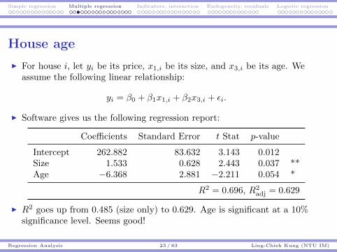
Simple regression Multiple regression Indicators, interaction Endogeneity, residuals Logistic regression
House age
I For house i, let yi be its price, x1,i be its size, and x3,i be its age. Weassume the following linear relationship:
yi = β0 + β1x1,i + β2x3,i + εi.
I Software gives us the following regression report:
Coefficients Standard Error t Stat p-value
Intercept 262.882 83.632 3.143 0.012Size 1.533 0.628 2.443 0.037 **Age −6.368 2.881 −2.211 0.054 *
R2 = 0.696, R2adj = 0.629
I R2 goes up from 0.485 (size only) to 0.629. Age is significant at a 10%significance level. Seems good!
Regression Analysis 23 / 83 Ling-Chieh Kung (NTU IM)

Simple regression Multiple regression Indicators, interaction Endogeneity, residuals Logistic regression
“Nonlinear” relationship
I May we do better?
I By looking at the age-price scatter plot(and our intuition), maybe the impact ofage on price is “nonlinear”:I A new house’s value depreciates fast.I The value depreciates slowly when the
house is old.I At least this is true for a car.
I It is worthwhile to try a capture thisnonlinear relationship.
I For example, we may try to replace houseage by its reciprocal:
yi = β0 + β1x1,i + β2
(1
x3,i
)+ εi.
Regression Analysis 24 / 83 Ling-Chieh Kung (NTU IM)
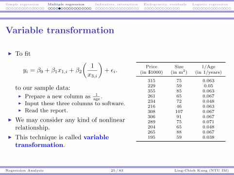
Simple regression Multiple regression Indicators, interaction Endogeneity, residuals Logistic regression
Variable transformation
I To fit
yi = β0 + β1x1,i + β2
(1
x3,i
)+ εi.
to our sample data:I Prepare a new column as 1
age.
I Input these three columns to software.I Read the report.
I We may consider any kind of nonlinearrelationship.
I This technique is called variabletransformation.
Price Size 1/Age(in $1000) (in m2) (in 1/years)
315 75 0.063229 59 0.05355 85 0.063261 65 0.067234 72 0.048216 46 0.063308 107 0.067306 91 0.067289 75 0.071204 65 0.048265 88 0.067195 59 0.038
Regression Analysis 25 / 83 Ling-Chieh Kung (NTU IM)
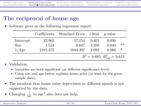
Simple regression Multiple regression Indicators, interaction Endogeneity, residuals Logistic regression
The reciprocal of house ageI Software gives us the following regression report:
Coefficients Standard Error t Stat p-value
Intercept 22.905 57.154 0.401 0.698Size 1.524 0.647 2.356 0.043 **1/Age 2185.575 1044.497 2.092 0.066 *
R2 = 0.685, R2adj = 0.615
I Validation:I Variables are both significant (at different significance level).I Using size and age better explains house price (at least for the given
sample data).
I The intuition that house value depreciates at different speeds is notsupported by the data.
I Changing 1age to age2 also does not help.
Regression Analysis 26 / 83 Ling-Chieh Kung (NTU IM)

Simple regression Multiple regression Indicators, interaction Endogeneity, residuals Logistic regression
Typical ways of variable transformation
Regression Analysis 27 / 83 Ling-Chieh Kung (NTU IM)
Simple regression Multiple regression Indicators, interaction Endogeneity, residuals Logistic regression
Variable selection and model building
I In general, we may have a lot of candidate independent variables.I Size, number of bedrooms, age, distance to a park, distance to a hospital,
safety in the neighborhood, etc.I If we consider only linear relationships, for p candidate independent
variables, we have 2p − 1 combinations.I For each variable, we have many ways to transform it.I In the next lecture, we will introduce the way of modeling interaction
among independent variables.
I How to find the “best” regression model (if there is one)?
Regression Analysis 28 / 83 Ling-Chieh Kung (NTU IM)

Simple regression Multiple regression Indicators, interaction Endogeneity, residuals Logistic regression
Variable selection and model buildingI There is no “best” model; there are “good” models.I Some general suggestions:
I Take each independent variable one at a time and observe therelationship between it and the dependent variable. A scatter plothelps. Use this to consider variable transformation.
I For each pair of independent variables, check their relationship. If twoare highly correlated, quite likely one is not needed.
I Once a model is built, check the p-values. You may want to removeinsignificant variables (but removing a variable may change thesignificance of other variables).
I Go back and forth to try various combinations. Stop when a goodenough one (with high R2 and R2
adj and small p-values) is found.I Software can somewhat automate the process, but its power is limited
(e.g., it cannot decide transformation).I We may need to find new independent variables.
I Intuitions and experiences may help (or hurt).
Regression Analysis 29 / 83 Ling-Chieh Kung (NTU IM)
Simple regression Multiple regression Indicators, interaction Endogeneity, residuals Logistic regression
Summary
I With a regression model, we try to identify how independent variablesaffect the dependent variable.I For a regression model, we adopt the least square criterion for estimating
the coefficients.
I Model validation:I The overall quality of a regression model is decided by its R2 and R2
adj.I We may test the significance of independent variables by their p-values.
I Modeling building:I Variable transformation.I Variable selection.
Regression Analysis 30 / 83 Ling-Chieh Kung (NTU IM)

Simple regression Multiple regression Indicators, interaction Endogeneity, residuals Logistic regression
Case study: ticket selling
I A theater made hundreds of stage performances in the past six years.
I The owner hopes that statistics and data analysis may help herimprove the ticket sales.
I Key questions: What makes a show popular?I Popularity is defined as the numbers of tickets sold.I Potential factors: year, month, day, time, location, actors/actresses,
drama type, ticket prices, etc.
I 100 performances are randomly drawn from the whole pool.I All were made during weekends.I Tickets were all publicly sold.I Tickets for all performances were sold through the same channels.I For each performance, the ticket price(s) remained the same.
I As a group of consultants, how may we help the theater?
Regression Analysis 31 / 83 Ling-Chieh Kung (NTU IM)

Simple regression Multiple regression Indicators, interaction Endogeneity, residuals Logistic regression
Variables
I Six variables are obtained:
Variable Meaning
Year The year in which the performance was madeTime Morning, afternoon, or evening
Capacity The number of seats in the theater hallAvgPrice The average of all pricesSalesQty The number of tickets sold
SalesDuration Performance day − Announcement day
I Labeling and scaling:I Years are labeled as 1, 2, ..., and 6 (6 means the last year).I Capacities and sales quantities have been scaled in the same proportion.
Regression Analysis 32 / 83 Ling-Chieh Kung (NTU IM)

Simple regression Multiple regression Indicators, interaction Endogeneity, residuals Logistic regression
Data (incomplete)
Yr. Tm. Cap. A.P. Qty S.D. Yr. Tm. Cap. A.P. Qty S.D.
5 A 230 400 218 50 2 M 190 575 190 2895 A 150 500 119 46 6 A 130 500 108 895 A 230 400 160 126 4 E 200 775 169 1005 A 200 775 200 324 4 E 200 775 135 2596 E 190 1175 178 115 5 A 310 650 251 3466 A 190 1175 183 109 2 A 250 550 250 1455 E 190 775 161 58 1 A 190 675 183 2543 A 200 675 200 112 6 A 200 1175 146 1105 E 200 775 158 323 1 M 200 575 140 941 M 200 575 128 360 4 A 200 775 195 255
Regression Analysis 33 / 83 Ling-Chieh Kung (NTU IM)
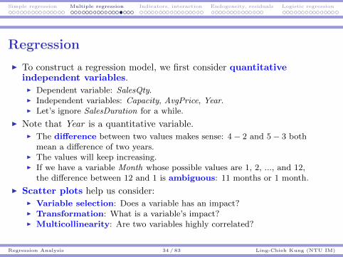
Simple regression Multiple regression Indicators, interaction Endogeneity, residuals Logistic regression
Regression
I To construct a regression model, we first consider quantitativeindependent variables.I Dependent variable: SalesQty.I Independent variables: Capacity, AvgPrice, Year.I Let’s ignore SalesDuration for a while.
I Note that Year is a quantitative variable.I The difference between two values makes sense: 4− 2 and 5− 3 both
mean a difference of two years.I The values will keep increasing.I If we have a variable Month whose possible values are 1, 2, ..., and 12,
the difference between 12 and 1 is ambiguous: 11 months or 1 month.
I Scatter plots help us consider:I Variable selection: Does a variable has an impact?I Transformation: What is a variable’s impact?I Multicollinearity: Are two variables highly correlated?
Regression Analysis 34 / 83 Ling-Chieh Kung (NTU IM)

Simple regression Multiple regression Indicators, interaction Endogeneity, residuals Logistic regression
Regression Analysis 35 / 83 Ling-Chieh Kung (NTU IM)

Simple regression Multiple regression Indicators, interaction Endogeneity, residuals Logistic regression
Regression
I It seems that Capacity, AvgSales, and Year are all worth a try.
I Let’s put them into a regression model.
I If we do this one by one:I SalesQty = 20.79 + 0.72Capacity: R2 = 0.538, p-value ≈ 0.I SalesQty = 174.9 + 0.0028AvgPrice: R2 = 0.0002, p-value = 0.885.I SalesQty = 203.6− 6.77Y ear: R2 = 0.063, p-value = 0.0115.
I If we include them together:I The regression model is
SalesQty = 24.742 + 0.702Capacity + 0.027AvgPrice− 4.696Y ear.
I R2 = 0.57, R2adj = 0.556; p-values are 0, 0.056, and 0.019, respectively.
I Do not try independent variables separately; try them together.
Regression Analysis 36 / 83 Ling-Chieh Kung (NTU IM)
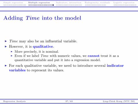
Simple regression Multiple regression Indicators, interaction Endogeneity, residuals Logistic regression
Adding Time into the model
I Time may also be an influential variable.
I However, it is qualitative.I More precisely, it is nominal.I Even if we label Time with numeric values, we cannot treat it as a
quantitative variable and put it into a regression model.
I For each qualitative variable, we need to introduce several indicatorvariables to represent its values.
Regression Analysis 37 / 83 Ling-Chieh Kung (NTU IM)

Simple regression Multiple regression Indicators, interaction Endogeneity, residuals Logistic regression
Road map
I Simple regression.
I Multiple regression.
I Indicator variables and interaction.
I Endogeneity and residual analysis.
I Logistic regression.
Regression Analysis 38 / 83 Ling-Chieh Kung (NTU IM)
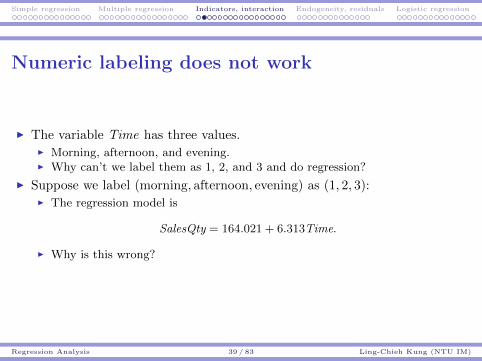
Simple regression Multiple regression Indicators, interaction Endogeneity, residuals Logistic regression
Numeric labeling does not work
I The variable Time has three values.I Morning, afternoon, and evening.I Why can’t we label them as 1, 2, and 3 and do regression?
I Suppose we label (morning, afternoon, evening) as (1, 2, 3):I The regression model is
SalesQty = 164.021 + 6.313Time.
I Why is this wrong?
Regression Analysis 39 / 83 Ling-Chieh Kung (NTU IM)

Simple regression Multiple regression Indicators, interaction Endogeneity, residuals Logistic regression
Numeric labeling does not work
I Different labeling gives different regression results.
I We may also label (morning, afternoon, evening) as (1, 2, 10) or (3, 1, 2):
SalesQty =
164.021 + 6.313Time
p-value = 0.294
SalesQty =
177.224− 0.075Time
p-value = 0.95
SalesQty =
205.725− 15.091Time
p-value = 0.0084
Regression Analysis 40 / 83 Ling-Chieh Kung (NTU IM)
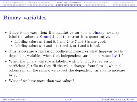
Simple regression Multiple regression Indicators, interaction Endogeneity, residuals Logistic regression
Binary variables
I There is one exception: If a qualitative variable is binary, we maylabel the values as 0 and 1 and then treat it as quantitative.I Labeling values as 1 and 0, 1 and 2, or 7 and 8 is also good.I Labeling values as 1 and −1, 1 and 5, or 4 and 8 is bad.
I This is because a regression coefficient measures what happens to thedependent variable “when that independent variable increases by 1.”
I When the binary variable is labeled with 0 and 1, its regressioncoefficient βi tells us that “if the value changes from 0 to 1 (while allothers remain the same), we expect the dependent variable to increase
by βi.”
I What if we have more than two values?
Regression Analysis 41 / 83 Ling-Chieh Kung (NTU IM)

Simple regression Multiple regression Indicators, interaction Endogeneity, residuals Logistic regression
Indicator variables
I Consider a variable x with three values A, B, and C.
I We first choose a reference level, say, A.
I We then manually create two indicator variables xB and xC :
xB =
{1 if x = B
0 otherwiseand xC =
{1 if x = C
0 otherwise
In other words, we have a mapping:
x xB xC
A 0 0B 1 0C 0 1
Regression Analysis 42 / 83 Ling-Chieh Kung (NTU IM)
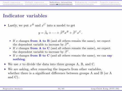
Simple regression Multiple regression Indicators, interaction Endogeneity, residuals Logistic regression
Indicator variables
I Lastly, we put xB and xC into a model to get
y = β0 + · · ·+ βBxB + βCxC .
I If x changes from A to B (and all others remain the same), we expectthe dependent variable to increase by βB .
I If x changes from A to C (and all others remain the same), we expectthe dependent variable to increase by βC .
I If x changes from B to C (and all others remain the same), we can saynothing.
I We use x to divide the data into three groups A, B, and C.
I We are asking, after removing the impacts from other variables,whether there is a significant difference between groups A and B (or Aand C).
Regression Analysis 43 / 83 Ling-Chieh Kung (NTU IM)
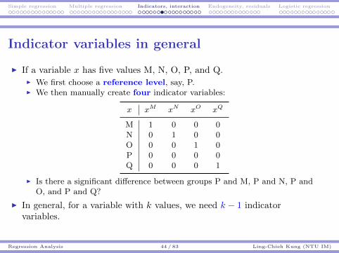
Simple regression Multiple regression Indicators, interaction Endogeneity, residuals Logistic regression
Indicator variables in general
I If a variable x has five values M, N, O, P, and Q.I We first choose a reference level, say, P.I We then manually create four indicator variables:
x xM xN xO xQ
M 1 0 0 0N 0 1 0 0O 0 0 1 0P 0 0 0 0Q 0 0 0 1
I Is there a significant difference between groups P and M, P and N, P andO, and P and Q?
I In general, for a variable with k values, we need k − 1 indicatorvariables.
Regression Analysis 44 / 83 Ling-Chieh Kung (NTU IM)
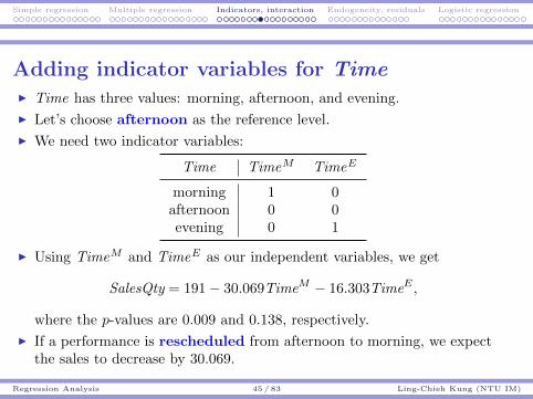
Simple regression Multiple regression Indicators, interaction Endogeneity, residuals Logistic regression
Adding indicator variables for TimeI Time has three values: morning, afternoon, and evening.
I Let’s choose afternoon as the reference level.
I We need two indicator variables:
Time TimeM TimeE
morning 1 0afternoon 0 0evening 0 1
I Using TimeM and TimeE as our independent variables, we get
SalesQty = 191− 30.069TimeM − 16.303TimeE ,
where the p-values are 0.009 and 0.138, respectively.
I If a performance is rescheduled from afternoon to morning, we expectthe sales to decrease by 30.069.
Regression Analysis 45 / 83 Ling-Chieh Kung (NTU IM)

Simple regression Multiple regression Indicators, interaction Endogeneity, residuals Logistic regression
Adding indicator variables for Time
I Let’s include Capacity, AvgPrice, Year, TimeM , and TimeE :
SalesQty = 0.696Capacity + 0.027AvgPrice− 5.282Year
− 14.387TimeM − 21.328TimeE .
Coefficients Standard Error t Stat p-value
Intercept 39.280 19.724 1.992 0.049 **Capacity 0.696 0.069 10.263 0.000 ***AvgPrice 0.027 0.013 2.033 0.045 **Year −5.282 1.931 −2.735 0.007 ***TimeM −14.387 7.784 −1.848 0.068 *TimeE −21.328 7.227 −2.951 0.004 ***
R2 = 0.608, R2adj = 0.587
Regression Analysis 46 / 83 Ling-Chieh Kung (NTU IM)
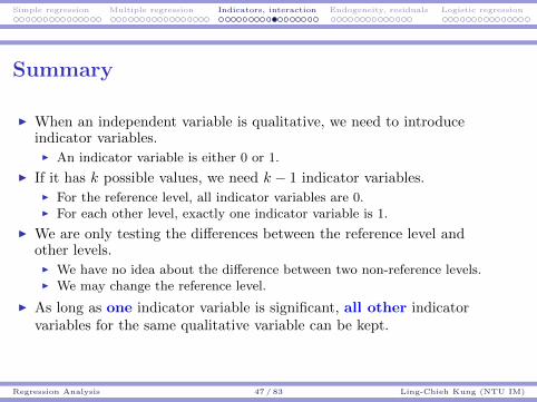
Simple regression Multiple regression Indicators, interaction Endogeneity, residuals Logistic regression
Summary
I When an independent variable is qualitative, we need to introduceindicator variables.I An indicator variable is either 0 or 1.
I If it has k possible values, we need k − 1 indicator variables.I For the reference level, all indicator variables are 0.I For each other level, exactly one indicator variable is 1.
I We are only testing the differences between the reference level andother levels.I We have no idea about the difference between two non-reference levels.I We may change the reference level.
I As long as one indicator variable is significant, all other indicatorvariables for the same qualitative variable can be kept.
Regression Analysis 47 / 83 Ling-Chieh Kung (NTU IM)
Simple regression Multiple regression Indicators, interaction Endogeneity, residuals Logistic regression
Interaction among variables
I In a regression model
y = β0 + β1x1 + β2x2 + · · ·βpxp,
βi measures how xi affects y.
I Sometimes the impact of xi on y depends on the value of anothervariable xj .
I Consider house prices, sizes, and numbers of bedrooms.I When a house is big, more numbers of bedrooms may be good.I When a house is small, more numbers of bedrooms may be bad.
I Consider the demand of a product.I Demand is sensitive to price: When price goes up, demand goes down.I The sensitivity may be different between men and women.
I In this case, we say there is an interaction between xi and xj .
Regression Analysis 48 / 83 Ling-Chieh Kung (NTU IM)

Simple regression Multiple regression Indicators, interaction Endogeneity, residuals Logistic regression
Modeling interaction
I To model the interaction between xi and xj , one possibility is to createa new variable xixj , which is the product of the two original variables.
I In a regression model
y = β0 + β1x1 + β2x2 + β1,2x1x2 · · · ,
β1,2 measures the interaction between x1 and x2.I The impact of x1 on y is β1 + β1,2x2.I The impact of x2 on y is β2 + β1,2x1.
I A quadratic term x2i in a regression model
y = β0 + β1x1 + β′1x21 + · · · ,
is a special case: The impact of x1 on y is depends on the value of x1.
Regression Analysis 49 / 83 Ling-Chieh Kung (NTU IM)

Simple regression Multiple regression Indicators, interaction Endogeneity, residuals Logistic regression
Interaction between Time and AvgPrice
I Do Time and AvgPrice affect each other’s impact?
I Let’s add TimeM ×AvgPrice and TimeE ×AvgPrice into our model:
Coefficients Std. Error t Stat p-value
Intercept 55.876 22.652 2.467 0.015 **Capacity 0.676 0.068 9.950 0.000 ***Year −6.192 1.966 −3.149 0.002 ***TimeM −55.205 23.829 −2.317 0.023 **TimeE −19.105 21.81 −0.876 0.383AvgPrice 0.015 0.019 0.836 0.405TimeM ×AvgPrice 0.054 0.030 1.792 0.076 *TimeE ×AvgPrice −0.004 0.030 −0.136 0.892
R2 = 0.624, R2adj = 0.595
I If we want to keep TimeE ×AvgPrice, we must also keepTimeM ×AvgPrice, AvgPrice, TimeM , and TimeE in our model.
Regression Analysis 50 / 83 Ling-Chieh Kung (NTU IM)
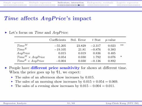
Simple regression Multiple regression Indicators, interaction Endogeneity, residuals Logistic regression
Time affects AvgPrice’s impact
I Let’s focus on Time and AvgPrice:
Coefficients Std. Error t Stat p-value
TimeM −55.205 23.829 −2.317 0.023 **TimeE −19.105 21.81 −0.876 0.383AvgPrice 0.015 0.019 0.836 0.405TimeM ×AvgPrice 0.054 0.030 1.792 0.076 *TimeE ×AvgPrice −0.004 0.030 −0.136 0.892
I People have different price sensitivity for shows at different time.When the price goes up by $1, we expect:I The sales of an afternoon show increases by 0.015.I The sales of an morning show increases by 0.015 + 0.054 = 0.069.I The sales of a evening show increases by 0.015− 0.004 = 0.011.
Regression Analysis 51 / 83 Ling-Chieh Kung (NTU IM)
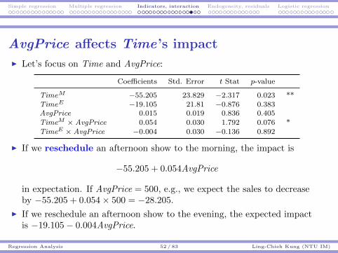
Simple regression Multiple regression Indicators, interaction Endogeneity, residuals Logistic regression
AvgPrice affects Time’s impact
I Let’s focus on Time and AvgPrice:
Coefficients Std. Error t Stat p-value
TimeM −55.205 23.829 −2.317 0.023 **TimeE −19.105 21.81 −0.876 0.383AvgPrice 0.015 0.019 0.836 0.405TimeM ×AvgPrice 0.054 0.030 1.792 0.076 *TimeE ×AvgPrice −0.004 0.030 −0.136 0.892
I If we reschedule an afternoon show to the morning, the impact is
−55.205 + 0.054AvgPrice
in expectation. If AvgPrice = 500, e.g., we expect the sales to decreaseby −55.205 + 0.054× 500 = −28.205.
I If we reschedule an afternoon show to the evening, the expected impactis −19.105− 0.004AvgPrice.
Regression Analysis 52 / 83 Ling-Chieh Kung (NTU IM)

Simple regression Multiple regression Indicators, interaction Endogeneity, residuals Logistic regression
Interaction between Time affects YearI Do Time and Year affect each other’s impact?
Coefficients Std. Error t Stat p-value
(Intercept) 39.597 22.31 1.775 0.079 *Capacity 0.693 0.068 10.267 0.000 ***AvgPrice 0.024 0.013 1.799 0.075 *TimeE −2.696 18.562 −0.145 0.885TimeM −25.114 18.303 −1.372 0.173Year −4.703 2.944 −1.597 0.114TimeE ×Year −4.841 4.302 −1.125 0.263TimeM ×Year 2.898 4.166 0.695 0.489
R2 = 0.620, R2adj = 0.591
I All the five variables related to Time and Year are insignificant.I People’s preference over the show time do not change from year to year.I The trend from year to year is the same for different show times.
I Though all the five variables are insignificant, we typically first try toremove only the interaction terms.
Regression Analysis 53 / 83 Ling-Chieh Kung (NTU IM)

Simple regression Multiple regression Indicators, interaction Endogeneity, residuals Logistic regression
Summary
I Two variables’ interaction may be modeled with a product term.I If its coefficient is significantly nonzero, one variable’s impact depends on
the other’s value.
I Three rules for keeping variables:I Quadratic transformation: If we want to keep x2, we must also keep x.I Indicator variable: If we want to keep xk
′, where xk
′is the indicator
variable for represent x = k′, we must also keep xk for all k 6= k′.I Interaction: If we want to keep xixj , we must also keep xi and xj .
I Therefore:I If we want to have xix
k′j , where xk
′j is the indicator variable for represent
xj = k′, we must also keep xkj for all k 6= k′.
I It is possible to add xixjxk into a regression model.
Regression Analysis 54 / 83 Ling-Chieh Kung (NTU IM)

Simple regression Multiple regression Indicators, interaction Endogeneity, residuals Logistic regression
Road map
I Simple regression.
I Multiple regression.
I Indicator variables and interaction.
I Endogeneity and residual analysis.
I Logistic regression.
Regression Analysis 55 / 83 Ling-Chieh Kung (NTU IM)
Simple regression Multiple regression Indicators, interaction Endogeneity, residuals Logistic regression
SalesDuration
I Consider the variable SalesDuration.I The difference between the announce day and performance day.I The number of days that the tickets for a show are publicly sold.I The longer sales duration, the more sales?
I We probably want to add SalesDuration into our regression model.
I This is problematic in this case:I Typically the theater determines its schedule for the next year at the end
of each year.I Most performances are scheduled.I Ticket selling starts a few months before a series of shows are performed.I However, if a series turns out to be popular, the theater may decide to
add more shows into this series.I These additional shows have much shorter SalesDuration and typically
have high SalesQty.
I In short, SalesQty affects SalesDuration.
Regression Analysis 56 / 83 Ling-Chieh Kung (NTU IM)
Simple regression Multiple regression Indicators, interaction Endogeneity, residuals Logistic regression
Endogeneity
I If in a regression model an independent variable is affected by thedependent variable, we say the model has the endogeneity problem.I If we add SalesDuration into our model, we creates endogeneity.I Year, Time, Capacity, and AvgPrice do not have the endogeneity
problem.I If any of them may be modified when the theater sees a good (or bad)
sales, endogeneity emerges.
I Endogeneity results in a biased prediction.
I In our ticket selling example, if we add SalesDuration into our model,we may intentionally announce shows later!
Regression Analysis 57 / 83 Ling-Chieh Kung (NTU IM)

Simple regression Multiple regression Indicators, interaction Endogeneity, residuals Logistic regression
Example: promotional phone calls
I A bank lets its workers call people to invite them to deposit money.
I Many factors may affect the outcome (success or not):1
I The callee’ gender, age, occupation, education level, etc.I The caller’s gender, age, experience, etc.I The calling day, calling time, weather at the call, etc.
I All these information from past calls are recorded.
I The length of each call is also recorded.I It is found to be highly correlated with success/failure.I However, it cannot be used as an independent variable.I Because it is affected by the outcome: Once one agrees to deposit
money, the call gets longer to talk about more details.
I In this example, if we add call duration into our model, we may askour workers to speak as slowly as possible.
1A regression model that incorporates a qualitative dependent variable will beintroduced in later lectures.
Regression Analysis 58 / 83 Ling-Chieh Kung (NTU IM)
Simple regression Multiple regression Indicators, interaction Endogeneity, residuals Logistic regression
Avoiding endogeneity
I To avoid endogeneity:I Remove the independent variable is endogenous.I Remove those records in which an independent variable is affected by
the dependent one.
I In the ticket selling example:I We may remove SalesDuration.I We may remove those additional shows.
I In the promotional call example:I We may remove the variable of call duration.
Regression Analysis 59 / 83 Ling-Chieh Kung (NTU IM)

Simple regression Multiple regression Indicators, interaction Endogeneity, residuals Logistic regression
Introduction
I When doing regression:I We try to discover the hidden relationship among variables.I We assume a specific model
y = β0 + β1x1 + · · ·+ ε
and then fit our sample data to the model.I We validate our model based on the degree of fitness (R2 and R2
adj)and significance of variables (p-values).
I If our model is good, the random error ε should be really “random.”I There should be no systematic pattern for ε.
I We need residual analysis.
Regression Analysis 60 / 83 Ling-Chieh Kung (NTU IM)

Simple regression Multiple regression Indicators, interaction Endogeneity, residuals Logistic regression
Residuals
I Consider a pair of variables x and y.
I We may assume a linear relationship
y = β0 + β1x+ ε
for some unknown parameters β0 and β1. ε is the random error.
I Four assumptions on the random error:I Zero mean: The expected value of ε is zero for any value of x.I Constant variance: The variance of ε is the same for any value of x.I Independence: ε for different values of x should be independent.I Normality: ε is normal for any value of x.
I Once we obtain a regression model, we need to test these assumptions.I To predict: We need the first three.I To explain: We need all the four.
Regression Analysis 61 / 83 Ling-Chieh Kung (NTU IM)

Simple regression Multiple regression Indicators, interaction Endogeneity, residuals Logistic regression
Testing the four assumptions
I Consider a sample data set {(xi, yi)}i=1,...,n.
I Linear regression helps us find β0 and β1 based on the sample data andobtain the regression formula
yi = β0 + β1xi + εi,
in which the error term εi is called the residual between our estimateyi = β0 + β1xi and the real value yi.
I By conducting a residual analysis, we check these εis to see if wehave the desired properties.
I While there are rigorous statistical tests, we will only introduce somegraphical approaches.
Regression Analysis 62 / 83 Ling-Chieh Kung (NTU IM)
Simple regression Multiple regression Indicators, interaction Endogeneity, residuals Logistic regression
The residual plot and histogram
I We may plot the residuals εis along with xis to form a residual plot.I This tests zero mean, constant variance, and independence.I There should be no systematic pattern.
I We may construct a histogram of residuals.I This tests normality.I The histogram should be symmetric and bell-shaped.
I In general:I A “good” plot does not guarantee a good model.I A “bad” plot strongly suggests that the model is bad!
Regression Analysis 63 / 83 Ling-Chieh Kung (NTU IM)
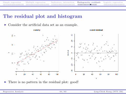
Simple regression Multiple regression Indicators, interaction Endogeneity, residuals Logistic regression
The residual plot and histogram
I Consider the artificial data set as an example.
I There is no pattern in the residual plot: good!
Regression Analysis 64 / 83 Ling-Chieh Kung (NTU IM)

Simple regression Multiple regression Indicators, interaction Endogeneity, residuals Logistic regression
The residual plot and histogram
I Consider the artificial data set as an example.
I The histogram is symmetric and bell-shaped: good!
Regression Analysis 65 / 83 Ling-Chieh Kung (NTU IM)

Simple regression Multiple regression Indicators, interaction Endogeneity, residuals Logistic regression
Residual plots that pass and fail the tests
Regression Analysis 66 / 83 Ling-Chieh Kung (NTU IM)

Simple regression Multiple regression Indicators, interaction Endogeneity, residuals Logistic regression
Histograms that pass and fail the tests
Regression Analysis 67 / 83 Ling-Chieh Kung (NTU IM)

Simple regression Multiple regression Indicators, interaction Endogeneity, residuals Logistic regression
Residual analysis for multiple regression
I Suppose that we construct a multiple regression model
yi = β0 + β1xi + · · ·+ βpxp + εi.
I We still use residual plots and a histogram to test the assumptions.
I Multiple residual plots should be depicted.I The vertical axis is always for the residuals εis.I The horizontal axis is for a function of (x1, x2, ..., xp).I E.g., the kth independent variable xk along.I E.g., the fitted value yi = β0 + β1xi + · · ·+ βpxp.
Regression Analysis 68 / 83 Ling-Chieh Kung (NTU IM)

Simple regression Multiple regression Indicators, interaction Endogeneity, residuals Logistic regression
Road map
I Simple regression.
I Multiple regression.
I Indicator variables and interaction.
I Endogeneity and residual analysis.
I Logistic regression.
Regression Analysis 69 / 83 Ling-Chieh Kung (NTU IM)

Simple regression Multiple regression Indicators, interaction Endogeneity, residuals Logistic regression
Logistic regression
I So far our regression models always have a quantitative variable asthe dependent variable.I Some people call this type of regression ordinary regression.
I To have a qualitative variable as the dependent variable, ordinaryregression does not work.
I One popular remedy is to use logistic regression.I In general, a logistic regression model allows the dependent variable to
have multiple levels.I We will only consider binary variables in this lecture.
I Let’s first illustrate why ordinary regression fails when the dependentvariable is binary.
Regression Analysis 70 / 83 Ling-Chieh Kung (NTU IM)

Simple regression Multiple regression Indicators, interaction Endogeneity, residuals Logistic regression
Example: survival probability
I 45 persons got trapped in a storm during a mountain hiking.Unfortunately, some of them died due to the storm.2
I We want to study how the survival probability of a person isaffected by her/his gender and age.
Age Gender Survived Age Gender Survived Age Gender Survived
23 Male No 23 Female Yes 15 Male No40 Female Yes 28 Male Yes 50 Female No40 Male Yes 15 Female Yes 21 Female Yes30 Male No 47 Female No 25 Male No28 Male No 57 Male No 46 Male Yes40 Male No 20 Female Yes 32 Female Yes45 Female No 18 Male Yes 30 Male No62 Male No 25 Male No 25 Male No65 Male No 60 Male No 25 Male No45 Female No 25 Male Yes 25 Male No25 Female No 20 Male Yes 30 Male No28 Male Yes 32 Male Yes 35 Male No28 Male No 32 Female Yes 23 Male Yes23 Male No 24 Female Yes 24 Male No22 Female Yes 30 Male Yes 25 Female Yes
2The data set comes from the textbook The Statistical Sleuth by Ramsey andSchafer. The story has been modified.
Regression Analysis 71 / 83 Ling-Chieh Kung (NTU IM)
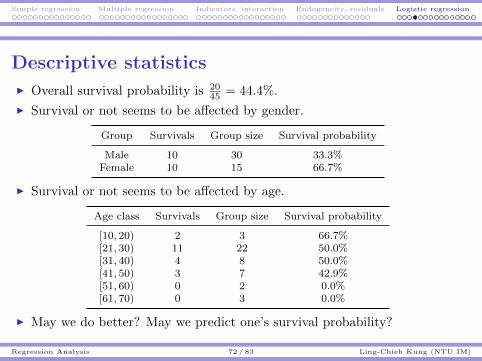
Simple regression Multiple regression Indicators, interaction Endogeneity, residuals Logistic regression
Descriptive statistics
I Overall survival probability is 2045 = 44.4%.
I Survival or not seems to be affected by gender.
Group Survivals Group size Survival probability
Male 10 30 33.3%Female 10 15 66.7%
I Survival or not seems to be affected by age.
Age class Survivals Group size Survival probability
[10, 20) 2 3 66.7%[21, 30) 11 22 50.0%[31, 40) 4 8 50.0%[41, 50) 3 7 42.9%[51, 60) 0 2 0.0%[61, 70) 0 3 0.0%
I May we do better? May we predict one’s survival probability?
Regression Analysis 72 / 83 Ling-Chieh Kung (NTU IM)

Simple regression Multiple regression Indicators, interaction Endogeneity, residuals Logistic regression
Ordinary regression is problematic
I Immediately we may want to construct a linear regression model
survivali = β0 + β1agei + β2femalei + εi.
where age is one’s age, gender is 0 if the person is a male or 1 iffemale, and survival is 1 if the person is survived or 0 if dead.
I By conducting ordinary regression, we may obtain the regression line
survival = 0.746− 0.013age + 0.319female.
Though R2 = 0.1642 is low, both variables are significant.
Regression Analysis 73 / 83 Ling-Chieh Kung (NTU IM)
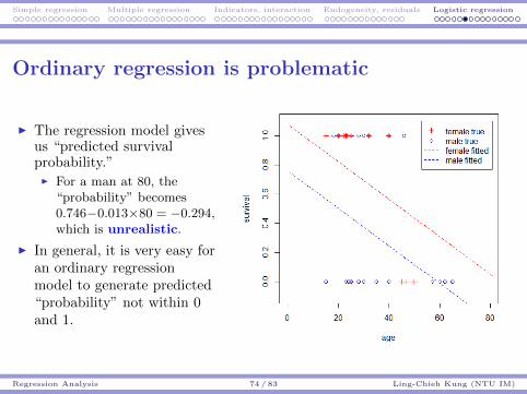
Simple regression Multiple regression Indicators, interaction Endogeneity, residuals Logistic regression
Ordinary regression is problematic
I The regression model givesus “predicted survivalprobability.”I For a man at 80, the
“probability” becomes0.746−0.013×80 = −0.294,which is unrealistic.
I In general, it is very easy foran ordinary regressionmodel to generate predicted“probability” not within 0and 1.
Regression Analysis 74 / 83 Ling-Chieh Kung (NTU IM)

Simple regression Multiple regression Indicators, interaction Endogeneity, residuals Logistic regression
Logistic regression
I The right way to do is to do logistic regression.
I Consider the age-survival example.I We still believe that the smaller age increases the survival probability.I However, not in a linear way.I It should be that when one is young enough, being younger does not
help too much.I The marginal benefit of being younger should be decreasing.I The marginal loss of being older should also be decreasing.
I One particular functional form that exhibits thisproperty is
y =ex
1 + ex⇔ log
(y
1− y
)= x
I x can be anything in (−∞,∞).I y is limited in [0, 1].
Regression Analysis 75 / 83 Ling-Chieh Kung (NTU IM)
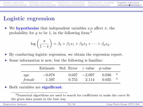
Simple regression Multiple regression Indicators, interaction Endogeneity, residuals Logistic regression
Logistic regression
I We hypothesize that independent variables xis affect π, theprobability for y to be 1, in the following form:3
log
(π
1− π
)= β0 + β1x1 + β2x2 + · · ·+ βpxp.
I By conducting logistic regression, we obtain the regression report.
I Some information is new, but the following is familiar:
Estimate Std. Error z value p-value
age −0.078 0.037 −2.097 0.036 *female 1.597 0.755 2.114 0.035 *
I Both variables are significant.
3Numerical algorithms are used to search for coefficients to make the curve fitthe given data points in the best way.
Regression Analysis 76 / 83 Ling-Chieh Kung (NTU IM)

Simple regression Multiple regression Indicators, interaction Endogeneity, residuals Logistic regression
The Logistic regression curve
I The estimated curve is
log
(π
1− π
)= 1.633− 0.078age + 1.597female,
or equivalently,
π =exp(1.633− 0.078age + 1.597female)
1 + exp(1.633− 0.078age + 1.597female),
where exp(z) means ez for all z ∈ R.
Regression Analysis 77 / 83 Ling-Chieh Kung (NTU IM)

Simple regression Multiple regression Indicators, interaction Endogeneity, residuals Logistic regression
The Logistic regression curve
I The curves can be used todo prediction.
I For a man at 80, π is
exp(1.633−0.078×80)1+exp(1.633−0.078×80) ,
which is 0.0097.
I For a woman at 60, π is
exp(1.633−0.078×60+1.597)1+exp(1.633−0.078×60+1.597) ,
which is 0.1882.
I π is always in [0, 1]. There isno problem for interpretingπ as a probability.
Regression Analysis 78 / 83 Ling-Chieh Kung (NTU IM)
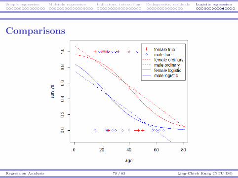
Simple regression Multiple regression Indicators, interaction Endogeneity, residuals Logistic regression
Comparisons
Regression Analysis 79 / 83 Ling-Chieh Kung (NTU IM)

Simple regression Multiple regression Indicators, interaction Endogeneity, residuals Logistic regression
Interpretations
I The estimated curve is
log
(π
1− π
)= 1.633− 0.078age + 1.597female.
Any implication?I −0.078age: Younger people will survive more likely.I 1.597female: Women will survive more likely.
I In general:I Use the p-values to determine the significance of variables.I Use the signs of coefficients to give qualitative implications.I Use the formula to make predictions.
Regression Analysis 80 / 83 Ling-Chieh Kung (NTU IM)
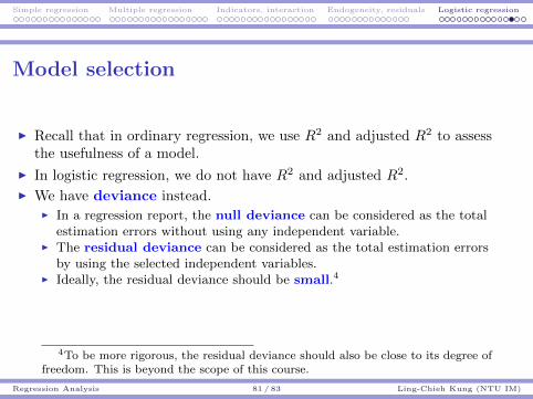
Simple regression Multiple regression Indicators, interaction Endogeneity, residuals Logistic regression
Model selection
I Recall that in ordinary regression, we use R2 and adjusted R2 to assessthe usefulness of a model.
I In logistic regression, we do not have R2 and adjusted R2.
I We have deviance instead.I In a regression report, the null deviance can be considered as the total
estimation errors without using any independent variable.I The residual deviance can be considered as the total estimation errors
by using the selected independent variables.I Ideally, the residual deviance should be small.4
4To be more rigorous, the residual deviance should also be close to its degree offreedom. This is beyond the scope of this course.
Regression Analysis 81 / 83 Ling-Chieh Kung (NTU IM)

Simple regression Multiple regression Indicators, interaction Endogeneity, residuals Logistic regression
Deviances in the regression report
I The null and residual deviances are provided in the regression report.
I For glm(d$survival ~ d$age + d$female, binomial), we have
Null deviance: 61.827 on 44 degrees of freedom
Residual deviance: 51.256 on 42 degrees of freedom
I Let’s try some models:
Independent variable(s) Null deviance Residual deviance
age 61.827 56.291female 61.827 57.286
age, female 61.827 51.256age, female, age× female 61.827 47.346
I Using age only is better than using female only.
I How to compare models with different numbers of variables?
Regression Analysis 82 / 83 Ling-Chieh Kung (NTU IM)
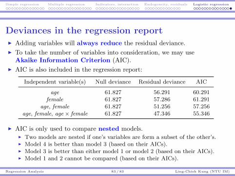
Simple regression Multiple regression Indicators, interaction Endogeneity, residuals Logistic regression
Deviances in the regression reportI Adding variables will always reduce the residual deviance.
I To take the number of variables into consideration, we may useAkaike Information Criterion (AIC).
I AIC is also included in the regression report:
Independent variable(s) Null deviance Residual deviance AIC
age 61.827 56.291 60.291female 61.827 57.286 61.291
age, female 61.827 51.256 57.256age, female, age× female 61.827 47.346 55.346
I AIC is only used to compare nested models.I Two models are nested if one’s variables are form a subset of the other’s.I Model 4 is better than model 3 (based on their AICs).I Model 3 is better than either model 1 or model 2 (based on their AICs).I Model 1 and 2 cannot be compared (based on their AICs).
Regression Analysis 83 / 83 Ling-Chieh Kung (NTU IM)
R for Statistics Public bike rentals
Statistics and Data Analysis for Engineers
Part 4:R for Statistics and Case Studies
Ling-Chieh Kung
Department of Information ManagementNational Taiwan University
September 4, 2016
R for Statistics and Case Studies 1 / 37 Ling-Chieh Kung (NTU IM)

R for Statistics Public bike rentals
Road map
I R for Statistics.
I Public bike rentals.
R for Statistics and Case Studies 2 / 37 Ling-Chieh Kung (NTU IM)
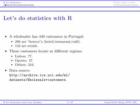
R for Statistics Public bike rentals
Let’s do statistics with R
I A wholesaler has 440 customers in Portugal:I 298 are “horeca”s (hotel/restaurant/cafe).I 142 are retails.
I These customers locate at different regions:I Lisbon: 77.I Oporto: 47.I Others: 316.
I Data source:http://archive.ics.uci.edu/ml/
datasets/Wholesale+customers.
R for Statistics and Case Studies 3 / 37 Ling-Chieh Kung (NTU IM)
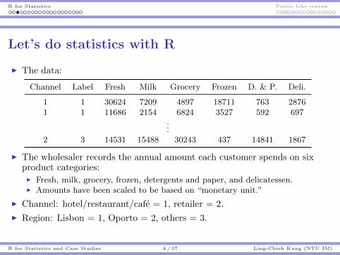
R for Statistics Public bike rentals
Let’s do statistics with R
I The data:
Channel Label Fresh Milk Grocery Frozen D. & P. Deli.
1 1 30624 7209 4897 18711 763 28761 1 11686 2154 6824 3527 592 697
...2 3 14531 15488 30243 437 14841 1867
I The wholesaler records the annual amount each customer spends on sixproduct categories:I Fresh, milk, grocery, frozen, detergents and paper, and delicatessen.I Amounts have been scaled to be based on “monetary unit.”
I Channel: hotel/restaurant/cafe = 1, retailer = 2.
I Region: Lisbon = 1, Oporto = 2, others = 3.
R for Statistics and Case Studies 4 / 37 Ling-Chieh Kung (NTU IM)
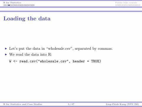
R for Statistics Public bike rentals
Loading the data
I Let’s put the data in “wholesale.csv”, separated by commas.
I We read the data into R:
W <- read.csv("wholesale.csv", header = TRUE)
R for Statistics and Case Studies 5 / 37 Ling-Chieh Kung (NTU IM)

R for Statistics Public bike rentals
Basic statistics
I The mean, median, max, and min expenditure on milk:
mean(W$Milk)
median(W$Milk)
max(W$Milk)
min(W$Milk)
I The sample standard deviation of expenditure on milk:
sd(W$Milk)
I Counting:
length(W[1, ])
length(W[, 1])
R for Statistics and Case Studies 6 / 37 Ling-Chieh Kung (NTU IM)

R for Statistics Public bike rentals
Basic statistics
I Correlation coefficient:
cor(W$Milk, W$Grocery)
I In fact, you may simply do:
W2 <- W[, 3:8]
cor(W2)
I 3:8 is a vector (3, 4, 5, 6, 7, 8).I W[, 3:8] is the third to the eighth columns of W.I cor(W2) is the correlation matrix for pairwise correlation coefficients
among all columns of W2.
R for Statistics and Case Studies 7 / 37 Ling-Chieh Kung (NTU IM)

R for Statistics Public bike rentals
Basic graphs: Scatter plots
plot(W$Grocery, W$Fresh) plot(W$Grocery, W$D Paper)
R for Statistics and Case Studies 8 / 37 Ling-Chieh Kung (NTU IM)

R for Statistics Public bike rentals
Basic graphs: histograms
hist(W$Milk[which(W$Region == 1)])
R for Statistics and Case Studies 9 / 37 Ling-Chieh Kung (NTU IM)

R for Statistics Public bike rentals
Regression with R
I Let’s do regression with R and play with the public bike daily rentaldata set.
I First, let’s load the data:
B <- read.csv("bike day.csv", header = TRUE)
I Take a look at B:
head(B)
mean(B$cnt)
cor(B$cnt, B$temp)
hist(B$cnt)
I Try them!
pairs(B)
pairs(B[, 10:16])
R for Statistics and Case Studies 10 / 37 Ling-Chieh Kung (NTU IM)

R for Statistics Public bike rentals
Simple regression
I Let’s build a simple regression model by using the function lm():
fit <- lm(B$cnt ~ B$instant)summary(fit)
I Put the dependent variable before the ~ operator.I Put the independent variable after the ~ operator.
I We will obtain the regression report:
Coefficients:
Estimate Std. Error t value Pr(>|t|)
(Intercept) 2392.9613 111.6133 21.44 <2e-16 ***
B$instant 5.7688 0.2642 21.84 <2e-16 ***
---
Signif. codes: 0 *** 0.001 ** 0.01 * 0.05 . 0.1 1
Residual standard error: 1507 on 729 degrees of freedom
Multiple R-squared: 0.3954, Adjusted R-squared: 0.3946
F-statistic: 476.8 on 1 and 729 DF, p-value: < 2.2e-16
R for Statistics and Case Studies 11 / 37 Ling-Chieh Kung (NTU IM)

R for Statistics Public bike rentals
Multiple regression
I Let’s add more variables using the + operator:
fit <- lm(B$cnt ~ B$instant + B$workingday + B$temp)summary(fit)
I The regression report:
Coefficients:
Estimate Std. Error t value Pr(>|t|)
(Intercept) -280.3863 138.8325 -2.02 0.0438 *
B$instant 5.0197 0.1925 26.07 <2e-16 ***
B$workingday 145.3731 86.5121 1.68 0.0933 .
B$temp 140.2238 5.4246 25.85 <2e-16 ***
---
Signif. codes: 0 *** 0.001 ** 0.01 * 0.05 . 0.1 1
Residual standard error: 1086 on 727 degrees of freedom
Multiple R-squared: 0.6871, Adjusted R-squared: 0.6858
F-statistic: 532.1 on 3 and 727 DF, p-value: < 2.2e-16
R for Statistics and Case Studies 12 / 37 Ling-Chieh Kung (NTU IM)

R for Statistics Public bike rentals
Interaction
I Let’s consider interaction using the * operator:
fit <- lm(B$cnt ~ B$instant + B$workingday * B$temp)summary(fit)
I The regression report:
Coefficients:
Estimate Std. Error t value Pr(>|t|)
(Intercept) -631.776 204.732 -3.086 0.00211 **
B$instant 5.026 0.192 26.183 < 2e-16 ***
B$workingday 675.120 243.232 2.776 0.00565 **
B$temp 157.912 9.323 16.938 < 2e-16 ***
B$workingday:B$temp -26.471 11.364 -2.329 0.02012 *
---
Signif. codes: 0 *** 0.001 ** 0.01 * 0.05 . 0.1 1
Residual standard error: 1083 on 726 degrees of freedom
Multiple R-squared: 0.6894, Adjusted R-squared: 0.6877
F-statistic: 402.9 on 4 and 726 DF, p-value: < 2.2e-16
R for Statistics and Case Studies 13 / 37 Ling-Chieh Kung (NTU IM)
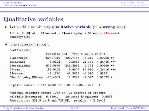
R for Statistics Public bike rentals
Qualitative variablesI Let’s add a non-binary qualitative variable (in a wrong way):
fit <- lm(B$cnt ~ B$instant + B$workingday * B$temp + B$season)summary(fit)
I The regression report:
Coefficients:
Estimate Std. Error t value Pr(>|t|)
(Intercept) -628.7340 208.7156 -3.012 0.00268 **
B$instant 5.0324 0.2085 24.141 < 2e-16 ***
B$workingday 675.0576 243.3996 2.773 0.00569 **
B$temp 158.0409 9.4807 16.670 < 2e-16 ***
B$season -3.1710 41.5623 -0.076 0.93921
B$workingday:B$temp -26.4682 11.3722 -2.327 0.02022 *
---
Signif. codes: 0 *** 0.001 ** 0.01 * 0.05 . 0.1 1
Residual standard error: 1083 on 725 degrees of freedom
Multiple R-squared: 0.6894, Adjusted R-squared: 0.6873
F-statistic: 321.9 on 5 and 725 DF, p-value: < 2.2e-16
R for Statistics and Case Studies 14 / 37 Ling-Chieh Kung (NTU IM)

R for Statistics Public bike rentals
Qualitative variables
I To correctly include a qualitative variable, use the function factor():
fit <- lm(B$cnt ~ B$instant + B$workingday * B$temp + factor(B$season))summary(fit)
I factor() tells the R program to interpret those values as categories evenif they are numbers.
I If the values are already non-numeric, there is no need to use factor().
I Let’s read the regression report.
R for Statistics and Case Studies 15 / 37 Ling-Chieh Kung (NTU IM)

R for Statistics Public bike rentals
Qualitative variables
I The regression report:1
Coefficients:
Estimate Std. Error t value Pr(>|t|)
(Intercept) -749.4834 209.3085 -3.581 0.000366 ***
B$instant 5.1296 0.2015 25.459 < 2e-16 ***
B$workingday 632.4411 233.8650 2.704 0.007006 **
B$temp 146.5942 11.7999 12.423 < 2e-16 ***
factor(B$season)2 827.2798 143.1463 5.779 1.12e-08 ***
factor(B$season)3 142.7658 188.6595 0.757 0.449454
factor(B$season)4 272.6144 126.7112 2.151 0.031770 *
B$workingday:B$temp -24.5086 10.9264 -2.243 0.025195 *
---
Signif. codes: 0 *** 0.001 ** 0.01 * 0.05 . 0.1 1
Residual standard error: 1041 on 723 degrees of freedom
Multiple R-squared: 0.7142, Adjusted R-squared: 0.7115
F-statistic: 258.2 on 7 and 723 DF, p-value: < 2.2e-16
1To change the reference level, use relevel().
R for Statistics and Case Studies 16 / 37 Ling-Chieh Kung (NTU IM)

R for Statistics Public bike rentals
Variable transformation
I To add temp2:
tempSq <- B$temp^2
fit <- lm(B$cnt ~ B$instant + B$workingday * (B$temp + tempSq))summary(fit)
I The regression report:
Coefficients:
Estimate Std. Error t value Pr(>|t|)
(Intercept) -3313.2904 462.5027 -7.164 1.93e-12 ***
B$instant 4.7928 0.1874 25.576 < 2e-16 ***
B$workingday 1934.5264 578.2195 3.346 0.000863 ***
B$temp 482.5310 50.6541 9.526 < 2e-16 ***
tempSq -8.1197 1.2489 -6.501 1.48e-10 ***
B$workingday:B$temp -180.0186 62.5810 -2.877 0.004138 **
B$workingday:tempSq 3.9116 1.5382 2.543 0.011200 *
---
Signif. codes: 0 *** 0.001 ** 0.01 * 0.05 . 0.1 1
R for Statistics and Case Studies 17 / 37 Ling-Chieh Kung (NTU IM)
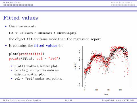
R for Statistics Public bike rentals
Fitted values
I Once we execute
fit <- lm(B$cnt ~ B$instant + B$workingday)
the object fit contains more than the regression report.
I It contains the fitted values yi:
plot(predict(fit))
points(B$cnt, col = "red")
I plot() makes a scatter plot.I points() add points onto an
existing scatter plot.I col = "red" makes red points.
R for Statistics and Case Studies 18 / 37 Ling-Chieh Kung (NTU IM)
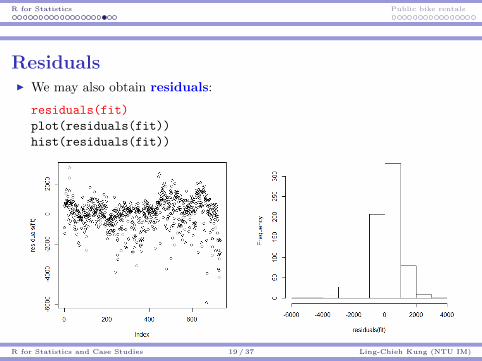
R for Statistics Public bike rentals
ResidualsI We may also obtain residuals:
residuals(fit)
plot(residuals(fit))
hist(residuals(fit))
R for Statistics and Case Studies 19 / 37 Ling-Chieh Kung (NTU IM)

R for Statistics Public bike rentals
Logistic regression in R
I To run logistic regression in R, all we need to do is to:I Replace lm() by glm().I Add a new parameter binomial.
I Let’s load the survival data set:
d <- read.csv("survival.csv", header = TRUE)
R for Statistics and Case Studies 20 / 37 Ling-Chieh Kung (NTU IM)
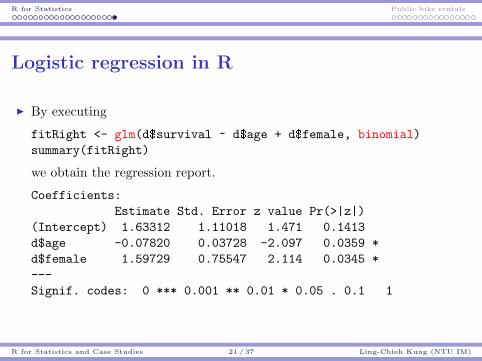
R for Statistics Public bike rentals
Logistic regression in R
I By executing
fitRight <- glm(d$survival ~ d$age + d$female, binomial)
summary(fitRight)
we obtain the regression report.
Coefficients:
Estimate Std. Error z value Pr(>|z|)
(Intercept) 1.63312 1.11018 1.471 0.1413
d$age -0.07820 0.03728 -2.097 0.0359 *
d$female 1.59729 0.75547 2.114 0.0345 *
---
Signif. codes: 0 *** 0.001 ** 0.01 * 0.05 . 0.1 1
R for Statistics and Case Studies 21 / 37 Ling-Chieh Kung (NTU IM)

R for Statistics Public bike rentals
Road map
I R for Statistics.
I Public bike rentals.
R for Statistics and Case Studies 22 / 37 Ling-Chieh Kung (NTU IM)

R for Statistics Public bike rentals
Public bike rental data set
I Recall our daily bike rental data set (in “bike day.csv”).I For each day in 2011 and 2012, we have the number of rentals of public
bikes in Washington, D.C.I There are 731 rows representing the 731 days in the time horizon.
I Data source: http://archive.ics.uci.edu/ml/datasets/Bike+Sharing+Dataset.
I There are sixteen columns as explained below.
R for Statistics and Case Studies 23 / 37 Ling-Chieh Kung (NTU IM)

R for Statistics Public bike rentals
The sixteen variables
I (Serial number) instant : A serial number from 1 to 731.
I (Date information) date, year, season, month: the labels of that date.
I (Working information) holiday, weekday, workingday :I holiday is 1 if that day is a national holiday not in a weekend and 0
otherwise;I weekday labels whether it is Sunday (labeled as 0), Monday (labeled as
1), ..., or Saturday (labeled as 6);I workingday is 1 if that day is a working day (neither a weekend nor a
holiday) and 0 otherwise.
R for Statistics and Case Studies 24 / 37 Ling-Chieh Kung (NTU IM)

R for Statistics Public bike rentals
The sixteen variables
I (Weather information) Five attributes are recorded in this category:I weathersit (weather situation): 1 for sunny or partly cloudy, 2 for misty
and cloudy, 3 for light snow or light rain, and 4 for heavy snow orthunderstorm.
I temp (temperature) and atemp (apparent temperature): the dailyaverage of temperature and apparent temperature (in Celsius),respectively.
I humidity : the daily average of the humidity (in %).I windspeed (wind speed): the daily average of the wind speed (in knot; 1
knot is around 1.852 km/h).
I (Rental data) casual, registered, cnt :I casual is the number of rentals made by unregistered users.I registered is the number of rentals made by registered members.I cnt is the sum of the two numbers.
R for Statistics and Case Studies 25 / 37 Ling-Chieh Kung (NTU IM)

R for Statistics Public bike rentals
Questions
I What are the relationships among these variables?
I How do these variables affect the rental outcomes?
I How to build a model to explain the variability of rental outcomes?
I How to build a model to predict future rental outcomes?
R for Statistics and Case Studies 26 / 37 Ling-Chieh Kung (NTU IM)
R for Statistics Public bike rentals
Descriptive Statistics
I What are the summaries of these variables?
I What are the shapes of distributions of these variables?
I Are there correlation among these variables?
R for Statistics and Case Studies 27 / 37 Ling-Chieh Kung (NTU IM)
R for Statistics Public bike rentals
Capturing the trend
I Construct a regression model for instant and cnt. Do you still see anincreasing trend?
R for Statistics and Case Studies 28 / 37 Ling-Chieh Kung (NTU IM)

R for Statistics Public bike rentals
Impact of working/holiday
I Construct a regression model for instant and cnt. Do you still see anincreasing trend?
I Add the variable holiday into the regression model. In average what isthe impact of being a holiday?
I Remove holiday and add the column workingday into the regressionmodel. In average what is the impact of being a working day?Compare the result with holiday.
R for Statistics and Case Studies 29 / 37 Ling-Chieh Kung (NTU IM)

R for Statistics Public bike rentals
Impact of weather (quantitative variables)
I How do temp, atemp, hum, and windspeed affect cnt?
I If you used a regression model with the five variables listed in (a),what are the potential drawbacks?
I Try to take away temp and do the analysis again.
I Try to add instant and do the analysis again.
R for Statistics and Case Studies 30 / 37 Ling-Chieh Kung (NTU IM)
R for Statistics Public bike rentals
Impact of weather (transformation)
I Some people suggest that temp should have a nonlinear impact on cnt.Does this fit your intuition? Draw a scatter plot to help you judge theintuition.
I To capture the nonlinear relationship, let’s add a variable temp2 as oursecond independent variable. Construct the regression model, interpretit, and validate it.
I Does adding temp2 improves the model?
I Visualize the two regression models.
R for Statistics and Case Studies 31 / 37 Ling-Chieh Kung (NTU IM)
R for Statistics Public bike rentals
Impact of weather (qualitative variables)
I If we construct a regression model with instant, weathersit, and cnt,what is wrong?
I Create indicator variables for weathersit by choosing sunny as thereference level. Construct a regression model with instant, the indicatorvariables for weathersit, and cnt. Validate and interpret the model.
R for Statistics and Case Studies 32 / 37 Ling-Chieh Kung (NTU IM)
R for Statistics Public bike rentals
Seasonality
I Use instant, season, and cnt to build a model.
I What if we replace season by month?
R for Statistics and Case Studies 33 / 37 Ling-Chieh Kung (NTU IM)
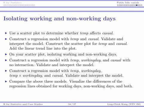
R for Statistics Public bike rentals
Isolating working and non-working days
I Use a scatter plot to determine whether temp affects casual.
I Construct a regression model with temp and casual. Validate andinterpret the model. Construct the scatter plot for temp and casual.Add the linear trend line into the plot.
I On your scatter plot, isolating working and non-working days.
I Construct a regression model with temp, workingday, and casual withno interaction. Validate and interpret the model.
I Construct a regression model with temp, workingday,temp× workingday, and casual. Validate and interpret the model.
I Compare the above three models. Visualize the differences of theregression lines obtained for working days, non-working days, and both.
R for Statistics and Case Studies 34 / 37 Ling-Chieh Kung (NTU IM)

R for Statistics Public bike rentals
Isolating working and non-working days
I Construct a multiple linear regression model with temp, workingday,temp× workingday, and cnt. Validate and interpret the model.
I Visualize the differences of the regression lines obtained for workingdays, non-working days, and both.
R for Statistics and Case Studies 35 / 37 Ling-Chieh Kung (NTU IM)

R for Statistics Public bike rentals
Using casual and registered
I To predict or explain cnt, is it good to include casual or registered asindependent variables?
R for Statistics and Case Studies 36 / 37 Ling-Chieh Kung (NTU IM)
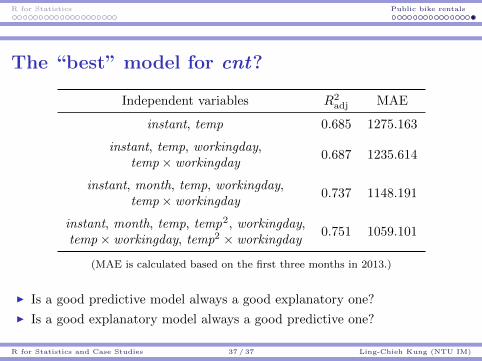
R for Statistics Public bike rentals
The “best” model for cnt?
Independent variables R2adj MAE
instant, temp 0.685 1275.163
instant, temp, workingday,0.687 1235.614
temp× workingday
instant, month, temp, workingday,0.737 1148.191
temp× workingday
instant, month, temp, temp2, workingday,0.751 1059.101
temp× workingday, temp2 × workingday
(MAE is calculated based on the first three months in 2013.)
I Is a good predictive model always a good explanatory one?
I Is a good explanatory model always a good predictive one?
R for Statistics and Case Studies 37 / 37 Ling-Chieh Kung (NTU IM)